Sage Journals: Discover world-class research

Abstract

The titanium alloy open integral micro impeller has a strong material strength and high removal rate in the field of multi-axis CNC machining. The flow channel is tiny and the blades are thin and highly twisted. It is difficult to control the surface accuracy and prone to overcutting and undercutting. The NX2212 software post-processing module plans two distinct blade finishing process routes and verifies them using virtual machine tool simulation, taking into account the technical challenges of micro impeller machining. Following verification, the tool path machining code is imported into MATLAB for data fitting. The workpiece surface working condition is determined based on the simulation findings, the blade surface roughness value is calculated, and a physical simulation model of blade finishing is created in the finite element analysis software. The outcomes demonstrate how well the “segmented and sub-regional cutting” processing method may raise blade accuracy. The leading and trailing edges of the blade both had surface roughness increases of 4.86% and 4.19%. The surface morphology of the micro impeller is measured using a white light interferometer, and it is CNC machined using two distinct process methods. The findings demonstrate that there is a significant difference between the value calculated by the finite element analysis software and the surface roughness value measured experimentally which together make up less than 5%. An investigation of the impact of cutting parameters on the surface roughness of micro-structure components is carried out using a three factor, three-level BBD experiment that is founded on the second-order response surface method. The findings indicate that the feed per tooth influences surface roughness more significantly than cutting depth and cutting speed for a reasonable range of cutting parameters; Surface roughness will rise with lower or higher cutting speeds; Raising the feed per tooth and the cutting speed simultaneously may reduce surface roughness; Surface roughness can be accurately predicted and controlled using the second-order response surface method.

Keywords

Integral micro impeller tool path finite element analysis surface roughness response surface method

Introduction

An essential component of the national economy, the advanced manufacturing sector is a key pillar for maintaining national security and serves as a gauge for nation’s or region’s overall strength as well as its degree of science and technology.¹ The development of advanced manufacturing industry is one of the important strategic measures to improve China’s own comprehensive strength and learn from developed countries in Europe and America.² During the “11th Five-Year Plan,”“12th Five-Year Plan,”“13th Five-Year Plan,” and at the beginning of the “14th Five-Year Plan,” China has formulated a number of major R&D plans such as “Made in China 2025,”“13th Five-Year Plan National Science and Technology Innovation Plan,”“Mechanical Engineering Discipline Development Strategy Report 2011–2020,” and “2035 Standard Plan.” The goal is to realize the grand strategy of building our country from a big manufacturing country into a powerful manufacturing country.³ It has greatly promoted the high-quality development of my country’s politics, economy, culture, society, and ecology.⁴

The only metals with higher earthly abundance are titanium, followed by iron (Fe), aluminum (Al), and magnesium (Mg). High specific strength, strong thermal strength, low temperature performance, and superior corrosion resistance are among the properties of titanium and titanium alloy.⁵ Because of these benefits, nations all over the world have intensified their efforts to prepare new titanium alloy as well as their research and use of titanium alloy in the field of sophisticated manufacturing since the 1950s.⁶ Based on their annealed structures, titanium alloy at room temperature can be broadly classified into three groups: α titanium alloy, β titanium alloy, and α + β titanium alloy. TC is the brand name for α + β titanium alloy, which is also known as two-phase titanium alloy.⁷ This material exhibits exceptional strength at high temperatures and outstanding resistance to oxidation, combining the benefits of α and β titanium alloy.⁸ Because of their superior qualities, titanium alloy materials are frequently employed in high-temperature, high-pressure, and high-wear extremes – that is, in precision-critical elements like engine support shafts, aeroengine transmission casings, and impeller blades.⁹ However, titanium alloy is a challenging material with low thermal conductivity, low elastic modulus, high friction coefficient, low hardness, and high chemical activity. As a result, the tool tip absorbs the majority of the heat generated during cutting in an environment with high pressure and temperature. The hardening layer that forms on the workpiece surface will have an impact on cutting stability, and material rebound on the workpiece surface in the third deformation zone will increase wear on the back tool surface.¹⁰ The open integral micro impeller is an important component in the marine, chemical, and environmental protection industries. It is extensively employed in flow measurement, air purification, and transportation and mixing of different liquids due to its strong self-priming ability and outstanding performance in handling high-viscosity media.¹¹ It is a typical thin-walled part, which is mainly composed of non-developable ruled surfaces and spatially curved surfaces; the shape of the impeller blades is rotated and twisted, and the radius curvature of the leading and trailing edges of the blades changes greatly. Because of the small space between neighboring blades, it is necessary to cut the blade surface, root, flow channel surface, and other components in layers over the course of several processes.¹² Processing challenges arise since the open integral micro impeller’s primary materials are titanium alloy and other hard-to-machine materials.¹³

Currently, the mechanical field uses a variety of open integral impeller engineering processes, and operators frequently employ CNC milling, electrolytic machining, casting, EDM, and other techniques.¹⁴ However, multi-axis CNC machining of open integral impellers has drawn a lot of interest in the industry due to the quick development of advanced manufacturing and precise machine tool automation.¹⁵ Liang and Wang¹⁶ studied the roughing of the hub surface of the titanium alloy integral impeller. The quaternion interpolation technique was creatively used to control the tool axis vector, and the roughing cutting path of the hub surface was developed and experimentally tested in order to ensure a high material removal rate and processing efficiency. It was determined that the algorithm could significantly raise the impeller roughing’s overall cutting efficiency. Li et al.¹⁷ investigated the suction surface finishing of a titanium alloy integral impeller and creatively processed the suction surface using nonuniform rational B-spline interpolation. After planning and experimentally verifying the tool axis vector in an open computer numerical control system, it was determined that the interpolation technique could produce smooth and continuous motion of the motion axis. Stratogiannis et al.¹⁸ studied the finishing of aluminum alloy semi-closed radial impeller blade, used professional CAM software NX to plan the best cutting parameters and tool parameters of the blade finishing process, through orthogonal experiments, the cutting process was verified, and it was found that the optimal cutting parameters were determined. Additionally, the spindle speed and feed per tooth had a significant impact on the cutting performance. Han et al.¹⁹ studied the finishing machining of high-temperature alloy integral impeller flow channels. Creatively optimized the tool parameters by using the minimum processing time as the objective function and the depth priority approach to choose tool parameters judiciously in various cutting layers. Comparative experiments demonstrate that the approach can increase cutting efficiency. Li et al.²⁰ studied the finishing of titanium alloy integral impeller blades. Coupled multi-objective parameter optimization with digital twin technology in an inventive way, computed the chip area and milling force with precision using numerical simulation techniques, and validated the model using comparative trials. About 8% more precision may be obtained with the optimized milling force prediction model. Soori and Asmael²¹ conducted research on the finishing of titanium alloy integral impeller flow channels. A novel virtual machining system was created to optimize the milling path based on numerical simulation and genetic algorithms in order to prevent the overcutting phenomenon of five-axis CNC machine tools during the machining process. The feasibility of the milling path was confirmed through experiments, and the processed impeller was measured using a three-dimensional coordinate measuring machine. It was determined that the system can increase processing accuracy and efficiency. Feng et al.²² conducted research on the finishing of aluminum alloy integral impeller root fillet. The novel approach uses cognitive processing to online monitor the burr shape of the blade root and adjust the cutter axis vectors and cutting settings to prevent over-cutting of the five-axis CNC machine tool during processing.

One of the key metrics for assessing the quality of the machining process throughout the cutting process is the machined surface roughness, which is the outcome of the combined influence of various elements including the condition of the equipment, the cutting parameters, and the tool structure.²³ At the moment, an offline approach of measuring the workpiece’s surface roughness is widely used. However, complicated parts’ offline surface roughness has a low efficiency and high detection cost, which significantly increases the cost of component processing and manufacturing cycles.²⁴ Accurately predicting machined surface roughness during the milling of intricate, specially-shaped objects has garnered a lot of interest from academics.²⁵ Yang et al.²⁶ used orthogonal experiments to study the effects of tool inclination and micro texture parameters on the machining surface quality during titanium alloy milling. A surface roughness prediction model that took into account the micro-texture characteristics and tool inclination was developed using the multiple linear regression analysis method, and the multiple linear regression equation’s relevance was confirmed. Savas et al.²⁷ investigated the effects of tool settings, cutting parameters, and working condition stability on the workpiece’s surface roughness during the combined machining of 100Cr6 steel by using a single factor experiment approach. The results identified the ideal cutting parameters for the combined machining of 100Cr6 steel and demonstrated that the spindle speed had a significant impact on surface roughness. Zhang et al.²⁸ studied the influence of laser shot peening process parameters on the surface roughness and hardness of aerospace critical parts for structural repair. The optimal laser shot peening process parameters were found based on the experimental findings, which demonstrated that the workpiece’s surface roughness decreased and its hardness increased following laser shot peening treatment. Lin et al.²⁹ studied the influence of milling parameters and vibration on surface roughness during milling of Al6061 aluminum alloy, The study also compared the predictive power of neural network and multiple regression analysis models on surface roughness, with the neural network model predicting surface roughness better than the multiple regression analysis model. Li et al.³⁰ optimized the least squares support vector machine based on the particle swarm algorithm, taking the feature value of noise, vibration, and the surface texture of the workpiece as the input value, and the roughness as the output value to build a Ra prediction model of multi-dimensional feature fusion. This model achieves a prediction accuracy of 92.54%. Nouhi and Pour³¹ used a non-contact approach to assess the online surface roughness, combined the wavelet method with two-dimensional surface photography to extract the surface texture. By extracting the surface texture’s time delay parameters, which were able to forecast the texture’s trend and make adjustments to the processing parameters. This technology offers a fresh approach to surface roughness prediction and can be applied to grinding, turning, and milling operations. Deng et al.³² also used online surface roughness measurement. The surface roughness prediction model under the fixed work-tool combination was constructed by using electrical signals output from time and frequency domain features, such as force, acceleration, and temperature sensors. The accuracy and stability of the entire system under working conditions were confirmed on the machining center.

Based on the study mentioned above, this article first establishes a three-dimensional model of an open integral micro impeller in the CAM software NX2212 modeling module. Two processing routes are employed to finish the blades in the processing module, which also roughens the flow channel and integrally roughens the blank. Verifying the rationality and safety of the two finishing routes in the virtual machine tool simulation module, exporting the G code in the post-processing module and fitting the data through MATLAB software. Secondly, the tool and workpiece are positioned and loaded in the STL format into the finite element analysis program DEFORM-3D in the assembly module. The DEFORM-3D pre-processing module sets the variables for the simulation environment, while the post-processing module obtains the necessary physics field curves. The surface roughness value of each area is calculated theoretically, the two early-stage planned finishing routes are mounted on the machine, and the surface topography of the micro impeller entity is measured using a white light interferometer. Finally, a three-factor, three-level BBD experiment based on the second-order response surface approach is constructed in order to further increase the forecast accuracy of the surface roughness of micro-structural parts. The significance analysis of the experimental results is carried out, and a response surface diagram of surface roughness and cutting parameters is created. Experiments confirms the prediction model’s accuracy.

Multi-axis CNC finishing process of open integral micro impeller

The tiny blade thickness, restricted flow route, and severe blade distortion of the titanium alloy open integral micro impeller make it an essential part of aeronautical micro engines. Large material removal rates during machining can easily result in overcutting or tool interference; also, standard three and four axis machine tools have trouble maintaining surface accuracy and processing quality.³³ With their intersecting spindles, five axis CNC machine tools offer significant advantages when processing curved surfaces that are spatially complicated.³⁴ In order to address the issues of overcutting, undercutting, and interference during the CNC machining of the open impeller, a suitable machining process route, tool kinds, and tool parameters are developed by examining the structural features of the open impeller (Figure 1) depicts the open impeller’s structure.

Figure 1.

The structure of the open impeller: (a) top view, (b) main view, and (c) side view.

Finishing process of open integral micro impeller

The influence of several processing paths on the final blade’s surface accuracy and machining quality is the main topic of this article. The goal of blade finishing is to increase surface accuracy, which enhances the blade’s operational efficiency. It is also one of the key indicators that guarantee the impeller runs steadily.

Opening the NX2212 software and entering the processing module, creating the blank geometry, setting the processing process route, tool parameters, cutting parameters to rough the flow channel. Larger feed speeds are typically employed during the roughing process in order to expeditiously remove blank extra material, which is advantageous for finishing that follows. The Figure 2 displays the tool path that the runner roughing produced. The semi-finishing runner’s tool path and roughing match those of the finishing runner.

Figure 2.

Roughing process: (a) blank geometry, (b) process routes and tool parameters, and (c) rough the flow channel.

Side blade milling is the cutting technique used to complete the blade. The working parameters such as workpiece stiffness and tool attitude fluctuate during cutting because of the variations in the curvature of the blade’s individual parts as well as the differences in thickness of the blade’s root and edge. Two distinct machining paths were chosen for finishing in order to investigate the effects of these methods on the precision and quality of the machining of the blade surface. The first finishing machining route and tool parameters are shown in the Figure 3, the tool axis is adjusted to be processed by the smooth interpolation vector. Typically, this technique is referred to as the “one-tool flow” machining process. One benefit of it is that it can lessen to a certain extent, processing efficiency can be increased by the tool’s idle time during cutting. Because the leading and trailing edges of the blade have varying thicknesses, undercutting could result from processing the blade using smooth interpolation in variable profile milling, which would prevent the blade accuracy from meeting specifications. Therefore, a second finishing route is proposed, as shown in the Figures 4 and 5. In fixed contour milling, the tool axis is controlled to process the designated plane normal direction for the blade leading edge and trailing edge area. In variable contour milling, the tool axis is still regulated to be processed using the smooth interpolation vector for the blade suction surface and pressure surface area. The “segmented and sub-regional cutting” processing method is the name given to this technique, which employs various cutting techniques for various morphological aspects. Its benefit is that it will somewhat increase the blade’s leading and trailing edge accuracy; nevertheless, overall cutting efficiency will be marginally decreased.

Figure 3.

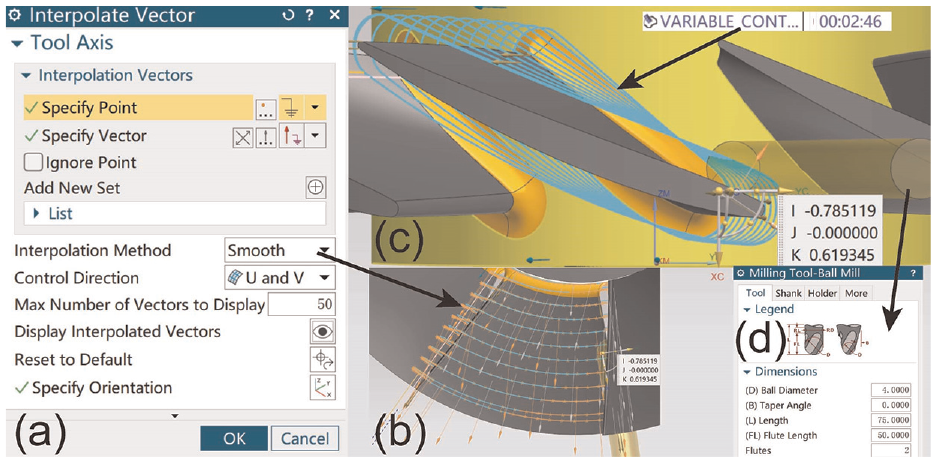
First processing: (a) interpolate vector, (b) the smooth interpolation vector, (c) tool path, and (d) tool paraments.

Figure 4.

The method of blade leading edge and trailing edge: (a) fix contour milling and (b) tool path.

Figure 5.

The method of blade suction and pressure surface area: (a) interpolate vector and (b) tool path.

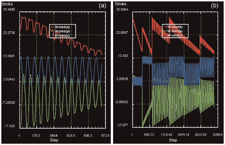
The tool path is verified using the virtual machine tool included with the NX2212 software post-processing module in order to confirm the precision and logic of the machining route. To align the machine tool coordinate system with the workpiece coordinate system, switch to the machine tool view interface, choose the Fanuc system A-C double swing head five-axis vertical machining center, and utilize component installation connections. The workpiece and established machine tool are depicted in the Figure 6(a). Overcut and collision inspections are carried out, and the two finishing routes are simulated respectively. The actual tool path is as shown in the Figure 6(b) to (d). Once processing is finished, it can be determined by looking at the tool path to make sure there isn’t any overcutting or collision phenomena when cutting, meaning that both processing paths can finish the blade. Following verification of the tool path, the data is processed into a point set, fitted using MATLAB, and the G code of the CNC program is exported in the NX2212 software post-processing module. The Figure 7 displays the two finishing routes as well as the MATLAB software. When looking at the machining path in the Figure 7(b) and (c), it is clear that the tool path created by variable profile milling on the leading and trailing edge areas of the blade is less dense than the tool path created by fixed profile milling on those same areas.

Figure 6.

NX2212 software post-processing module: (a) machine tool and workpiece, (b) first tool path, (c) second tool path, and (d) second tool path.

Figure 7.

Fitted using MATLAB: (a) MATLAB software, (b) first finishing routes, and (c) second finishing routes.

Surface roughness acquisition and experimental verification based on finite element analysis

The implementation of digital twin technology, or the interactive mapping of digital models built in virtual space and physical entities, has gradually become possible thanks to the development of new generation information technologies like the Internet of things, Big Data, Cloud Computing, and Artificial Intelligence.³⁵ This allows for an accurate description of the operation trajectory of a physical entity’s entire life cycle.³⁶ Digital twins are seen as an efficient way to achieve the interactive integration of the industrial information world and the physical world, particularly in the field of intelligent manufacturing.³⁷ The open integral micro impeller’s multi-axis CNC finishing path has been identified previously. To investigate the impact of two distinct finishing pathways and varying cutting parameters on blade surface roughness, a multi-physical field coupling model was developed for blade finishing, and numerical simulation was conducted from a mathematical model construction standpoint.

Utilizing sophisticated mathematical theory and potent adaptive meshing technology, SFTC’s DEFORM-3D software has been extensively employed in rolling, rolling, metal plastic forming, and cutting operations. A great deal of microscopic information that is difficult to collect directly through tests can be gathered with the aid of DEFORM-3D software.³⁸ Mali et al.³⁹ performed a finite element analysis of the dry cutting of 7075 aluminum alloy using the finite element modeling program DEFORM-3D. To ascertain the impact of cutting elements on cutting forces, the study employed multiple linear regression analysis and variance analysis. Cutting experiments were used to confirm the correctness of the simulation results, and by predicting the cutting force, the number of cutting trials required was significantly decreased. Maity and Pradhan⁴⁰ used SolidWorks software to create a micro-groove cutting insert model, imported the model into DEFORM-3D software and conducted a finite element analysis of the titanium alloy cutting process. Cutting temperature, effective stress, and tool wear rate simulation cloud diagrams were created in the post-processing module, and certain simulation results were confirmed by cutting experiments. In order to optimize the tool model, the simulation findings and the experimental results agreed rather well.

Establishment of finite element simulation model based on DEFORM-3D

A ball-end milling cutter model with consistent tool parameters and Figure 3(d) is built in the NX2212 software modeling module because ball-end milling cutters are frequently used for processing complex surfaces and have strong cutting processing adaptability. The tool handle is shortened to decrease the amount of successive tool mesh divisions and speed up the simulation. In order to reflect the finishing process of titanium alloy open integral micro impeller blades more accurately, the ball-end milling cutter and micro impeller are assembled in NX2212 software, and the tool feeding process is omitted at the assembly position. Based on the previously exported point set map and G code. The cutting positions of the first finishing route tool are determined to be: X: 25.911, Y: −16.842, Z: 10.808, as shown in the Figure 8(a). The second finishing route tool is: X: 30.4, Y: 5.637, Z: 6.305, as shown in the Figure 8(b). The tool and micro impeller maintained their relative position relationship when they were saved as STL format files and integrated into the DEFORM-3D environment. The workpiece and the tool are meshed to better represent the cutting process. The number of meshes is 150,000 and 50,000 respectively. The meshing results are shown in the Figure 9.

Figure 8.

Assembly module: (a) first finishing routes and (b) second finishing routes.

Figure 9.

Simulation module: (a) first finishing routes and (b) second finishing routes.

Large deformation, high strain rates, and complicated elastic-plastic deformation are all part of the metal cutting process, which produces a lot of cutting force and intense heat. In order to specify the workpiece and tool materials, the Johnson-Cook constitutive model which is more suited for metal cutting is chosen.⁴¹ The Johnson-Cook constitutive model is composed of three components: the temperature effect associated with flow stress, the strain hardening effect, and the strain rate effect. As indicated by the following equation (1).

\bar{σ} = (A + B ε^{n}) (1 + Cln \frac{\overset{\cdot}{ε}}{ε_{0}}) [1 - {(\frac{T - T_{amb}}{T_{melt} - T_{amb}})}^{m}]

(1)

In the equation (1), A, B, n, C, and m are material property strengthening term constants; T_melt is the melting point; T_amb is room temperature; ε is the reference strain rate. Check the literature⁴² the Johnson-Cook constitutive model of TC11 is:

\begin{matrix} \bar{σ} = (1309 + 258 ε^{0.44}) (1 + 0.0047 \ln \frac{\overset{\cdot}{ε}}{ε_{0}}) \\ [1 - {(\frac{T - T_{amb}}{T_{melt} - T_{amb}})}^{0.99}] \end{matrix}

(2)

In the DEFORM-3D material library, select the workpiece material as TC11, the grade as TI-6Al-6V-2Sn, and the tool material as WC carbide. The workpiece type is selected as a plastic body. To consider the problem of tool wear during processing, the tool type is selected as an elastic-plastic body. Imposing preset limitations on the workpiece’s XYZ direction and programming the tool to follow a predetermined path. The tool itself revolves clockwise around the fixed Z axis, as seen in the Figure 10. The rotation speed is set to n = 8000 r/min, which is converted to ω = 837.757 rad/s. The initial temperature of the simulated environment was adjusted to 20°C, the friction coefficient was set to 0.6, the thermal conductivity coefficient to 45 m² s K, and the heat transfer coefficient to 0.02 after examining pertinent literature⁴³ and combining experience and common sense. As indicated in the Figure 11(a), selected the “Usui” kind of wear formula and based on prior experience choosing coefficients under the wear conditions, a = 0.0000001, b = 855. As indicated in the Figure 11(b), selected the incremental simulation option and ensured that the storing is done every 50 steps and the new settings are executed every 100,000 steps.

Figure 10.

Tool path: (a) first finishing routes and (b) second finishing routes.

Figure 11.

Simulation parameter settings: (a) “Usui” wear model and (b) step count settings.

Verifying the pertinent setup options after finishing the pre-processing of the micro impeller’s finite element simulation. The.DB file needed for the simulation computation can be created if the check is corrected. Next, going back to the DEFORM-3D main interface, choosing the.DB file that requires calculation, and carrying out finite element simulation using the pre-processing module’s specified number of simulation steps until the step count is determined. Lastly, the post-processing module allows users to evaluate simulation outcomes like cutting force and temperature during the cutting process. The cutting force and temperature curves for two distinct finishing approaches are displayed in the Figures 12 and 13 as they change over time. The X, Y, and Z cutting forces in the Figure 12(a) to (c) increase gradually, exhibit periodic variations without noticeably abrupt changes, and progressively tend to be stable, suggesting the plausibility of the micro impeller cutting force finite element modeling technique; The growth rate gradually decreases as the cutting temperature in the Figure 12(d) rises from the ambient temperature of 20°C. There are no obvious multiple abrupt changes throughout the entire machining process, and it gradually tends to be stable, suggesting that the finite element simulation process of the micro impeller’s cutting temperature is credible. The abrupt change phenomenon at the marks in the Figure 12(d) may be caused by the abrupt rise in temperature brought on by mesh distortion. Likewise, the Figure 13 is cutting force and temperature curves with time can also depict the second finishing route’s operation more precisely. When the abrupt changes in the figure are taken out of account, comparative computation and analysis reveal that the first finishing route’s XYZ three directions have lower average cutting force, peak cutting force, average cutting temperature, and peak cutting temperature than the second finishing route. Thus, the first finishing path is preferable in terms of total power consumption during cutting procedure.

Figure 12.

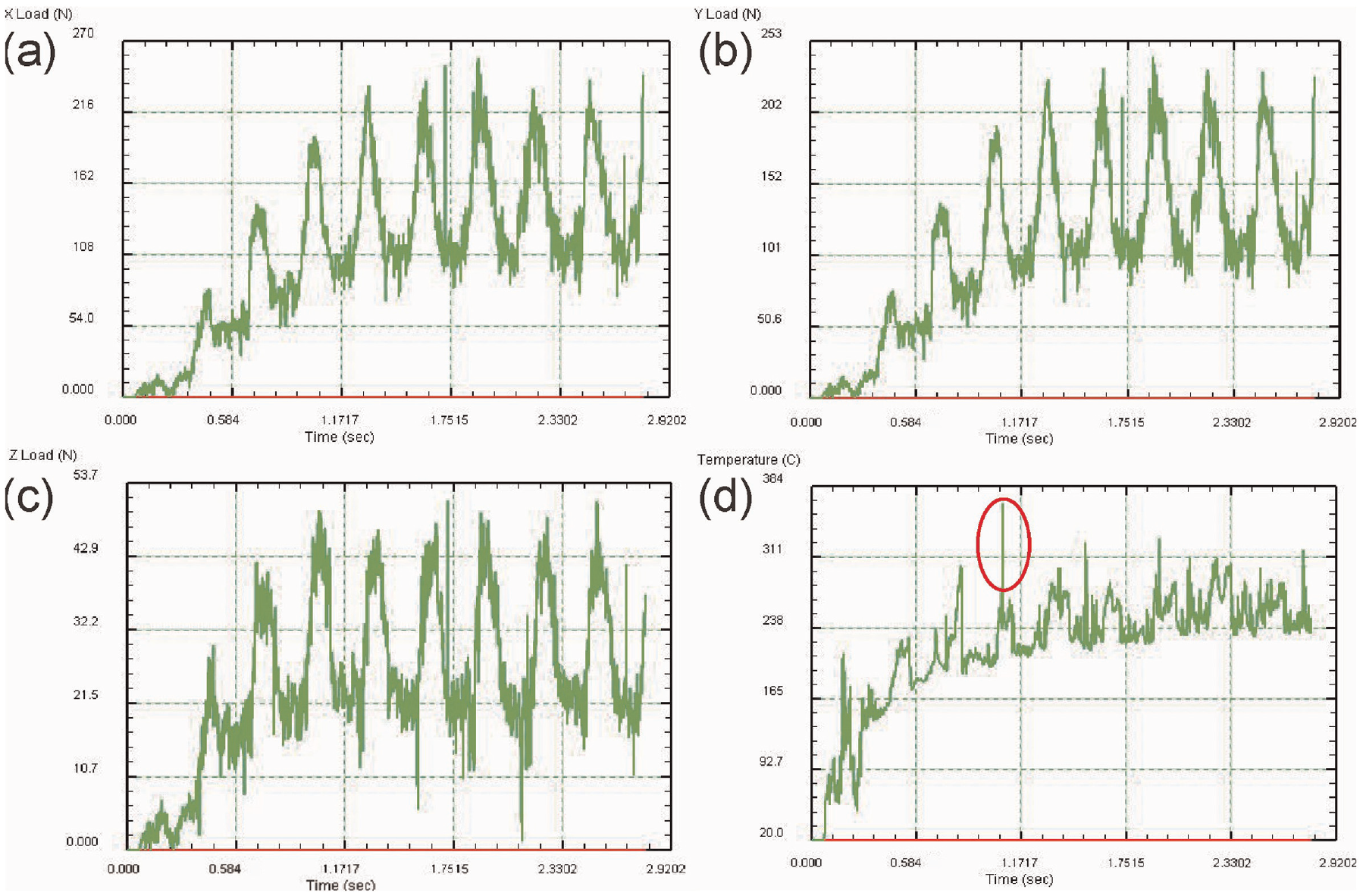
Simulation results of the first processing route: (a) cutting force in the X direction, (b) cutting force in the Y direction, (c) cutting force in the Z direction, and (d) cutting temperature.

Figure 13.

Simulation results of the second processing route: (a) cutting force in the X direction, (b) cutting force in the Y direction, (c) cutting force in the Z direction, and (d) cutting temperature.

The arithmetic mean difference of the contour, or, within the range of the sampling length L, the arithmetic mean of the absolute value of the distance from each point on the contour curve to the contour centerline, is the physical definition of surface roughness Ra. Through simulation, the working conditions of the workpiece surface are determined, the node coordinates of the machined surface are computed, and the formula can be used to determine the surface roughness of the simulation result.⁴⁴ The equation (3) takes M as the total number of samples of node coordinates, Z(i) as the value of the sample node coordinates in the Z direction, and −Z as the arithmetic mean of these node coordinates in the Z direction. The average of the surface roughness at each site determines the final surface roughness.

Ra = \frac{1}{M} \sum_{I = 1}^{M} [Z (i) - - Z]

(3)

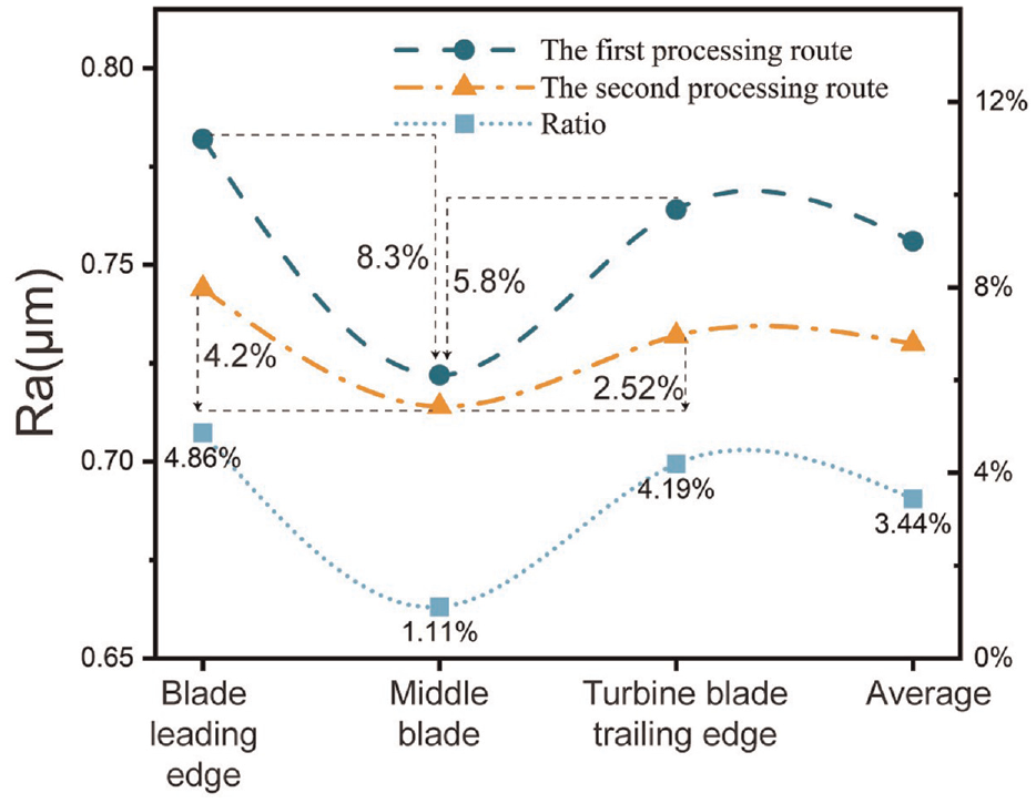
The blade is detached from the impeller, and the Z-axis node coordinates for the three locations of the blade leading edge, blade middle, and blade trailing edge are taken as indicated in the Figure 14 in order to better reflect the effect of two different finishing routes on the surface roughness of the blade. To determine the surface roughness value at three distinct points, enter the Z-axis node coordinates of each position into the equation (3). The final blade surface roughness value is determined by taking the arithmetic mean of the three places, as seen in the Figure 15 that indicates the blade processed by the first processing route had surface roughness values greater than those of the blade processed by the second processing route at the leading edge, middle section, and trailing edge. Following processing by the second processing method, the overall blade surface roughness value is approximately 3.44% less than that by the first processing route. Consequently, in fixed profile milling, it is preferable to control the tool axis to the designated plane normal rather than to the smooth interpolation vector in variable profile milling. The blade surface is flat and smooth, and the overall variation in the blade surface roughness value is stable. The blade surface roughness for the first processing route has a trend of initially dropping and then increasing, meaning that the leading edge of the blade has the highest roughness value, followed by the trailing edge, and the middle of the blade which have the lowest value. The more curved the surface to be machined, the more noticeable the overcutting phenomenon will be in the tool path during the machining process while the cutting parameters are fixed. A greater residual height and a smaller tool path density will result in a higher surface roughness value. On the other hand, for the second processing route, overcutting in the tool path may be successfully reduced by controlling the tool axis to the designated plane normal direction in fixed contour milling, especially in components with higher curvatures of the blade’s leading and trailing edge. At this point, surface roughness value will drop due to a decrease in residual height and an increase in tool path density. Therefore, it is required to adequately lower the feed per tooth, reduce the cutting speed, or use the “segmented and sub-regional cutting” processing method when processing large curvature curved surfaces in order to reduce surface roughness. Following the second processing approach, the leading and trailing edges of the blades have surface roughness differences of just 4.2% and 2.52% from the middle of the blade. Therefore, the second finishing route is preferable in terms of the surface roughness of the blade after processing.

Figure 14.

Divide blades.

Figure 15.

Values of surface roughness at three places.

Experimental verification of blade surface roughness

Processing the titanium alloy blank on the JD-U200A vertical double DD direct drive cradle type five-axis machining center as shown in the Figure 16(a) involves using the two finishing route CNC programs that have been precompiled. The titanium alloy open-type integrated micro impeller is CNC machined after the blank is roughed, the flow channel is roughed, the blades are finished, and other procedures are completed. The flat bottom milling cutter for roughing, the ball end milling cutter for finishing, and the finished impeller, are all depicted in the Figure 16(b) to (d). The residual micro-geometric shape on the workpiece’s surface can be represented by two and three-dimensional diagrams, and the surface topography of the workpiece can directly reflect the micro-geometric shape of the surface.⁴⁵ The ZYGO white light interferometer from AMETEK, which is depicted in the Figure 17(a), was utilized in this experiment to measure the workpiece’s surface topography. The following blade morphologies were measured in turn: the leading edge region, the intermediate region, the trailing edge region, and the overall morphology of the blade as indicated in the Figures 18 and 19. These include the following: Sa stands for the three-dimensional contour surface’s arithmetic mean deviation, Sq for the surface’s root mean square deviation, and Sz for the surface’s maximum height.

Figure 16.

Experimental processing system: (a) JD-U200A five-axis machining center, (b) The flat bottom milling cutter, (c) The ball end milling cutter and (d) Workpiece

Figure 17.

Surface topography measurement system: (a) ZYGO white light interferometer and (b) measurement system.

Figure 18.

The overall morphology of the blade: (a)(d) three-dimensional morphology, (b)(e) two-dimensional morphology, (c)(f) micromorphology, (a)(b)(c) first finishing routes, and (d)(e)(f) second finishing routes.

Figure 19.

Micromorphology: (a)(d) blade leading edge, (b)(e) middle blade, (c)(f) blade trailing edge, (a)(b)(c) first finishing routes, and (d)(e)(f) second finishing routes.

The Figure 18 illustrates the overall shape of the impeller surface as determined by a 20× white light interferometer microscope objective. Throughout the entire impeller processed using the first finishing routes, the average surface roughness is 0.772 and throughout the entire impeller processed using the second finishing routes, the average surface roughness is 0.749, both are greater than the surface roughness values obtained based on finite element analysis. The analysis is justified by the following: as cutting processing advances, the tool’s (cutting edge’s) wear failure model is no longer just the simple elastic-plastic deformation determined by finite element analysis, but is instead accompanied by a complex thermodynamic coupling process; in other words, the primary factors influencing surface roughness within a given range are the cutting force and the cutting heat. Wear on the tool will lower the cutting force when the cutting parameters remain constant. At this point, the surface roughness, burr generation, and residual height of the machined surface will all rise; The initial metal cutting process may eventually give way to a metal grinding process as the cutting continues. Numerous pieces of literature⁴⁶ have shown that the same workpiece’s surface roughness after grinding is less than its surface accuracy after cutting. On the other hand, the machining surface may be ablated, the cutting parameters remain constant, the cutting heat will rise, and the surface roughness will rise during the CNC machining process. But generally speaking, there is not much of a difference between the surface roughness value determined experimentally and the value derived by finite element analysis – both are less than 5%. As a result, the surface roughness value derived from finite element analysis can precisely represent the workpiece’s surface roughness.

It is evident from the Figure 19 that the surface morphology of the blade’s leading edge area, middle area, and trailing edge area was determined using a 20× white light interferometer microscope objective. Following the second finishing path, there is less residual height, less burrs, and less surface roughness in the surface topography of the blade leading edge area and blade trailing edge area. Both the surface roughness and surface morphology of the blade’s central section are similarly.

Establishment of surface roughness prediction model

Due to its small geometric size, the integrated micro impeller is a type of micro structural item that places significant requirements on the planning of cutting paths and the calculation of cutting parameters. As a result, the precise prediction and control of surface roughness of micro-structured parts depend greatly on the thoughtful selection of cutting settings and processing pathways.⁴⁷ Therefore, this study conducts a comparative analysis between the surface roughness prediction model established based on mathematical and statistical principles (Box-Behnken design response surface method) and the surface roughness prediction model established based on machine learning and artificial intelligence (Back Propagation Neural Networks, Support Vector Machine). As shown in the Figure 20.

Figure 20.

Establishment of experiment and prediction model.

Establishment and analysis of surface roughness prediction model based on response surface method

Mathematics and statistics are combined in the second-order response surface method based on central composite design. The benefits of the second-order response surface approach are low test numbers, continuity, rotatability, and resilience of the model.⁴⁸ It is frequently used to address real-world issues involving multi-factor interaction because its response prediction results can also approximate the true response surface and produce the optimum prediction effect.⁴⁹ Equation (4) illustrates how the second-order response surface approach expands the Taylor expansion for a single variable to multiple variables⁵⁰:

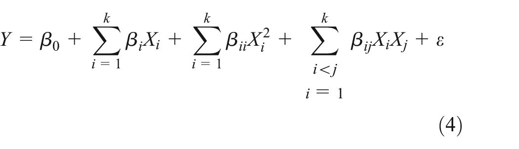
Y = β_{0} + \sum_{i = 1}^{k} β_{i} X_{i} + \sum_{i = 1}^{k} β_{i i} X_{i}^{2} + \sum_{\begin{array}{l} i < j \\ i = 1 \end{array}}^{k} β_{i j} X_{i} X_{j} + ε

(4)

In the equation (4), Y is the response target, which is the roughness value Ra in this article; X_i and X_j are model input variables; k is the number of input variables, k = 3; β_i and β_ii are the coefficients of linear effect and second-order effect respectively; β_ij is the coefficient of interaction between parameters X_i and X_j; ε is the normal random error term. The second-order response surface model of three factors can be written as the equation (5):

\begin{matrix} Y = β_{0} + β_{1} X_{1} + β_{2} X_{2} + β_{3} X_{3} \\ + β_{11} X_{1} X_{1} + β_{12} X_{1} X_{2} + β_{13} X_{1} X_{3} \\ + β_{21} X_{2} X_{1} + β_{22} X_{2} X_{2} + β_{23} X_{2} X_{3} \\ + β_{31} X_{3} X_{1} + β_{32} X_{3} X_{2} + β_{33} X_{3} X_{3} + ε \end{matrix}

(5)

The surface roughness of the workpiece during the metal cutting process is influenced by several elements, such as cooling and lubrication systems, cutting parameters, tool parameters, tool surface coating performance, etc.⁵¹ Numerous researchers have discovered that the cutting settings have the greatest influence on the workpiece’s surface roughness. Maintaining the stability of cutting conditions is facilitated by the reasonable selection of cutting parameters.⁵² A common experiment based on response surface theory is the Box-Behnken design (BBD) experiment, which examines the connection between material processing properties and cutting parameters.⁵³ Using the three process parameters of cutting depth, feed per tooth, and cutting speed, a three-factor and three-level BBD experiment was set up to further investigate the relationship between each parameter and the response target. As an illustration, choosing process settings appropriate for cutting micro structural elements using the second finishing route for processing blades.⁵⁴ The experimental level table is shown in the Table 1. Variance analysis should be performed on the BDD experimental data; the findings are displayed in the Table 2.

Table 1.

BBD experimental factors and level table.

Factors	Level 1	Leve 2	Level 3
a_p (mm)	0.05	0.07	0.09
f_z (mm)	0.05	0.06	0.07
v_c (m/min)	47.1239	51.8363	56.5487

Table 2.

The ANOVA of BBD experiment results.

Source	Sum of squares	DOF	Mean square	F-value	p-Value, Prob > F	For 95% confidence level
Model	0.041307	9	0.004589	16.955737	0.000583	Significant
Residual	0.001895	7	0.000271
Lack of fit	0.001180	3	0.000393	2.201082	0.230458	Not significant
Pure error	0.000715	4	0.000179
Adj R² = 0.8998
Pred R² = 0.5371
Adeq precision = 16.008

It can be seen from the variance analysis Table 2 that the p-value of the regression term of the second-order response surface equation is 0.000583 < 0.05, and the p-value of the lack-of-fit term is 0.230458 > 0.05; Adequate precision estimates the signal to noise ratio and an A ratio exceeding 4 is desirable. The measurement of the signal to noise ratio resulted in 16.008, respectively, implying an adequate precision ratio. The regression model developed for the experiment is significant and trustworthy, according to the variance analysis results. The response surface equation of the actual factor levels to surface roughness is produced after transforming the encoded factor levels into actual level values, as shown in equation (6).

\begin{matrix} R_{a} = 3.12129 + 14.4775 * a_{p} + 52.805 * f_{z} - 0.19002 * v_{c} \\ - 112.5 * a_{p} * f_{z} + 0.058357 * a_{p} * v_{c} - 0.66845 * f_{z} * v_{c} \\ - 66.625 * a_{p}^{2} - 76.5 * f_{z}^{2} + 0.00226734 * v_{c}^{2} \end{matrix}

(6)

The significance of the effect of milling parameters on surface roughness under current cutting conditions is graded as follows based on a comparison of the absolute values of the response surface equation’s coefficients. (1) The significance of the linear effect from large to small is: feed per tooth f_z, cutting depth a_p, cutting speed v_c; (2) The significance of the interaction effects from large to small is a_pf_z interaction, f_zv_c interaction, and a_pv_c interaction; (3) The significance of the secondary effects from large to small is f_z², a_p², v_c².

The response surface diagram of the interaction is created using the Design-Expert program in accordance with the BBD experimental results, shown in the Figure 21.

(1) The Figure 21(a) illustrates how surface roughness increases with increasing cutting depth and feed per tooth at a cutting speed of 51.8363 m/min. The impact of cutting depth on surface roughness is greater than that of feed per tooth, and the minimum value of surface roughness can be achieved at the minimum cutting depth and minimum feed per tooth.

(2) The Figure 21(b) illustrates how surface roughness first decreases and then increases with increasing cutting speed when the feed rate per tooth is 0.06 mm. Greater or lesser cutting speeds during the microstructural part-cutting process will result in a rougher surface. In large cutting speeds, there will be more vibration and roughness in the blade. The roughness will increase and the metal chips cannot be instantly separated at low cutting speeds. Selecting the cutting depth at the minimum of 0.05 mm and the speed of close to 51 m/min will result in a surface roughness of around 0.53 μm. Thus, in order to lessen the impact of surface roughness, the cutting speed must be chosen suitably.

(3) The Figure 21(c) illustrates how surface roughness first lowers and subsequently grows with increasing cutting speed when the cutting depth is set at 0.07 mm. Surface roughness increases with an increase in feed per tooth when the cutting speed is less than 48 m/min; however, surface roughness reduces with an increase in feed per tooth when the cutting speed exceeds 56 m/min, At the moment, the cutting speed and feed per tooth can achieve dynamic balance. Surface roughness can be efficiently decreased by increasing both the cutting speed and feed per tooth at the same time. However, this will result in increased cutting force, cutting temperature, tool wear, and extra expenses.

Figure 21.

Response surface diagram of interaction: (a) interaction f_z with a_p, (b) interaction v_c with a_p, and (c) interaction v_c with f_z.

Establishment and analysis of surface roughness prediction model based on support vector machine

Many academics have addressed the application of artificial intelligence techniques like neural networks to build multi-factor nonlinear mapping relationships because surface roughness and cutting parameters offer a nonlinear mapping connection.⁵⁵ One kind of supervised machine learning method among them is the Support Vector Machine (SVM) algorithm. It has been extensively utilized in turning, milling, and grinding to predict surface roughness data. It can avoid the issues of overfitting and lengthy training times of the BP neural network model, thanks to its benefits of rapid learning and excellent generalization.⁵⁶

Therefore, in order to further verify the prediction effect of the model, the surface roughness prediction data, SVM model prediction data, and BP neural network model prediction data calculated by the equation (6) are compared with the experimental measured data. The analysis results are shown in the Figure 22.

Figure 22.

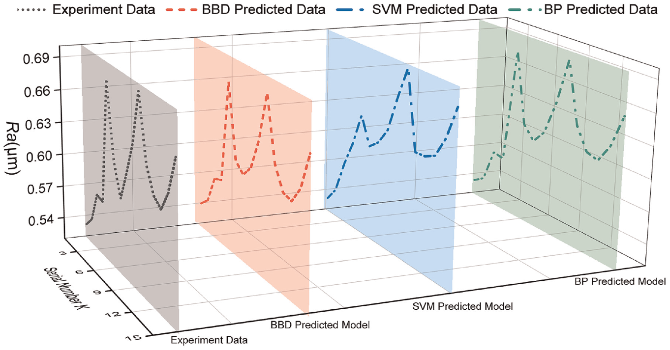
Experiment data and predicted data.

It can be concluded from the Figure 22 that the average error between the calculated surface roughness prediction data and the experimental data is 1.1%, the average error between the SVM model prediction data and the experimental data is 11.9%, and the average error between the BP neural network model prediction data and the experimental data is 25.1%. The thorough analysis is conducted because: 15 sets of cutting trials provide the data for the three surface roughness models. (1) The acceptable selection range of cutting parameters has been established in the earlier study. The prediction model established mathematical and statistical methods may more accurately capture the multi-factor nonlinear mapping connection between samples inside a fixed sample space. Furthermore, the response surface graphic clearly shows the interaction relationship between cutting parameters and target criteria. (2) The multi-factor nonlinear mapping connection between samples may also be reflected in the prediction model constructed using machine learning and artificial intelligence; however, the sample space is limited since the cutting parameter selection range has already been established. Low prediction accuracy results from the inability to exhibit machine learning’s strong prediction and generalization skills. (3) The SVM prediction model and the BP neural network prediction model still have certain shortcomings in the small sample space, such as slow running speed, easy to fall into local optimality,⁵⁷ etc., and the interactive relationship between cutting parameters and target factors cannot be clearly obtained. Therefore, it is difficult to achieve accurate prediction of data. (4) In order to further improve the accuracy of the prediction model based on machine learning and artificial intelligence, the number of sample spaces should be increased and the prediction model should be optimized accordingly, so as to increase the training speed and prevent it from falling into local optimality.

Conclusion

Because of its complex overall shape and difficult material, the open integral micro impeller of titanium alloy has always presented a challenge for engineers working in the field of multi-axis CNC machining. Given the technical challenges associated with processing micro impellers, such as high material removal rates, large blade curvatures, and narrow flow channels. Our study has added new contributions to the body of current knowledge in the following ways: Creating two different and suitable finishing paths using the NX2212 software. Importing the finishing paths into DEFORM-3D in the form of point sets. Calculating the surface roughness value based on mathematical principles and verify it experimentally. Establishing a surface roughness prediction model based on mathematical principles and machine learning. This article:

(1) Firstly, the CAM software NX2212 modeling module creates the 3D model of the open integral micro impeller. Next, two distinct processing routes are utilized to complete the blade. The virtual machine tool simulation module verifies the accuracy and safety of the processing route. Finally, the numerical control program is exported in the post-processing module, and MATLAB software simulates and synthesizes the data. It is possible to infer from the fitting curve that the “one-cutter flow” machining mode has a greater cutting efficiency, while the “segmentation cutting” machining mode has a higher blade precision.

(2) Secondly, the tool and the workpiece are positioned in the NX2212 assembly module. The simulation environment variables were set, the STL format was imported into DEFORM-3D, a finite element analysis program, and the blade surface roughness was computed based on the simulation outcomes.

(3) Additionally, the machine operates the two types of finishing trajectories that were initially created, and a white light interferometer measures the surface morphology of the micro impeller entity. The findings demonstrate that there is extremely little variation, both of which are less than 5% between the surface roughness determined by the finite element analysis software and the surface roughness measured by the experiment.

(4) Finally, a three-factor and three-level BBD experiment based on the second-order response surface approach was constructed in order to further improve the prediction accuracy of the surface roughness of micro-structural parts. The findings demonstrate that, within a suitable cutting parameters range, the impact of feed per tooth on surface roughness is greater than the effects of cutting depth and speed. Surface roughness will increase with larger or smaller cutting speeds; yet, surface roughness can also be decreased with higher cutting speeds and feed rates per tooth. Surface roughness can be accurately predicted and controlled by the second-order response surface method prediction model, which is based on mathematical and statistical principles. It has higher confidence and more significant regression than the prediction model based on machine learning and artificial intelligence.

Footnotes

Handling Editor: Chenhui Liang

Author contributions

HaiYue Zhao performed the data analyses and wrote the manuscript; Yan Cao contributed to the conception of the study; JunDe Guo contributed significantly analysis and manuscript preparation; Biao Sun directed the experiment; Nan Geng performed the experiment.

Declaration of conflicting interests

The author(s) declared no potential conflicts of interest with respect to the research, authorship, and/or publication of this article.

Funding

The author(s) disclosed receipt of the following financial support for the research, authorship, and/or publication of this article: This research was funded by This research was funded by National Natural Science Foundation of China (Grant: 52275508), Shaanxi Innovation Capability Support Plan (Grant: 2022PT-02), Xi’an Science and Technology Project (Grant: 2020KJRC0032), Research on the development of practical skills of professional degree students of Chinese Society for Degree and Postgraduate Education (Grant: 2020ZDB89).

ORCID iD

Yan Cao

Availability of data code and materials

Most of the data are presented in the manuscript, and a detailed sample will be provided upon request through from the corresponding author.

References

Chong

Zhu

. Innovative technologies in manufacturing, mechanics and smart civil infrastructure. Int J Smart Nano Mater 2018; 9: 261–278.

Vafadar

Guzzomi

Rassau

, et al. Advances in metal additive manufacturing: a review of common processes, industrial applications, and current challenges. Appl Sci Basel 2021; 11: 1213.

. Towards green innovation by China’s industrial policy: evidence from made in China 2025. Front Environ Sci 2022; 10: 924250.

Gao

Wang

, et al. Application of green design and manufacturing in mechanical engineering: education, scientific research, and practice. Sustainability 2022; 14: 237.

Qiu

Guo

. Current situation and development trend of titanium metal industry in China. Int J Miner Metall Mater 2022; 29: 599–610.

Cui

Zhao

, et al. Titanium alloy production technology, market prospects and industry development. Mater Des 2011; 32: 1684–1691.

Gao

Wang

Yang

, et al. Heterogeneous deformation behavior of hybrid manufactured TC11 titanium alloy via directed energy deposition. Mater Sci Eng Struct Mater Prop Microstruct Process 2023; 867: 144728.

Yang

Fan

Sun

, et al. Recent developments in plastic forming technology of titanium alloys. Sci China Technol Sci 2011; 54: 490–501.

Hewitt

Davies

Thomas

, et al. Titanium alloy developments for aeroengine fan systems. Mater Sci Technol 2014; 30: 1919–1924.

10.

Zhang

. Effects of cutting conditions on the milling process of titanium alloy Ti6Al4V. Int J Adv Manuf Technol 2015; 77: 2235–2240.

11.

Lee

J-N

Chen

H-S

Kung

H-K

. Geometric modeling and five-axis NC machining for centrifugal impeller. In: International conference on advanced design and manufacturing engineering (ADME 2011), Guangzhou, China, 16–18 September 2011, pp.1556+.

12.

Wang

Zheng

, et al. Experimental and simulation study on chatter stability region of integral impeller with non-uniform allowance. Sci Prog 2020; 103:420933418. https://doi.org/10.1177/0036850420933418

13.

Ding

Chu

Guan

, et al. Research on machining error prediction of open blade under dynamic loading. Ferroelectrics 2022; 593: 10–25.

14.

Song

Liu

, et al. A generalized cutting force model for five-axis milling processes. Proc IMechE, Part B J: Engineering Manufacture 2019; 233: 3–17.

15.

Chen

Wang

, et al. Tool path strategy and cutting process monitoring in intelligent machining. Front Mech Eng 2018; 13: 232–242.

16.

Liang

Wang

. A new rough machining approach for a ruled surface impeller. In: International conference on chemical, mechanical and materials engineering (CMME 2011), Guangzhou, China, 8–10 July 2011, pp.53+.

17.

Liu

Jia

, et al. Interpolation using non-uniform rational B-spline for the smooth milling of ruled-surface impeller blades. Proc IMechE, Part B: J Engineering Manufacture 2015; 229: 1118–1130.

18.

Stratogiannis

Galanis

Karkalos

, et al. Optimization of the manufacturing strategy, machining conditions, and finishing of a radial impeller. Machines 2020; 8: 1.

19.

Han

Zhang

, et al. A dynamic synchronous optimisation method of tool sequence selection and multi-state process models depth distribution for high efficiency machining. Int J Prod Res 2020; 58: 6145–6158.

20.

Wang

, et al. Research into dynamic error optimization method of impeller blade machining based on digital-twin technology. Machines 2023; 11: 697.

21.

Soori

Asmael

. Minimization of deflection error in five axis milling of impeller blades. Facta Univ Ser Mech Eng 2023; 21: 175–190.

22.

Feng

Wei

Wang

, et al. Tool path planning for five-axis U-pass milling of an impeller. Int J Adv Manuf Technol 2021; 117: 3379–3391.

23.

Payaminia

Moslemian

Younespour

, et al. Evaluating the effect of repeated use of milling burs on surface roughness and adaptation of digitally fabricated ceramic veneers. Heliyon 2021; 7: e06896.

24.

Zou

Fang

, et al. Roughness estimation of high-precision surfaces from line blur functions of reflective images. Measurement 2021; 182: 109677.

25.

Ngerntong

Butdee

. Surface roughness prediction with chip morphology using fuzzy logic on milling machine. In: 10th international conference of materials processing and characterization (ICMPC), GLA University, Mathura, India, 21–23 February 2020, pp.2357–2362.

26.

Yang

Zheng

. A prediction model for titanium alloy surface roughness when milling with micro-textured ball-end cutters at different workpiece inclination angles. Int J Adv Manuf Technol 2019; 100: 2115–2122.

27.

Savas

Ozay

Ballikaya

. Experimental investigation of cutting parameters in machining of 100Cr6 with tangential turn-milling method. Adv Manuf 2016; 4: 97–104.

28.

Zhang

Cheng

Xia

, et al. Influence of laser shot peening parameters on the surface hardness and roughness of 7075 aluminum alloy. Mater Sci Forum 2018; 4653: 83–88.

29.

Lin

Y-C

K-D

Shih

W-C

, et al. Prediction of surface roughness based on cutting parameters and machining vibration in end milling using regression method and artificial neural network. Appl Sci Basel 2020; 10: 3941.

30.

Liu

, et al. Roughness prediction model of milling noise-vibration-surface texture multi-dimensional feature fusion for N6 nickel metal. J Manuf Processes 2022; 79: 166–176.

31.

Nouhi

Pour

. Prediction of surface roughness of various machining processes by a hybrid algorithm including time series analysis, wavelet transform and multi view embedding. Measurement 2021; 184: 109904.

32.

Deng

, et al. On-line surface roughness classification for multiple CNC milling conditions based on transfer learning and neural network. Int J Adv Manuf Technol 2023; 128: 1063–1076.

33.

Jiang

Lin

, et al. Prediction and compensation strategy of contour error in multi-axis motion system. Int J Adv Manuf Technol 2022; 119: 163–175.

34.

de Oliveira

de Souza

Diniz

. Evaluating the influences of the cutting parameters on the surface roughness and form errors in 4-axis milling of thin-walled free-form parts of AISI H13 steel. J Braz Soc Mech Sci Eng 2018; 40: 334.

35.

Zhang

Zhou

, et al. A digital twin defined autonomous milling process towards the online optimal control of milling deformation for thin-walled parts. Int J Adv Manuf Technol 2023; 124: 2847–2861.

36.

Zhao

Cao

Bai

, et al. Numerical simulation and tool parameters optimization of aluminum alloy transmission intermediate shell. Sci Rep 2024; 14: 4241.

37.

Zhang

Zhou

, et al. A multi-access edge computing enabled framework for the construction of a knowledge-sharing intelligent machine tool swarm in Industry 4.0. J Manuf Syst 2023; 66: 56–70.

38.

Wang

Zhu

C-D

Liu

, et al. Research on plastic deformation law and forming technology of rotary forging with multi-cone rolls. Adv Mech Eng 2021; 13: 16878140211008759.

39.

Mali

Agrahari

Gupta

TVK

. FE based simulation and experimental validation of forces in dry turning of aluminium 7075. In: International conference on materials and manufacturing methods (MMM), Tiruchirapalli, India, 5–7 July 2019, pp.2319–2323.

40.

Maity

Pradhan

. Investigation of FEM simulation of machining of titanium alloy using microgroove cutting insert. Silicon 2018; 10: 1949–1959.

41.

Wang

Cao

Gorbachev

, et al. Research on conventional and high-speed machining cutting force of 7075-T6 aluminum alloy based on finite element modeling and simulation. Metals 2022; 12: 1395.

42.

Shen

, et al. Surface characteristics and corrosion behavior of TC11 titanium alloy strengthened by ultrasonic roller burnishing at room and medium temperature. J Mater Res Technol 2020; 9: 8172–8185.

43.

Wang

Cao

Yao

, et al. Dynamic simulation and experimental study of cutting force by rake angle of multi-axis high-speed ball-end milling tool. Int J Adv Manuf Technol 2022; 122: 377–390.

44.

Yang

Wang

Kang

. Finite element simulation of surface roughness in diamond turning of spherical surfaces. J Manuf Processes 2018; 31: 768–775.

45.

Huang

Deng

, et al. Experimental and numerical investigation on thin sheet metal roll forming process of micro channels with high aspect ratio. Int J Adv Manuf Technol 2019; 100: 117–129.

46.

Wen

Gong

. Simulation and experimental research on grinding force and grinding surface quality of TiC-coated micro-grinding tools. Int J Adv Manuf Technol 2023; 128: 1337–1351.

47.

Sun

Hou

, et al. Numerical simulation of micro-element cutting and milling force prediction in micro ball-end milling. Int J Adv Manuf Technol 2023; 125: 2305–2322.

48.

Jia

Wang

, et al. The effect of cutting parameters on micro-hardness and the prediction of Vickers hardness based on a response surface methodology for micro-milling Inconel 718. Measurement 2019; 140: 56–62.

49.

Chuangwen

Ting

Xiangbin

, et al. Experimental tests and empirical models of the cutting force and surface roughness when cutting 1Cr13 martensitic stainless steel with a coated carbide tool. Adv Mech Eng 2016; 8: 1687814016673753.

50.

Duc

Giang

Dai

, et al. An experimental study on the effect of tool geometry on tool wear and surface roughness in hard turning. Adv Mech Eng 2014; 12: 1687814020959885.

51.

Movahedi

Mokhtari Homami

Akhavan

. A new approach of wear mechanism map in turning inconel718 with PVD-coated inserts using advanced techniques. Iran J Sci Technol Trans Mech Eng 2020; 44: 1091–1102.

52.

da Costa Castanhera

Diniz

. Cutting forces, surface roughness and tool life in high-speed milling of hardened steel convex surface. J Braz Soc Mech Sci Eng 2017; 39: 3555–3570.

53.

Ozturk

Kahraman

. Modeling and optimization of machining parameters during grinding of flat glass using response surface methodology and probabilistic uncertainty analysis based on Monte Carlo simulation. Measurement 2019; 145: 274–291.

54.

Fan

H-Z

Wang

, et al. An efficient five-axis machining method of centrifugal impeller based on regional milling. Int J Adv Manuf Technol 2016; 87: 789–799.

55.

Patra

Jha

Szalay

, et al. Artificial neural network based tool condition monitoring in micro mechanical peck drilling using thrust force signals. Precis Eng 2017; 48: 279–291.

56.

Wang

Meng

Zhao

, et al. Prediction of machine tool condition using support vector machine. J Phys Conf Ser 2011; 305: 012113.

57.

Aich

Banerjee

. Modeling of EDM responses by support vector machine regression with parameters selected by particle swarm optimization. Appl Math Modell 2014; 38: 2800–2818.

Multi-axis CNC finishing and surface roughness prediction of TC11 titanium alloy open integral micro impeller

Abstract

Keywords

Introduction

Multi-axis CNC finishing process of open integral micro impeller

Finishing process of open integral micro impeller

Surface roughness acquisition and experimental verification based on finite element analysis

Establishment of finite element simulation model based on DEFORM-3D

Experimental verification of blade surface roughness

Establishment of surface roughness prediction model

Establishment and analysis of surface roughness prediction model based on response surface method

Establishment and analysis of surface roughness prediction model based on support vector machine

Conclusion

Footnotes

Author contributions

Declaration of conflicting interests

Funding

ORCID iD

Availability of data code and materials

References