Sage Journals: Discover world-class research

Abstract

Gaussian road profile is widely used to study vehicle response and fatigue damage potential, while field measured road profile often is non-Gaussian. In this paper, a new amplitude modulation method which has full control of cutoff frequency (denoted as Wcut) and amplitude of the amplitude modulation signal is firstly presented to synthesize non-Gaussian road profile with different kurtosis. The forced response of a quarter vehicle under non-Gaussian road profile excitation is then calculated using the ramp invariant digital filter method. The relationship between the vehicle response characteristics and the kurtosis of input non-Gaussian road profile are developed. A case study is used to verify the proposed method. The results show that a small Wcut should be selected so that the high kurtosis of the non-Gaussian road profile is correctly transferred to the vehicle response. The FDS of the vehicle response increases over the entire frequency range as the kurtosis of the input road profile increases.

Keywords

Non-Gaussian road profile cutoff frequency kurtosis fatigue damage

Introduction

Vibration test is performed on vehicles in order to achieve comfort and safety requirements. As a major source of vehicle vibration and fatigue damage, road surface roughness is usually characterized by Power Spectral Density (PSD),¹ with an assumption that the road roughness follows a Gaussian distribution. In practice, however, field measured data are usually non-Gaussian,^2,3 which may result in non-Gaussian response and a shorter fatigue life.⁴

To simulate the non-Gaussian random vibration caused by road roughness, several methods have been proposed to generate non-Gaussian signals with given PSD and kurtosis.^5,6 Among these methods, the amplitude modulation method was firstly developed by Smallwood,⁷ in which a Gaussian signal was generated and then multiplied with an amplitude modulation signal (AMS) that was independent of the Gaussian signal. The kurtosis of a non-Gaussian signal generated using this method was governed by the AMS. Different methods were proposed to construct the AMS, including Beta distribution,⁷ Gamma distribution,⁸ Weibull distribution,⁹ etc. Xu et al.¹⁰ indicated that when modeling the AMS by Weibull distribution, inappropriate determination of the number of bursts may lead to distortion of the original PSD, resulting in an ineffective fatigue test.

Under non-Gaussian road profile excitation, Yang et al.¹¹ performed fatigue life analysis of vehicle systems based on polynomial chaos expansion, Karhunen-Loeve expansion and quasi Monte Carlo approach. However, to achieve an effective non-Gaussian fatigue test, the high kurtosis of the simulated excitation has to be transferred into the structural response.¹² Tao and Cheng¹³ studied the stress response of Multi-degree of freedom system under non-Gaussian signal excitation, and analyzed the stress response under non-Gaussian signal excitation from the perspectives of kurtosis and fatigue damage. Kihm et al.¹⁴ studied the influence of the kurtosis of the excitation signal on the kurtosis of system response, and found that the high kurtosis of non-stationary non-Gaussian excitation is easier to transmit in the system. Hosoyama et al.¹⁵ has shown that when the natural frequency reaches a specific value, an increase in the excitation kurtosis will lead to a significantly increase in the response kurtosis. Steinwolf et al.⁴ presented two methods to generate high kurtosis random vibration signal. The Fatigue damage spectrum (FDS) was used for an evaluation of the time to failure. But only one point of the FDS curve was considered to evaluate the proposed method. The problem of the aforementioned methods is that the relationship between the kurtosis transmission and the construction method of AMS is not clear. The effects of AMS parameters on the response kurtosis and the whole frequency range of FDS are not studied.

The main idea of this study is to firstly present a new amplitude modulation method to synthesize non-Gaussian road profile. The high kurtosis transmission is ensured by frequency control and cumulative distribution function (CDF) transformation of the AMS. The characteristics of vehicle response under non-Gaussian road profile excitation, including the kurtosis and FDS, are finally studied to show the effects of cutoff frequency of AMS and input kurtosis on the response.

The remainder of this study is organized as follows. In Section “Theoretical background,” the theoretical background of Gaussian and non-Gaussian road profile, vehicle model, and the FDS calculation process are presented. In Section “Synthesis of non-Gaussian road profile,” a novel AMS modeling method is presented to synthesize non-Gaussian road profile. In Section “Case study,” simulated data are used to validate the proposed approach. Effects of cutoff frequency of AMS and input kurtosis on the vehicle response and FDS are studied. Finally, the conclusions are presented in Section “Conclusion.”

Theoretical background

Gaussian and non-Gaussian road profile

A road profile z(x) describes the road roughness as a function of distance. Stationary Gaussian road profiles have been extensively used as models for road roughness, which can be described by a displacement PSD¹:

G (Ω) = G_{0} \cdot {(\frac{Ω}{Ω_{0}})}^{- w}

(1)

where, Ω is the spatial angular frequency, Ω₀ is the reference spatial angular frequency, and Ω₀ = 1 rad/m; G₀ is the roughness coefficient and G₀ = 1.e⁻⁶ is a typical value; w is the slop of PSD on a loglog scale and a typical value is w = 2.

A typical Gaussian road profile is shown in Figure 1.

Figure 1.

Gaussian road profile.

The PDF of a Gaussian road profile with zero mean value is expressed as:

p (z) = \frac{1}{\sqrt{2 π} σ_{z}} e^{- \frac{z^{2}}{2 σ_{z}^{2}}}

(2)

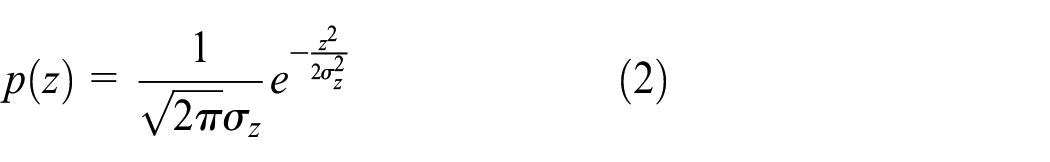
where, σ_z is the standard deviation:

σ_{z}^{2} = E [z^{2} (x)] = \int_{- \infty}^{\infty} z^{2} p (z) d z

(3)

However, field measured road profile often presents non-Gaussian characteristic. A measured road profile is shown in Figure 2. The data was measured on Swedish country road with a laser vehicle. The test setup is shown in Figure 3.

Figure 2.

Measured non-Gaussian road profile.

Figure 3.

Test vehicle and laser setup.

Kurtosis is used to identify whether a road profile is non-Gaussian:

K = \frac{m_{4}}{{σ_{z}}^{4}}

(4)

where, m₄ is the fourth order central moment:

m_{4} = \frac{1}{N} \sum_{i = 1}^{N} {(z_{i} - μ)}^{4}

(5)

μ is the mean value and N is the number of data sample.

A comparison of PDF of Gaussian and non-Gaussian road profile is shown in Figure 4. From Figure 4 we can see that a kurtosis value greater than 3 indicates wider tails. A wider tail indicates a higher probability of larger peak values, which leads to larger fatigue damage and faster failure.

Figure 4.

PDF comparison of Gaussian and non-Gaussian road profile.

Vehicle model

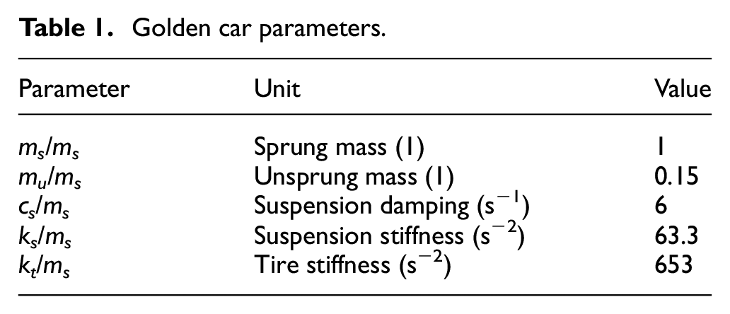
A golden car model,¹⁶ as shown in Figure 5, is used to calculate the vehicle response. All parameters are normalized to m_s and shown in Table 1.

Figure 5.

A golden car model.

Table 1.

Golden car parameters.

Parameter	Unit	Value
m _s/m_s	Sprung mass (1)	1
m _u/m_s	Unsprung mass (1)	0.15
c _s/m_s	Suspension damping (s⁻¹)	6
k _s/m_s	Suspension stiffness (s⁻²)	63.3
k _t/m_s	Tire stiffness (s⁻²)	653

The motion equation of the golden car model can be written as:

\begin{matrix} [\begin{matrix} m_{s} & 0 \\ 0 & m_{u} \end{matrix}] {\begin{matrix} {\overset{\cdot\cdot}{z}}_{s} (t) \\ {\overset{\cdot\cdot}{z}}_{u} (t) \end{matrix}} + [\begin{matrix} c_{s} & - c_{s} \\ - c_{s} & c_{s} \end{matrix}] {\begin{matrix} {\overset{\cdot}{z}}_{s} (t) \\ {\overset{\cdot}{z}}_{u} (t) \end{matrix}} \\ + [\begin{matrix} k_{s} & - k_{s} \\ - k_{s} & k_{s} + k_{t} \end{matrix}] {\begin{matrix} z_{s} (t) \\ z_{u} (t) \end{matrix}} = {\begin{matrix} 0 \\ k_{t} \cdot z (t) \end{matrix}} \end{matrix}

(6)

where, z_s(t) and z_u(t) are the vertical displacement of sprung and unsprung mass, respectively, z(t) is the road profile in time domain.

The ramp invariant digital filter method¹⁷ is used in this paper to calculate the vehicle response under Gaussian road profile and non-Gaussian road profile. To transform the road profile from spatial domain to time domain, a sampling frequency f_s in Hz can be calculated as:

f_{s} = \frac{v * 1000}{3600} \cdot f_{x} = \frac{v}{3.6} \cdot f_{x}

(7)

where, v is the vehicle speed in km/h, f_x is the number of data samples per meter.

Fatigue damage spectrum (FDS)

FDS is building on the use of the Basquin simplification of a Wöhler S/N curve and Miner’s rule for partial damage, as shown in Figure 6. The signal to be analyzed, usually given as acceleration, is fed to the base of a series of Single Degree of Freedom (SDOF) systems, defined by their resonance frequency f_n and quality factor Q, as shown in Figure 7.

Figure 6.

Calculation procedure of the FDS.

Figure 7.

Single degree of freedom systems for calculation of FDS.

The response of each SDOF system is analyzed with some cycle counting method, such as Rain Flow Cycle Count,¹⁸ giving the number of cycles for each response amplitude interval. The number of cycles is used to calculate the damage for the studied resonance frequency, using Miner’s rule. The plot of damage as function of SDOF resonance frequency defines the FDS.

D_{t} (f_{n}) = \sum_{i = 1}^{p} \frac{n_{i}}{N_{i}} = \sum_{i = 1}^{p} \frac{n_{i} S_{i}^{b}}{c}

(8)

where, n_i is the number of cycles at the stress level S_i (i = 1, 2, …, p), p is the number of stress levels considered, N_i is the fatigue life at the stress level, c is a constant, b is the fatigue index, D_t is the FDS in time domain.

Assuming stress is proportional to pseudo velocity:

S = k x_{pv}

(9)

where, the pseudo velocity can be calculated using a ramp invariant digital filter¹⁸:

x_{p v} = f i l t e r (b, a, x (t))

(10)

where, a and b the coefficients of the digital filter, x(t) is the input acceleration, filter is a MATLAB function.

Using equations (8)–(10), the FDS can be calculated as:

D_{t} (f_{n}) = \sum_{i = 1}^{p} \frac{n_{i}}{N_{i}} = \sum_{i = 1}^{p} \frac{n_{i} k^{b} x_{pv, i}^{b}}{c} = \frac{k^{b}}{c} \sum_{i = 1}^{p} n_{i} x_{pv, i}^{b}

(11)

Whereas for exact fatigue life predictions b, c, k, and Q have to be known explicitly, in practice their values may be unknown or difficult to estimate. In this case, it is possible to set b = 5, c = k = 1, Q = 10 and nevertheless use the FDS as an indicator to compare the damage potential of different vibration profiles.¹⁹ Using these parameters, the pseudo velocity FDS of sprung mass response under Gaussian and non-Gaussian road profile were calculated. Specifically, Gaussian and non-Gaussian road profile are used to excite the golden car model in Figure 5 and calculate the sprung mass response. The FDS is calculated using equations (8)–(11). To study the vehicle response under non-Gaussian road profile excitation, a new method to synthesize non-Gaussian road profile is presented in the next Chapter.

Synthesis of non-Gaussian road profile

The basic idea of amplitude modulation method is to generate the required non-Gaussian road profile z(x) by multiplying a Gaussian road profile g(x) with given PSD with a slowly varying Amplitude Modulation Signal (AMS) w(x):

z (x) = g (x) \cdot w (x)

(12)

where the AMS w(x) follows a Weibull distribution.

The AMS is scaled to have mean square one not to change the scale of PSD of g(x). When the mean value of g(x) and z(x) are both zero, and g(x) is independent of w(x), the kurtosis of the z(x) can be calculated as:

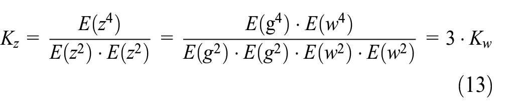
K_{z} = \frac{E (z^{4})}{E (z^{2}) \cdot E (z^{2})} = \frac{E (g^{4}) \cdot E (w^{4})}{E (g^{2}) \cdot E (g^{2}) \cdot E (w^{2}) \cdot E (w^{2})} = 3 \cdot K_{w}

(13)

where, K_w is the kurtosis with mean of AMS w(x), which can be calculated as:

K_{w} = N * \frac{\sum_{i = 1}^{N} w_{i}^{4}}{\sum_{i = 1}^{N} w_{i}^{2} * \sum_{i = 1}^{N} w_{i}^{2}}

(14)

It can be seen from equation (13) that K_z is affected by K_w, which means non-Gaussian road profile with different kurtosis can be synthesized by controlling the kurtosis of AMS.

The PDF of AMS w(x) following a Weibull distribution is:

f (w, λ, k) = {\begin{matrix} \frac{k}{λ} (\frac{w}{λ}) \\ 0 \end{matrix}^{k - 1} \cdot e^{- {(\frac{w}{λ})}^{k}} \begin{matrix} w \geq 0 \\ w < 0 \end{matrix}

(15)

where, k is shape parameter, λ is scaling parameter.

Average of powers of w(x) is:

E (w^{n}) = λ^{n} \cdot Γ (1 + \frac{n}{k})

(16)

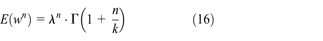
where, Γ is the gamma function.

According to equations (13) and (16), the kurtosis of the non-Gaussian road profile z(x) is:

K_{z} = \frac{E {w^{4}}}{E {w^{2}} \cdot E {w^{2}}} \cdot 3 = \frac{Γ (1 + \frac{4}{k})}{{(Γ (1 + \frac{2}{k}))}^{2}} \cdot 3

(17)

With given kurtosis of non-Gaussian road profile, the shape parameter can be calculated using equation (17).

However, to ensure the high kurtosis of non-Gaussian road profile is correctly transferred to the system response, the frequency content of the AMS must be controlled. A method based on cumulative CDF is used to control the amplitude and frequency of the AMS. The basic idea is to generate a Gaussian AMS with upper frequency limit, which is denoted as Wcut. The AMS is then converted into a Weibull AMS with given parameters, while maintaining the frequency content.

The CDF of Gaussian random signals is:

F_{g} = \frac{1}{2} [1 + \erf (\frac{g}{\sqrt{2}})]

(18)

where, $\erf (g)$ is error function, which defined as:

\erf (g) = \frac{2}{\sqrt{π}} \int_{0}^{g} e^{- t^{2}} dt

(19)

The CDF of a Weibull distribution is:

F_{w} = {\begin{matrix} 1 - e^{- {(x / λ)}^{k}} \\ 0 \end{matrix} \begin{matrix} x \geq 0 \\ x < 0 \end{matrix}

(20)

When λ = 1, the inverse CDF is:

G^{- 1} (y) = {(- \log (1 - y))}^{1 / k}

(21)

According to equations (18) and (21), the Weibull AMS can be calculated as:

w (x) = {(- \log (\frac{1}{2} (1 - \erf (\frac{x}{\sqrt{2}}))))}^{1 / k}

(22)

It should be noted that the AMS needs to be scaled after the CDF transformation. The non-Gaussian road profile can be finally synthesized by using equation (12).

Case study

The golden car has two resonances at 1.17 and 10.1 Hz. In the case study here, the frequency range of the road input spectrum is selected to be 0.5–20 Hz to cover the resonances. The simulated vehicle speed is selected to be 72 km/h, which is a common speed and easy for calculation. f_x is set to 16, which give the sampling frequency for the time signals f_s to be 320 Hz. For the road profile, the standard ISO PSD is used, and the frequency limits 0.5 and 20 Hz corresponds to spatial angular frequencies Ω pi/20 and 2pi, respectively. The road PSD is shown in Figure 8, from which the Gaussian and non-Gaussian road profile are synthesized. The effects of Wcut and kurtosis of road profile on the vehicle response are studied in Section “Effect of Wcut on the FDS of vehicle response” and “Effect of kurtosis of road profile on vehicle response.”

Figure 8.

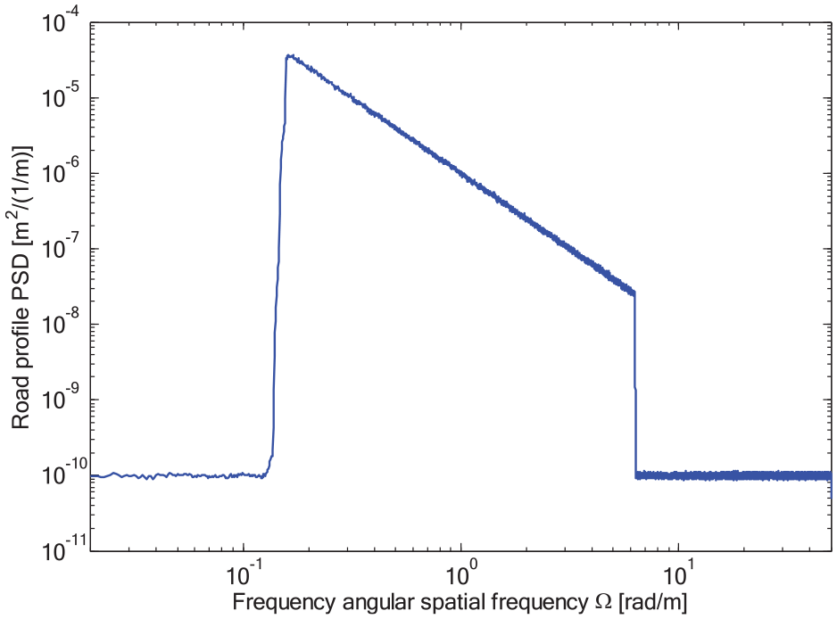
PSD in spatial angular frequency domain.

Effect of Wcut on the FDS of vehicle response

A Gaussian road profile was synthesized from PSD in Figure 8. The first 3 km profile is shown in Figure 9. With a given kurtosis of 8, five non-Gaussian road profiles with the same PSD and different Wcut ([0.01 0.1 0.5 1 10]) were synthesized. To keep it simple, only the results with Wcut = 0.01 and 0.5 rad/m were shown here. The first 3 km profiles and corresponding AMS are shown in Figures 10 and 11. From Figures 10 and 11 we can see that a low Wcut should be selected so that the AMS and synthesized non-Gaussian profile is slowly varying.

Figure 9.

Synthesized Gaussian road profile.

Figure 10.

Synthesized profile with Wcut = 0.01: (a) non-Gaussian road profile and (b) corresponding AMS.

Figure 11.

Synthesized profile with Wcut = 0.5: (a) non-Gaussian road profile and (b) corresponding AMS.

The effect of Wcut on FDS of vehicle response is shown in Figure 12. As can be observed in Figure 12, a bigger Wcut results in a lower FDS over the entire frequency range. The deviation between the FDS with bigger Wcut and the FDS under Gaussian road profile is smaller, due to the fact that the kurtosis of the vehicle response is smaller with bigger Wcut.

Figure 12.

FDS of vehicle response under Gaussian and non-Gaussian road profile.

Effect of kurtosis of road profile on vehicle response

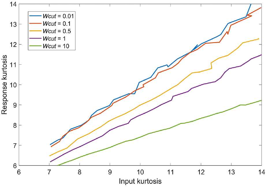
With different Wcut, the kurtosis of vehicle response under road profile excitation with different kurtosis (from 7 to 14 with a stepping value of 0.25) is shown in Figure 13. From Figure 13 we can observe that as Wcut increases, the response kurtosis decreases. A low Wcut should be selected so that the high input kurtosis is correctly transferred to the vehicle response, that is, the kurtosis of vehicle response is almost the same as the kurtosis of road profile excitation.

Figure 13.

Response kurtosis with different input kurtosis.

The FDS of vehicle response under road profile excitation with different input kurtosis, including Gaussian road profile, is shown in Figures 14 and 15, with Wcut = 0.01 rad/m and Wcut = 10 rad/m.

Figure 14.

FDS of vehicle response under road profile excitation (Wcut = 0.01).

Figure 15.

FDS of vehicle response under road profile excitation (Wcut = 10).

From Figure 14 we can see that with a low Wcut, the FDS of vehicle response increases over the entire frequency range as the kurtosis of road profile increases. However, from Figure 15 we can see that, as Wcut increases, the FDS of the vehicle response only increases over the high frequency range. For the low frequency range, the FDS with kurtosis 7 and 11 are basically the same as that with kurtosis 3. The reason for that is, as Wcut increases, the AMS is not slowly varying anymore. The high kurtosis of synthesized non-Gaussian road profile is not correctly transferred to the vehicle response, which also justifies the result of Figure 13.

Conclusion

Gaussian road profile is widely used to study vehicle response and fatigue damage potential, while the measured road profile is often non-Gaussian. The vehicle response under Gaussian and non-Gaussian road profile excitation is investigated in this paper. A new amplitude modulation method which has full control of cutoff frequency and amplitude of the amplitude modulation signal is presented to synthesize non-Gaussian road profile with different kurtosis. The forced response of a quarter vehicle under non-Gaussian road profile excitation is then calculated using the ramp invariant digital filter method. The kurtosis and FDS of the vehicle response are compared under road profile excitation with different kurtosis and cutoff frequency. The results show that, a small cutoff frequency (e.g. 0.01 rad/m in the case study) should be selected so that the high kurtosis (from 7 to 14 with a stepping value of 0.25 in the case study) of the non-Gaussian road profile is correctly transferred to the vehicle response, and the kurtosis of vehicle response is the same as that of the input road profile. The FDS of the vehicle response increases over the entire frequency range as the kurtosis of the input road profile increases, which lays the foundation for a more accurate and effective fatigue test.

Footnotes

Handling Editor: Chenhui Liang

Author contributions

Conceptualization, F.X., H.Y., and K.A.; methodology, F.X. and H.Y.; software, F.X.; validation, F.X., H.Y., and K.A.; formal analysis, H.Y.; investigation, F.X. and K.A.; resources, F.X. and K.A.; data curation, F.X., H.X., and K.A.; writing – original draft preparation, H.Y.; writing – review and editing, H.Y.; visualization, F.X.; supervision, F.X.; project administration, F.X.; funding acquisition, F.X. All authors have read and agreed to the published version of the manuscript.

Declaration of conflicting interests

The author(s) declared no potential conflicts of interest with respect to the research, authorship, and/or publication of this article.

Funding

The author(s) disclosed receipt of the following financial support for the research, authorship, and/or publication of this article: This study was supported by The National Natural Science Foundation of China (Grant # 52102443).

ORCID iD

Fei Xu

Data availability

The data used to support the findings of this study are available from the corresponding author upon request.

References

ISO 8608. Mechanical vibration - road surface profiles - reporting of measured data, ISO 8608:2016. International Organization for Standardization, ISO, 2016.

Hui

Kawai

, et al. Non-stationary and non-Gaussian characteristics of wind speeds. Wind Struct 2017; 24: 59–78.

Decker

Savaidis

Measurement and analysis of wheel loads for design and fatigue evaluation of vehicle chassis components. Fatigue Fract Eng Mater Struct 2002; 25: 1103–1119.

Steinwolf

Cornelis

Peeters

, et al. On the use of kurtosis control methods in shaker testing for fatigue damage. J Test Eval 2020; 48: 538–556.

Steinwolf

Peeters

Auweraer

. Two methods of generating random excitations with increased kurtosis for in-house testing of vehicle components. In: 22nd international congress on sound and vibration, Florence, Italy, 2015.

Zheng

Guoping

Huaihai

. Stationary non-Gaussian random vibration control: a review. Chin J Aeronaut 2021; 34: 350–363.

Smallwood

. Vibration with non-Gaussian noise. J IEST 2009; 52: 13–30.

Cui

Geng

Wang

, et al. Study of the amplitude modulation method for kurtosis control purposes. Mech Syst Signal Process 2022; 179: 109399.

Jiang

, et al. Synthesis of running RMS-induced non-Gaussian random vibration based on Weibull distribution. J Vibroengineering 2015; 17: 3662–3674.

10.

Jiang

. On the shaker simulation of wind-induced non-Gaussian random vibration. J Shock Vib 2016; 2016: 5450865.

11.

Yang

Zhu

Gao

, et al. Fatigue life analysis of vehicle systems under non-Gaussian excitation. Int J Automot Mech Eng 2020; 17: 7956–7966.

12.

Lei

Jiang

Zeng

, et al. Research on the transmission law of kurtosis of SDOF system under nonstationary and non-Gaussian random excitations. Mech Syst Signal Process 2022; 165: 108292.

13.

Tao

Cheng

. Dynamic stress response and fatigue life of cantilever beam under non-Gaussian base excitation. J Vibroengineering 2014; 16: 1284–1296.

14.

Kihm

Rizzi

Ferguson

, et al. Understanding how kurtosis is transferred from input acceleration to stress response and it’s influence on fatigue life. In: 11th international conference on recent advances in structural dynamics, Pisa, Italy, 1–3 July 2013, pp.1–16.

15.

Hosoyama

Tsuda

Horiguchi

. Development and validation of kurtosis response spectrum analysis for antivibration packaging design taking into consideration kurtosis. Packaging Technol Sci 2020; 33: 51–64.

16.

Louhghalam

Tootkaboni

Ulm

. Roughness-induced vehicle energy dissipation: statistical analysis and scaling. J Eng Mech 2015; 141: 04015046.

17.

ISO 18431-4:2007. Mechanical vibration and shock - signal processing - part 4: shock-response spectrum analysis, ISO 18431-4:2007. International Organization for Standardization, ISO, 2007.

18.

Henderson

Piersol

. Fatigue damage related descriptor for random vibration test environments. J Sound Vib 1995; 29: 20–25.

19.

Angeli

Cornelis

Troncossi

. Synthesis of Sine-on-Random vibration profiles for accelerated life tests based on fatigue damage spectrum equivalence. Mech Syst Signal Process 2018; 103: 340–351.

On vehicle response under non-Gaussian road profile excitation

Abstract

Keywords

Introduction

Theoretical background

Gaussian and non-Gaussian road profile

Vehicle model

Fatigue damage spectrum (FDS)

Synthesis of non-Gaussian road profile

Case study

Effect of Wcut on the FDS of vehicle response

Effect of kurtosis of road profile on vehicle response

Conclusion

Footnotes

Author contributions

Declaration of conflicting interests

Funding

ORCID iD

Data availability

References