Bayesian neural networks for uncertainty quantification in remaining useful life prediction of systems with sensor monitoring

Abstract

Many machine learning (ML) algorithms have been developed over the past two decades for prognostics and health management (PHM) of complex engineering systems. However, most of the existing algorithms tend to produce point estimates of a variable of interest, for example the equipment’s remaining useful life (RUL). The point estimation of the RUL often neglects the uncertainty inherent in model parameters and/or the uncertainty associated with data inputs. Bayesian Neural Networks (BNNs) have shown a lot of promise in obtaining credible intervals for model parameters, thus accounting for the uncertainties inherent in both the model and data. This paper proposes a deep BNN model with the Monte Carlo (MC) dropout method to predict the RUL of engineering systems equipped with sensors and monitoring instruments. The model is tested on NASA’s Turbofan Engine Degradation Simulation Dataset and the results are discussed and analyzed. It is revealed that the method can produce highly accurate predictions for RUL distribution parameters in safety critical components.

Introduction

Prognostics and health management (PHM) is a field of research and application which aims to maintain the reliable, efficient, economic, and safe operation of engineering equipment, systems, and structures. It involves the process of data acquisition, diagnostics, health state estimation, prognostics, and maintenance decision-making. ¹ The penultimate activity in this process, that is, prognostics, primarily involves predicting the remaining useful life (RUL) of systems or components. RUL is defined as the time left before the degradation of an equipment exceeds a failure threshold. ² In other words, RUL is the time from the detection of an incipient failure to the time when the system performance crosses a failure threshold. An important point to note is that the RUL could be measured based on various criteria, such as calendar time (e.g. days, weeks, and months), number of charge and discharge cycles (e.g. for a battery), number of fatigue cycles (e.g. for a steel bridge structure), or even in terms of usage, examples of which include flight hours for aircraft engines, runtime for machines, or mileage for automobiles.

Over the past two decades, many researchers have had to contend with different challenges encountered in the process of predicting RUL. Some of these key challenges have been discussed in Engel et al. ³ The paper explored the necessary conditions to achieve the desired convergence between the accuracy of prediction and the uncertainty in RUL, as the system continues to degrade. RUL predictions derived in the paper were presented by probability distributions to capture the uncertainty in features (i.e. data) as well as in prediction model. Despite many follow-up studies in PHM research field and even with a myriad of many new approaches being adopted in the era of Big Data, some core challenges with uncertainty quantification of RUL prediction remain yet to be solved.

The RUL prediction methods in literature can be broadly classified into two types: physics-based and data-driven. Physics-based methods apply theoretical mathematical models to interpret degradation processes over time or cycles. These models are usually expressed in terms of differential equations which can be solved using either analytic or numerical methods, depending on the level of complexity of the problem. Deriving a mathematical equation for the evaluation of degradation process for complex systems and in rapidly changing environments is sometimes impossible or infeasible. As such, data-driven approaches have become more prominent in the PHM field as they rely on system test data to identify the characteristics of damage state and predict the RUL without relying on any physical model.

Given the present proliferation of advanced sensor technologies, data storage capabilities, and increased computing resources, the use of artificial intelligence (AI) techniques as a data-driven technology in understating the underlying failure signatures for the purpose of predicting RUL has attracted widespread attention. AI-driven RUL models prove to be accurate and remarkably efficient. However, most of the algorithms proposed up to now produce point estimates of RUL,^4–6 with accuracies measured in terms of the error between the point estimate and the true RUL value which, in reality, is unknown. In addition, the sensor data may be inherently noisy, resulting in another layer of uncertainty known as “aleatoric” uncertainty. Moreover, the use of AI algorithms involves the tuning of different hyperparameters such as the number of layers of a neural network, the regularization parameter, the number of neurons in each layer or even the type of AI algorithm used; all these are variabilities that introduce uncertainty in the prognostic process itself and this class of uncertainty is termed as “epistemic” uncertainty.

In an attempt to overcome some of the aforementioned limitations associated with uncertainty quantification in RUL prediction, researchers have developed many new techniques, among which the most common are “Bayesian” approaches. Particle filter-based algorithms^7–9 and Kalman filter-based algorithms,^10–12 which are both based on Bayesian techniques, have been adopted for RUL prediction. However, in strict technical terms, these methods are essentially approaches for health state estimation as they make use of past data to predict the present health state of a system and then based on the present health state and additional data, predict future health states. ¹³ The RUL is thereby obtained by deduction, inferring RUL from the time it will take for a system to get into a failed state. Other researchers have used Dynamic Bayesian Networks (DBNs) and Hidden Markov Models (HMMs) to address uncertainty in prognostics.^14–16 Gaussian Process Regression (GPR) is also a Bayesian technique that has been used extensively by researchers to quantify the uncertainty in terms of variance for RUL predictions, in particular for cases where the data is sparse.^17–19 Deutsch and He ²⁰ employed a resampling technique to address the fact that RUL is not deterministic. They used deep learning algorithms to make several repeated RUL predictions by removing one instance of the training data during each prediction and updating the RUL values progressively, thereby obtaining the RUL distribution parameters. Liu et al. ²¹ also used an adaptive recurrent neural network (ARNN) to predict the RUL values by making 50 prediction runs and obtained the RUL distribution parameters. The drawback of the model was that the uncertainties in the model and data were not implicitly addressed. As regards AI algorithms, a key step in the process involves preprocessing of data, which includes smoothing the data to remove noise, discarding outliers, and even generating entirely new features via feature crosses that involves some mathematical transformation of the original sensor data. Feature crosses produce additional features that are meant to be more informative for prognostics purposes. While these approaches are aimed at handling some aspects of aleatoric uncertainty (i.e. uncertainty in sensor data), data preprocessing itself is somewhat subjective and injects its own layer of uncertainty.

Among many Bayesian techniques within the sphere of AI algorithms used for prognostics, the Bayesian Neural Networks (BNNs) are one of the most popular approaches to uncertainty quantification. As expounded in the work of Gal ²² and following foundational studies in BNN,^23–27 additional efforts in solving the problem of approximating the posterior distribution of model weights (as a fundamental problem in BNN) can be found in the works of Barber and Bishop, ²⁸ Minka, ²⁹ and Graves ³⁰ However, most of those early approaches suffered from the drawbacks of scalability to larger data, adaptability to complex models, and ease of use by non-core practitioners. ²² Recent advances as presented in other studies^31–34 have helped to address some of these challenges. As such, computer scientists and AI practitioners within the PHM domain have recently started adopting BNNs in uncertainty quantification. Peng et al. ³⁵ proposed a Bayesian deep learning method to address the issue of model (or epistemic) uncertainty. Kim and Liu ³⁶ and Li et al. ³⁷ implemented Bayesian deep learning algorithms for RUL prediction by incorporating both epistemic and aleatoric uncertainties. However, all attempts in the literature using BNNs are analytically cumbersome and overly theoretical, which may be a turn-off for the core engineers for which these methodologies should be useful in a practical way. Apart from the theoretically rigorous presentation, the existing approaches assume that the prior distribution of the predicted RUL is a normal distribution. However, in reality, the true distribution of the RUL is unknown and may not be necessarily normal.

In view of the above-mentioned gaps in the literature, the current study aims to propose a deep BNN algorithm with the Monte Carlo (MC) dropout approach to derive the mean RUL prediction as well as a credible interval without making any explicit assumptions about the true RUL distributions. Thus, an approximation of the RUL distribution is made which is as close to the true RUL distribution as possible. Another specific contribution of this study is that our proposed algorithm takes both aleatoric and epistemic uncertainties into account. This fills the gap in earlier heuristic approaches that only attempt to achieve uncertainty quantification by making several, repeated point estimations of the RUL, thereby only indirectly accounting for epistemic uncertainty and not accounting for aleatoric uncertainty. In addition, another specific contribution of this research is the achievement of results that are very amenable to use in real-life systems since the uncertainties are quantified in numerical terms rather than qualitatively, thus providing interpretable information for use in maintenance planning and end-of-life management.

The remaining part of this paper is organized as follows. Section 2 provides a detailed perspective of uncertainty quantification approaches in PHM. Section 3 proposes the Monte Carlo dropout BNN algorithm used for RUL prediction in this study. Section 4 presents and discusses the results of testing the proposed algorithm on NASA’s Turbofan engine degradation dataset (CMAPSS). Section 5 presents the conclusion and highlights areas of future work.

Uncertainty quantification in PHM

Methods of incorporating uncertainty in RUL prediction are either testing-based (which rely on offline data collected from accelerated life testing) or condition-based (which rely on online data provided from condition monitoring devices).^13,38 Testing-based methods are often applied to inexpensive components, several of which can be run until failure to obtain lifetime data and failure probability distributions while condition-based methods are applied to complex systems. In what follows, different types of uncertainties in the PHM domain are reviewed.

Types of uncertainties

Conventionally, uncertainties have been categorized as aleatoric (in relation to data) and epistemic (in relation to model parameters). However, Sankararaman ¹³ argues that a more bespoke categorization is necessary for prognostics and RUL prediction. Thereafter, Sankararaman and Goebel ³⁸ suggested four categories of uncertainty, namely:

• Present uncertainty: This is the uncertainty inherent in the estimation of the present health state, which, in PHM, is a necessary step before predicting RUL. The sources of this uncertainty include sensor noise, gain and bias, data pre-processing tools and techniques, and filtering and estimation techniques. This uncertainty is analogous to aleatoric uncertainty in conventional categorizations.

• Future uncertainty: This corresponds to the inherent uncertainty in predicting future health conditions. Sources of this uncertainty include future loading, environmental conditions, and operating scenarios.

• Modeling uncertainty: This uncertainty is due to the fundamental difference between the true system output and the output represented by the chosen or derived model. This uncertainty manifests itself (whether by a linear, polynomial, or a more complicated relationship captured via a neural network) in the model or the model parameters.

• Prediction method uncertainty: This refers to the way that present, future, and modeling uncertainties are combined to influence the RUL estimates, with its associated uncertainty. With the same dataset and under the same conditions, different prognostics models may yield different RUL values. In fact, even the same method may yield different RUL values for repeated runs of the algorithm due to variation in initial sampling (leading to sampling errors) and different approaches used in approximating the model parameters. This therefore will underscore the fact that although the true RUL value may be deterministic, the results from a data-driven prediction algorithm are random variables. Both the modeling and prediction method uncertainties are analogous to epistemic uncertainty.

Approaches to uncertainty quantification

Several approaches have been proposed by PHM researchers for uncertainty quantification in RUL prediction. A brief overview of the most popular approaches is given below:

• “Classical” methods: Traditionally, failure probability data for a component are obtained by running the component until failure. This produces a sample from which failure probability distribution parameters can be estimated. The population failure probability distribution parameters are then inferred from the sample parameters using statistical techniques. The main limitation of this approach is its impracticality for complex systems.

• Data preprocessing: Sensor data comes with noise, signal gain and bias. This causes a major source of uncertainty. To address this issue, some data preprocessing techniques such as smoothing, filtering and outlier removal or replacement can be employed.^39,40 Although these approaches generally tend to make the resulting data or features more informative, their impact, in quantitative terms, on reducing the inherent uncertainty is not yet well understood.

• Several runs of point estimates: One way some researchers have attempted to quantify uncertainty is by making several repeated point estimates of RUL using a model or an algorithm, thereby generating a sample of RUL values with enough statistical significance and then estimating the population parameters based on the sample observations. Deutsch and He ²⁰ used a resampling technique by eliminating one training data for each run of their deep learning-based algorithm and iterated this until the entire training data was covered, obtaining several point estimates of RUL as well as its distribution parameters. Liu et al. ²¹ used a similar approach to predict the RUL distribution parameters. However, their heuristic approach failed to directly account for the uncertainty in the data or in the model.

• Bayesian techniques: The methods employing Bayesian techniques for health state estimation and RUL prediction include particle filtering,^7–9 Kalman filtering and its variants,^10–12 HMMs,^41–43 and DBNs.^15,16 These methods predict the system’s health state based on available data and then employ recursive or sequential techniques to update the health state as additional data become available, using the time steps up till the time when the system health state reaches a failure threshold. The time steps or slices are then used as basis for calculating the RUL. Even though these are fundamental approaches being used to estimate the system’s health state, ¹³ they provide probability distributions for the RUL, thus accounting for uncertainty. Some of these techniques have also been combined with classical reliability methods to achieve more accuracy in RUL prediction. Bressel et al. ⁴⁴ used an extended Kalman filter to estimate the state of health and the dynamics of degradation in a Proton Exchange Membrane Fuel Cell (PEMFC) under variable loading. An inverse First Order Reliability Method (iFORM) using limit state functions was formulated to predict the RUL by extrapolating the state of health until a failure threshold is reached, giving the RUL along with a 90% confidence interval.

Another common approach involves the use of a model to predict RUL and the subsequent use of Bayesian inference to update the RUL values and its distribution parameters as more data becomes available. Zhao et al. ⁴⁵ integrated condition monitoring data to update the parameters of their model-based RUL prediction methodology using Bayesian inference, thereby updating the RUL and the associated uncertainty as more data became available. An et al. ⁴⁶ also used Bayesian inference as a statistical method to address uncertainty in terms of noise in data (i.e. aleatory uncertainty) and model weights (i.e. epistemic uncertainty). The authors compared their method with the method of using repeated predictions of RUL to obtain its distribution. The method was found to outperform the repetition method in cases where there is large noise in data, or the degradation mechanisms are complex. Gao et al. ⁴⁷ proposed a joint prognostic model that uses a Maximum Likelihood Estimate (MLE) at an offline stage to determine the prior distribution for each input signal, after which the distribution parameters obtained using MLE method are fed, as inputs, into a three-layer neural network to predict the degradation. During a subsequent online stage, Bayesian updating is used, along with real-life sensor data collected from the unit whose RUL is to be predicted, to obtain the posterior distribution of the parameters in the degradation model, thus obtaining an updated RUL distribution. Liu et al. ⁴⁸ proposed an RUL prediction method based on an exponential stochastic degradation model that considered multiple uncertainty sources simultaneously, while using a Bayesian-Extreme Learning Machine to further quantify the uncertainties and predict the RUL of crystal oscillators.

The advantage of BNN models over other approaches is that uncertainty quantification is implicitly modeled in the design of the network such that BNN models directly generate RUL values as probability distributions rather than generating repeated point estimates of the RUL. Peng et al. ³⁵ incorporated uncertainties into prognostics by using Bayesian deep-learning-based models. A Bayesian multi-scale convolutional neural network was proposed to predict the RUL with confidence interval bounds for bearings while a Bayesian bidirectional long short-term memory (LSTM) algorithm was used to predict the RUL for turbofan engines. For both models, variational inference (VI) was used to approximate the posterior distribution of the model parameters, given the training data and the training RUL values. A limitation of the study was that the authors only considered the uncertainty in model parameters. In an attempt to close this gap, Li et al. ³⁷ developed a Bayesian deep learning framework for RUL prediction by incorporating the epistemic and aleatoric uncertainties. The framework, which was tested on a dataset from high voltage circuit breakers, was implemented using a gated recurrent unit (GRU), which is a form of the LSTM algorithm. While addressing the uncertainty in data as well as in model parameters, a sequential Bayesian boosting framework was incorporated within the algorithm to help sequentially shrink the predicted credible interval. This final step, fundamentally, is similar to the study by Deutsch and He ²⁰ where several RUL predictions were made and then fitted onto a distribution to account for uncertainties. The approach of using BNN and breaking down the prognostics process into two or more steps has also been studied by other researchers. Kim and Liu ³⁶ proposed a Bayesian deep neural network for the prediction of RUL and quantification of uncertainties. The authors considered two groups of uncertainty, including weight uncertainty (which accounts for the uncertainty in model weights) and degradation uncertainty (which accounts for the combined effects of signal/sensor measurement errors and variability from one system to another. The model was formulated in two parts: one part was a Bayesian LSTM which was used to predict the RUL while accounting for uncertainty in model weights, and the second part was a feed forward neural network (FFNN) which takes RUL estimates as input and establishes a monotonic relationship between the RUL and degradation uncertainty in terms of the variance of the data. The weights of the FFNN were implicitly modeled within the Bayesian LSTM framework. Kraus and Feuerriegel ⁴⁹ proposed a structured-effect neural network (SENN) model to address the issue of interpretability of machine learning (ML) approaches in RUL prediction. The SENN algorithm included three components; the first component was a non-parametric part with probabilistic lifetime models fitted with Weibull or lognormal distributions; the second component was a linear regression model using current condition data, while the third component uses an LSTM to model non-linearities in the data using variational Bayesian inference to estimate the model parameters.

Aside the goal of quantifying uncertainties, other researchers have also used BNN as an important algorithm in the scenario of small and noisy data as BNNs tend to be more robust to overfitting. Vega and Todd ⁵⁰ used BNNs to estimate the RUL for structures equipped with structural health monitoring (SHM) systems, where minimal data was obtained from a finite element analysis (FEA) model which mimicked real-life inspection data obtained from miter gates. The cost implication of using prognostics as compared to conventional inspection methods was also evaluated using the probability confidence bounds estimated by BNNs. Guo et al. ⁵¹ estimated RUL for an external gear pump using a Radial Basis Function with Bayesian regularization, which is a Bayesian approach toward minimizing overfitting during the training process. Xiao et al. ⁵² used a self-attention-based adaptive mechanism to construct health indicators in electronics application for insulated gate bipolar transistor (IGBT) and then used MC dropout as a BNN approach for RUL prediction for the IGBT. Li and He ⁵³ also proposed a deep convolutional neural network (DCNN) combined with Bayesian optimization and adaptive batch normalization (AdaBN) for RUL prediction. The method yielded a self-optimized network structure and hyperparameters selection (such as number of neural network layers, learning rate, batch size, etc.) as against random search and grid search. However, the algorithms in both the studies of Guo et al. ⁵¹ and Li and He ⁵³ generated point estimates for the RUL, rather than probability distributions. Gaussian Process Regression (GPR) is also a Bayesian technique that provides uncertainty quantification in terms of variance for RUL predictions and has been used extensively by researchers because it is also particularly well suited to scenarios with sparse data.^17–19 Other Bayesian techniques that have been used for uncertainty quantification in RUL prediction include Dempster-Shafer theory and Bayesian Monte-Carlo methods ⁵⁴ and the Relevance Vector Machine.^55,56

For systems that experience multiple failure modes, the study by Gandur and Ekwaro-Osir ⁵⁷ used BNNs to predict the RUL for bearing data as well as for a battery degradation problem and showed that the uncertainty increases with increase in the number of failure modes. The findings are important for applications in complex systems, and it would be useful to investigate further to find which failure modes contribute more to increase in uncertainty. Another recent area of machine learning-based RUL prediction research is in attention-based networks. Attention networks utilize attention mechanisms to emphasize task-relevant information in deep learning networks through enhanced adaptive feature representation. To incorporate uncertainty quantification, Wang et al. ⁵⁸ used a Bayesian Kernel attention network for RUL prediction in bearings. The method produced more interpretable and trustworthy results in terms of the credible intervals for the RUL, along with the mean RUL prediction, thus providing a lot more information for decision-making when compared to existing methods of implementing attention networks that ignore uncertainty information and thus lead to overconfident RUL predictions. The multifarious collection of Bayesian methods used for uncertainty quantification in prognostics demonstrates the fact that it is a challenge of huge significance in the context of using RUL predictions as a basis for maintenance decision-making.

BNN algorithm for RUL prediction

In this section, a concise background of BNNs is presented, along with our proposed BNN algorithm for RUL prediction under uncertainty.

BNN background

To get a full picture of the RUL prediction algorithm proposed in this work, a brief background of BNNs is provide below:

• (i) Bayes’ theorem: Let $p\left(\mathcal{D}\right)$ denote the marginal or unconditional probability of observing a dataset, $\mathcal{D}$ , irrespective of all other occurrences. Also, let $p\left(\omega \right)$ denote the marginal or unconditional probability of observing a set of neural network weights, $\omega$ , irrespective of the data or other parameters. The joint probability of these two observations is denoted by $p(\omega ,\mathcal{D})$ while the conditional probability of one observation, given another observation, is denoted by $p(\omega |\mathcal{D})$ , which, in this case, stands for the probability of observing the network weights, $\omega$ , given the dataset, $\mathcal{D}$ . Bayes’ theorem connects all these probabilities as given in equation (1):

$$p(\omega |\mathcal{D})=\frac{p(\omega ,\mathcal{D})}{p\left(\mathcal{D}\right)},$$

(1)

where $p(\omega ,\mathcal{D})$ represents the joint probability between the model weights and the observed data, given in equation (2) as:

$$p(\omega ,\mathcal{D})=p(\mathcal{D}|\omega )p\left(\omega \right).$$

(2)

The application of Bayes’ theorem to neural networks involves having a prior belief about the model weights, which corresponds to weight initialization in traditional deep learning. This prior belief is denoted by $\mathit{p}\left(\mathbf{\omega }\right)$ . The marginal probability of observing the data, $\mathit{p}\left(\mathcal{D}\right)$ , is referred to as the evidence. The probability of observing the model weights given that the data (or evidence) has been observed (typically obtainable after training the model) represents the posterior probability denoted by $\mathit{p}(\mathbf{\omega }|\mathcal{D})$ . The inverse of the posterior, $\mathit{p}(\mathcal{D}|\mathbf{\omega })$ , represents the likelihood that the data or evidence, $\mathcal{D}$ , will be observed, given a set of weights, $\mathbf{\omega }$ . Therefore, Bayes’ theorem can be expressed as given in equation (3):

$$\mathrm{Posterior}=\frac{\mathrm{Likelihood}\times \mathrm{Prior}}{\mathrm{Evidence}}.$$

(3)

• (ii) Probabilistic models: The prediction of RUL is inherently a regression problem. The core task of a neural network developed for a regression task is to make predictions given a training dataset, $\mathcal{D}$ , which contains $n$ input-output pairs of the form $\mathcal{D}=\{x_1,y_1;x_2,y_2;\dots ;x_n,y_n\}$ . A neural network can be formulated as a probabilistic model as $p(y|x,\omega )$ . The joint distribution between the model weights and the data, $p(\omega ,\mathcal{D})$ , even before training, can be defined using the prior belief, $p\left(\omega \right)$ , and the choice of the model (or likelihood), $p(\mathcal{D}|\omega )$ , using equation (2). The likelihood is determined by the model architecture and the choice of the loss function used to achieve the optimization objective. For a conventional regression problem with a known variance and the loss measured as the mean squared error (MSE), the mean of a Gaussian likelihood can be specified by the network output as given in equation (4) ⁵⁹ :

$$p(\mathcal{D}|\omega )=p(y|x,\omega ).$$

(4)

Typically, all the samples in the dataset, $\mathcal{D}$ , are assumed to be independent and identically distributed, and the likelihood can be written as a product of the contribution from all the $\mathit{n}$ individual samples in the dataset, given in equation (5) as:

$$p(\mathcal{D}|\omega )=\underset{i=1}{\overset{n}{\Pi }}p(y_i|x_i,\omega ).$$

(5)

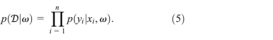
It can be shown that maximizing the likelihood given in equation (5) yields the Maximum Likelihood Estimate (MLE) of the model weights, $\mathbf{\omega }$ , with the negative log likelihood as the optimization objective during training. However, the MLE produces point estimates and is prone to overfitting as the regularization terms are all discarded. ⁶⁰ Further, the full form of equation (1) can be written as given in equation (6):

$$p(\omega |\mathcal{D})=\frac{p(\mathcal{D}|\omega )p\left(\omega \right)}{p\left(\mathcal{D}\right)}.$$

(6)

In practice, during the training process, the training data or evidence is constant, so the term $\mathit{p}\left(\mathcal{D}\right)$ in equation (6) normalizes the likelihood, making it a proper probability distribution. Therefore, equation (6) is reducible to:

$$p(\omega |\mathcal{D})\propto p(\mathcal{D}|\omega )p\left(\omega \right),$$

(7)

or in another words, Posterior $\propto$ Likelihood $\times$ Prior. From equation (7), it is clear that maximizing $p(\mathcal{D}|\omega )\mathrm{p}\left(\omega \right)$ corresponds to the Maximum A Posteriori (MAP) estimate, with the same optimization objective as with the MLE, that is, the negative log likelihood. The MAP, however, includes a regularization term but still yields a point estimate similar to the MLE. ⁶⁰ So, the MLE and the MAP, though being probabilistic models for the neural network outputs, only yield point estimates and do not account for uncertainty.

• (iii) Variational inference: Suppose that we have full probability distributions over the parameters of the neural network, then uncertainties can be considered. To model this, the output, $y$ , will be a continuous variable and not a fixed value or point estimate, with its distribution conditional upon an input, $x$ , for which prediction is to be made, and the training data, $\mathcal{D}$ . The output or posterior predictive distribution, $p(y|x,\mathcal{D})$ , is usually calculated by combining (i.e. integrating) the individual predictive contributions from a given, finite set of distributions of model weights (i.e. $p(y|x,\omega )$ ), and weighing each prediction with its posterior probability, $p(\omega |\mathcal{D})$ . As presented in Gal and Ghahramani ⁶¹ and Duerr et al. ⁶² this integral is given as in equation (8) below:

$$p(y|x,\mathcal{D})=\int p(y|x,\omega )p(\omega |\mathcal{D})d\omega .$$

(8)

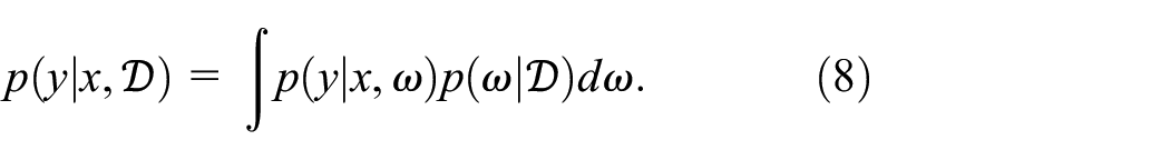
It is a known problem that the analytical solution to the posterior predictive distribution, $\mathit{p}(\mathbf{\omega }|\mathcal{D})$ , in equation (8) is intractable. Common approaches used to overcome this problem in BNNs is via variational inference (VI) and MC dropout. With VI, the analytically intractable posterior, $\mathit{p}(\mathbf{\omega }|\mathcal{D})$ , is approximated using a posterior, ${\mathit{q}}_{\mathbf{\theta }}\left(\mathbf{\omega }\right)$ , whose analytical form is known, with a set of parameters, $\mathbf{\theta }$ . The usual assumption for ${\mathit{q}}_{\mathbf{\theta }}\left(\mathbf{\omega }\right)$ , which is called the variational distribution, is a standard normal distribution. As shown by Barber and Bishop, ²⁸ the variational distribution, ${\mathit{q}}_{\mathbf{\theta }}\left(\mathbf{\omega }\right)$ , can be used to approximate the true posterior distribution, $\mathit{p}(\mathbf{\omega }|\mathcal{D})$ , by minimizing the Kullback-Leibler (KL) divergence between ${\mathit{q}}_{\mathbf{\theta }}\left(\mathbf{\omega }\right)$ and $\mathit{p}(\mathbf{\omega }|\mathcal{D})$ . The KL divergence between both distributions is defined by equation (9) as:

$$\mathrm{KL}(q_{\theta }\left(\omega \right)\parallel p(\omega |\mathcal{D}))=\int q_{\theta }\left(\omega \right)\log \frac{q_{\theta }\left(\omega \right)}{p(\omega |\mathcal{D})}d\omega .$$

(9)

The KL divergence, as in Barber and Bishop, ²⁸ Gandur and Ekwaro-Osir, ⁵⁷ Duerr et al. ⁶² can be reduced to equation (10) as given below:

$$\begin{array}{c}\multicolumn{1}{c}{\mathrm{KL}(q_{\theta }\left(\omega \right)\parallel p(\omega |\mathcal{D}))={\mathbb{E}}_q[\log \frac{q_{\theta }\left(\omega \right)}{p\left(\omega \right)}-\log p(\mathcal{D}|\omega )]}\\ +\log p\left(\mathcal{D}\right).\hfill \end{array}$$

(10)

Equation (10) can be further reduced to equation (11) as given below:

$$\mathrm{KL}(q_{\theta }\left(\omega \right)\parallel p(\omega |\mathcal{D}))=-\mathcal{F}\left(q_{\theta }\right)+\log p\left(\mathcal{D}\right),$$

(11)

where $\mathcal{F}\left({\mathit{q}}_{\mathbf{\theta }}\right)$ is the eventual optimization objective and given in equation (12) as in Goan and Fookes ⁵⁹ :

$$\mathcal{F}\left(q_{\theta }\right)={\mathbb{E}}_q\left[\log p(\mathcal{D}|\omega )\right]-\mathrm{KL}(q_{\theta }\left(\omega \right)\parallel p\left(\omega \right)).$$

(12)

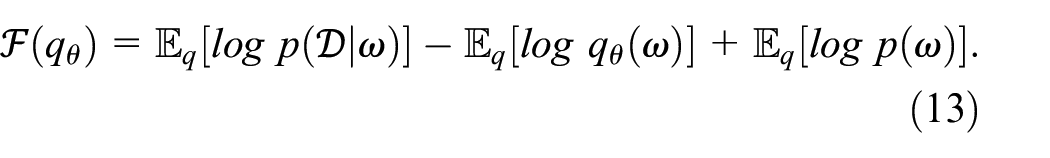
The first term in equation (12) represents the expected value of the log likelihood with respect to the variational distribution parameters and the second term represents the KL divergence between the variational and the prior distribution. The relationship described in equation (11) can be visualized as shown in Figure 1.

Figure 1.

The KL divergence between true and approximate posteriors is equal to evidence lower bound (ELBO) (adapted from Barber and Bishop ²⁸ and Gandur and Ekwaro-Osir ⁵⁷ ).

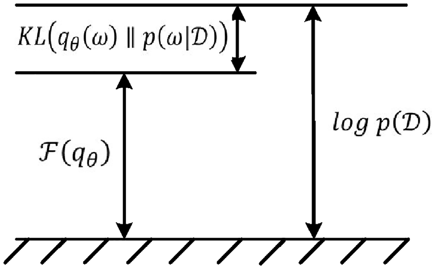
It can be seen from Figure 1 that by minimizing the KL divergence, $\mathcal{F}\left({\mathit{q}}_{\mathbf{\theta }}\right)$ is maximized and approaches the logarithm of the marginal likelihood (i.e. logarithm of the evidence). Hence, $\mathcal{F}\left({\mathit{q}}_{\mathbf{\theta }}\right)$ is commonly referred to as the Evidence Lower Bound (ELBO). So, minimizing KL divergence is equivalent to maximizing the ELBO. During optimization using backpropagation, only the terms containing the variational parameters remain, as all other terms reduce to zero. Equation (12) can be expanded, as shown in Blundell et al., ³³ to obtain equation (13) as given by:

$$\mathcal{F}\left(q_{\theta }\right)={\mathbb{E}}_q\left[\log p(\mathcal{D}|\omega )\right]-{\mathbb{E}}_q\left[\log q_{\theta }\left(\omega \right)\right]+{\mathbb{E}}_q\left[\log p\left(\omega \right)\right].$$

(13)

Blundell et al. ³³ showed that $\mathcal{F}\left({\mathit{q}}_{\mathbf{\theta }}\right)$ can be approximated by drawing $\mathit{N}$ Monte Carlo samples of the weights, ${\mathbf{\omega }}^{\mathit{j}}$ , from the variational distribution, ${\mathit{q}}_{\mathbf{\theta }}\left(\mathbf{\omega }\right)$ , as:

$$\mathcal{F}\left(q_{\theta }\right)\approx \frac{1}{N}\sum _{j=N}^N(\log p(\mathcal{D}|{\omega }^j)-\log q({\omega }^j|\theta )+\log p\left({\omega }^j\right)),$$

(14)

where ${\mathbf{\omega }}^{\mathit{j}}$ represents the jth Monte Carlo sample of the model weights drawn from the variational posterior ${\mathit{q}}_{\mathbf{\theta }}\left({\mathbf{\omega }}^{\mathit{j}}\right)$ . This implementation of VI is commonly known as the Bayes by backprop algorithm proposed by Blundell et al. ³³

As regards uncertainty quantification, epistemic uncertainty is captured in the variational posterior distribution by a set of parameters $\mathbf{\theta }$ (with the mean μ and variance σ ² , in the case of a normal distribution). The epistemic uncertainty can be reduced when more data becomes available, as the model better approximates the posterior distribution. However, the aleatoric uncertainty, which is captured in the probability distribution used to model the likelihood function, is not reduced with the use of additional data as it only attempts to quantify the inherent noise in the data. The VI approach discussed so far, models the neural network weights as a probability distribution with means and variances. Thus, there are twice as many trainable parameters for the neural network, as illustrated in Figure 2(a).

• (iv) MC dropout: This technique works by randomly dropping nodes during the training process of a deep neural network, thus setting the weights of the neurons connected to the output of the dropped nodes to zero. The final model weights are then obtained as an average of the neuron weights during each epoch. This is one of the most popular techniques to use for preventing overfitting. ⁶³ However, Gal and Ghahramani ³² showed that the MC dropout can also be used as a computationally fast algorithm to achieve the VI approximation in BNNs. Unlike the VI approach, the MC dropout algorithm achieves a similar approximation by quantifying uncertainty in BNNs without doubling the number of trainable parameters on the neural network. A deep BNN implementing MC dropout is illustrated in Figure 2(b).

Figure 2.

BNNs implementing: (a) VI approach with network weights modeled as distributions and (b) MC dropout (adapted from Jospin et al. ⁶⁰ ).

The MC dropout algorithm is simply rendered as follows: given a new input $x^{*}$ , the output of the neural network, $y^{*}$ can be computed by performing $T$ stochastic forward passes through the network, obtaining an output ${\widehat{y}}_t^{\ast }$ during each of the forward passes, with a dropout probability, $p$ , which determines the fraction of units to be dropped during each forward pass. Therefore, for the $T$ stochastic forward passes, the outputs obtained are $\{{\widehat{y}}_1^{\ast },{\widehat{y}}_2^{\ast },{\widehat{y}}_3^{\ast },...,{\widehat{y}}_T^{\ast }\}$ and the mean output, $y^{*}$ , corresponding to the input, $x^{*}$ , is obtained by taking the average using equation (15) as:

$$y^{*}=\frac{1}{T}\sum _{t=1}^T{{\hat{y}}^{*}}_t.$$

(15)

The uncertainty is computed from the sample $\{{\widehat{y}}_1^{\ast },{\widehat{y}}_2^{\ast },{\widehat{y}}_3^{\ast },...,{\widehat{y}}_T^{\ast }\}$ by choosing $T$ to be large enough to attain statistical significance. It is obvious that this is a very simplistic and computationally faster approximation of the posterior distribution as compared to the VI method. This method also lends itself to a better possibility of quantifying the parameters of the true posterior distributions, without making too many explicit assumptions about the prior and as such, will be used for our uncertainty quantification in RUL prediction.

BNN model for RUL prediction

We implement the MC dropout algorithm using TensorFlow (version 2.6.0) with Keras (www.tensorflow.org) and TensorFlow Probability (version 0.13.0). Some other libraries and dependencies were also imported and used as required. The implementation procedure is described in a step-by-step fashion in the following paragraphs:

• - The training and test data is preprocessed on MATLAB and features are selected based on trendability, prognosability and monotonicity values, as used in one of our earlier work. ⁶⁴

• - Preprocessed training and test data containing all selected features are then imported to TensorFlow, and the training data is further split into training data (85%) and validation data (15%) using scikit-learn’s GroupShuffleSplit function.

• - The distribution of the training labels (i.e. training RULs) in the split version of the training and validation data are then plotted to ensure that both sets contain RULs of similar distribution and are indeed comparable.

• - The RUL, instead of being modeled as a variable that linearly decreases from commencement of operation until the failure of each unit, is modeled to reflect the true degradation trend of a unit under degradation, known as the potential-failure (or P-F) curve (see Figure 3(a)). The P-F curve is a plot of the equipment condition for a degradable equipment from when it is put into service to when it develops a fault, all the way to when it experiences full functional or catastrophic failure. For this study, and for the purpose of training the algorithm, to achieve the degradation trend, the RUL from commencement of operations is capped at a specified value, RUL_capped, until the time when the unit’s RUL decreases below the capped RUL value, which corresponds to when a fault must have been detected. This is in line with the study by Heimes. ⁶⁵ The degradation curve for the capped RUL is shown in Figure 3(b).

• - The model is then built, with an input layer, six inner layers, dropout between each layer, the rectified linear unit (ReLU) as the activation function, and an output layer with two nodes. The two nodes on the output layer produce the mean RUL as well as the variance information, capturing both aleatoric and epistemic uncertainties. The loss function is also built as the negative log likelihood, using the log_prob function available on TensorFlow Probability.

• - The network hyperparameters are tuned using the Hyperband class in Keras tuner. ⁶⁶ The hyperparameters tuned include: the dropout rate, p, in the range of [0.1, 0.5] with steps of 0.1; the number of units or nodes in the input layer and in each inner layer, in the range of [64, 1024] with steps of 16; and the learning rate for the Adam optimizer, for the choice of values from the set {0.1, 0.01, 0.001, 0.0001}. The tuning process yields a set of “best hyperparameters.”

• - Using the “best hyperparameters,” the optimal number of epochs for which the model should be trained is then tuned to obtain the “best epoch.” For tuning the hyperparameters and determining the best epoch, the tuning objective was to achieve minimum validation loss.

• - With the MC dropout BNN now fully built, the model is then fitted using the training data while the optimization during training is achieved using the validation data.

• - Predictions are made using the MC dropout algorithm to obtain the mean RUL and the credible interval (CI) for the test data. This is done by obtaining the conditional probability distribution (CPD) for each of the engine units in the dataset using the test data, $x_{\mathrm{test}}$ . The CPD, denoted by $p(y_t|x_{\mathrm{test}},{\omega }_t)$ , is obtained by running T stochastic forward passes, thus sampling T times from the true RUL distribution, obtaining T values of the predicted RUL for each unit. The mean RUL is then obtained in a manner similar to that given in equation (15), but this time using the test data and the formula in equation (16) as:

$${\mu }_{\mathrm{RUL}}=\frac{1}{T}\sum _{t=1}^{T}p(y_t|x_{\mathrm{test}},{\omega }_t).$$

(16)

Figure 3.

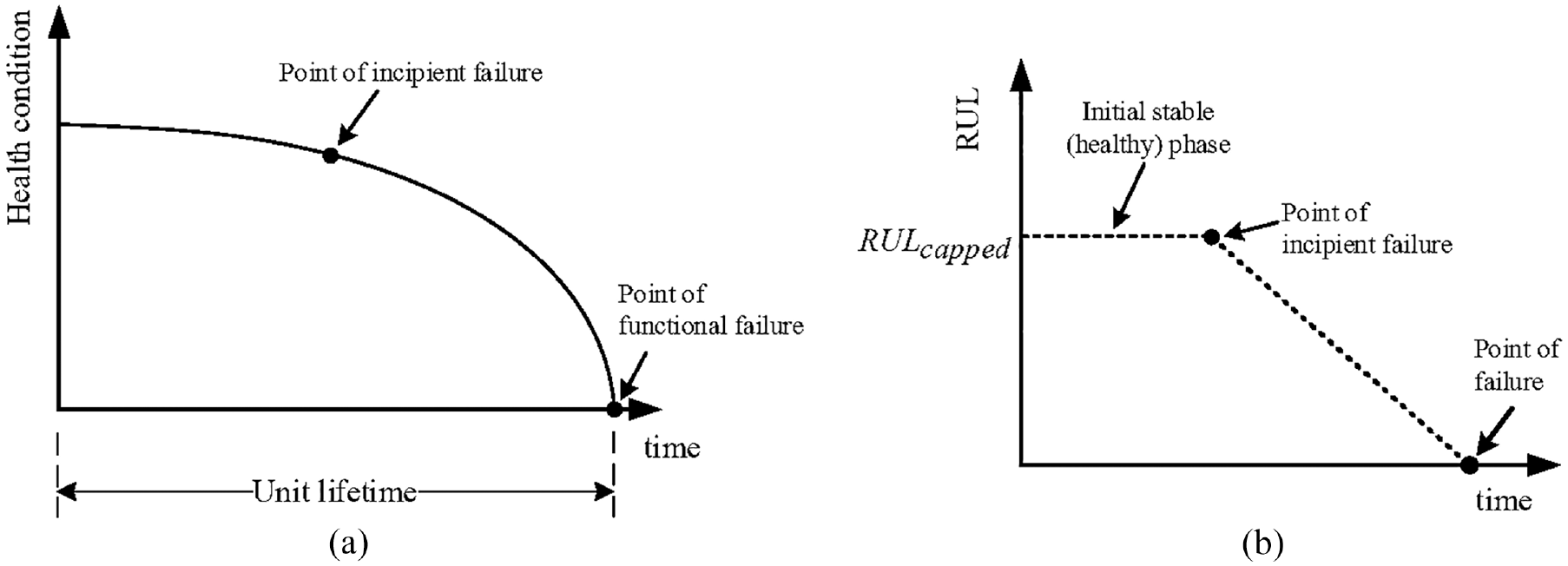
(a) Typical degradation of a component represented by P-F curve and (b) modeling of RUL for the training data.

A flowchart depicting the RUL prediction process using the model is shown in Figure 4.

Figure 4.

Flowchart showing the RUL prediction process.

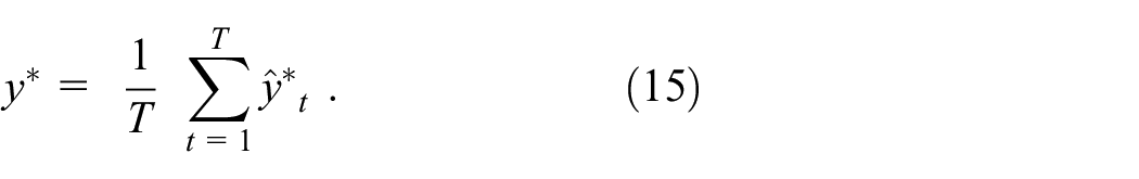
The mean RUL, ${\mu }_{\mathrm{RUL}}$ , is equivalent to the Bayesian predictive distribution, $p(y|x_{\mathrm{test}},\mathcal{D})$ . Regarding the uncertainty, since T was chosen to obtain statistical significance, the credible interval, CI, is obtained to be equivalent to 95% of the confidence interval if the distribution were normal (i.e. ±1.96σ). However, in the case of the MC dropout algorithm, the CI corresponds to the quantiles at 0.025 and 0.975, which can also be obtained by calculating the percentiles, with the upper bound being the value in the predicted distribution which is greater than 97.5% of all outcomes while the lower bound is the value less than 2.5% of all outcomes.

Case study

In this Section, the proposed BNN model with the MC dropout method is applied to quantify the uncertainty of RUL predictions for NASA’s turbofan engine degradation simulation dataset (CMAPSS). ⁶⁷ This dataset was chosen as it is publicly available and well-researched, and it builds on our previous research paper. ⁶⁴ It also lends itself to ease of comparison to other similar prediction methods. The implementation details are provided in the following sections, and the results are reported and discussed:

Data description

NASA’s Commercial Modular Aero-Propulsion System Simulation (C-MAPSS) is a tool for the simulation of large commercial turbofan engine data. The tool contains four run-to-failure datasets under different fault modes and varying operational conditions. The training sets commence at a point where all units are in a healthy state and end at the point of failure for each unit. For the test sets, the data for all units commence when each unit is in a healthy state and are terminated at an unknown point during each unit’s lifetime. For more details about the dataset, the readers can refer to Saxena et al. ⁶⁸ For this study, the dataset FD001 is used. This dataset contains run-to-failure data for 100 identical turbofan engines subjected to similar failure modes and same operating conditions. There is a separate training data which is used for model training and validation, while there is also a separate test data which is to be used to predict the RUL for the 100 engine units by means of the trained model. For both the training and the test data, each of the 100 engine units has a distinct lifetime, with three columns representing operational condition settings and another 21 columns representing sensor data. These parameters, that are taken as condition monitoring variables indicating the engines’ degradation, are presented in Table 1.

Table 1.

Parameters in the C-MAPSS dataset.

S/N	Measured parameter	Unit of measurement	Variable assigned
1	Unit number	–	unit_num
2	Time	cycles	time_cycles
3	Operational setting 1	–	ops_set1
4	Operational setting 2	–	ops_set2
5	Operational setting 3	–	ops_set3
6	Total temperature at fan inlet	°R	s_1
7	Total temperature at LPC outlet	°R	s_2
8	Total temperature at HPC outlet	°R	s_3
9	Total temperature at LPT outlet	°R	s_4
10	Pressure at fan inlet	Psia	s_5
11	Total pressure in bypass-duct	Psia	s_6
12	Total pressure at HPC outlet	Psia	s_7
13	Physical fan speed	rpm	s_8
14	Physical core speed	rpm	s_9
15	Engine pressure ratio (P50/P2)	–	s_10
16	Static pressure at HPC outlet	Psia	s_11
17	Ratio of fuel flow to Ps30	pps/psi	s_12
18	Corrected fan speed	rpm	s_13
19	Corrected core speed	rpm	s_14
20	Bypass Ratio	–	s_15
21	Burner fuel-air ratio	–	s_16
22	Bleed Enthalpy	–	s_17
23	Demanded fan speed	rpm	s_18
24	Demanded corrected fan speed	rpm	s_19
25	HPT coolant bleed	lbm/s	s_20
26	LPT coolant bleed	lbm/s	s_21

Data processing

This section briefly describes the preprocessing of the data, which formed the basis for features selection. First, the statistics (mean, median, variance, standard deviation) for each of the sensor readings are calculated to gain quick but useful insights about the data. Then, the sensor readings with zero variance are eliminated as they do not provide any useful information. As such, seven sensors, s_1, s_5, s_6, s_10, s_16, s_18, and s_19, all of which have zero variances, are eliminated. After that, the data from remaining 14 sensors are scaled using Min-Max normalization technique and the scaled data is smoothed using a robust locally weighted scatterplot smoothing algorithm as proposed in the study of Cleveland. ⁶⁹ Finally, the sensor readings are further reviewed to find out which one has been most informative for prognostics purposes. To achieve this, the prognosability, trendability, and monotonicity metrics are computed on MATLAB, and in accordance with the work of Coble and Hines,^70,71 a fitness value is defined as in equation (17) by combining the values of all three metrics:

$$\mathbf{fitness}=\mathbf{prognosability}+\mathbf{trendability}+\mathbf{monotonicity}$$

(17)

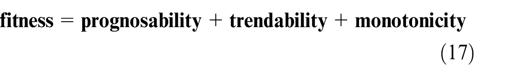
Table 2 presents the fitness values calculated for 14 sensors.

Table 2.

Fitness values for selected 14 sensor data.

Sensor	s_2	s_3	s_4	s_7	s_8	s_9	s_11
Fitness value	2.81	2.78	2.83	2.84	2.04	0.97	2.87
Sensor	s_12	s_13	s_14	s_15	s_17	s_20	s_21
Fitness value	2.89	2.09	0.96	2.82	2.80	2.87	2.79

Given that prognosability, trendability, and monotonicity metrics have values in the range of [0,1], the range of the fitness value will be between 0 and 3. A selection criterion is then set to choose sensors with the best predictive information. By applying the selection criterion: fitness ≥ 2.0, 12 sensors of s_2, s_3, s_4, s_7, s_8, s_11, s_12, s_13, s_15, s_17, s_20, and s_21 are exported for use in training the BNN model. A plot of the smoothed data for the 12 selected sensors for sample engine units (units 5 and 12) is depicted in Figure 5, revealing that most sensor trends are either predominantly monotonically increasing or monotonically decreasing.

Figure 5.

Scaled and smoothed sensor data for units 5 and 12.

Hyperparameter tuning and BNN training

With the preprocessed data imported on TensorFlow, the negative log likelihood is defined as the loss function using the log_prob function available on TensorFlow Probability while the softplus function is used to constrain the trainable scale (or variance parameter) to a positive value. To model the RUL, the values are capped at 125 cycles which proves to yield the most optimal results after several iterations. Afterward, the deep BNN is tuned using the Hyperband class in Keras tuner, with the first and penultimate layers of the network fixed at 256 units. This is done to control the width of the network while optimizing the network’s depth. This leads to the selection of the “best hyperparameter” values of 992 units in each of the 5 tunable hidden layers, a dropout rate of 0.1, and a learning rate of 0.001 for the Adam optimizer. With the network fully configured using these values, the Keras tuner is then used, along with the training data, which has been split into 85% training data and 15% validation data, to iterate and obtain the optimal number of epochs (or “best epoch”) as 83, which may vary slightly depending on training, especially with the stochasticity introduced by the MC dropout method. The fully defined deep BNN is then used to train the network.

Regarding the evaluation of the effect of different hyperparameters on the model performance, ablation studies can provide useful insights. However, this may require tweaking the base algorithm used for the model and may detract from the “best hyperparameters” that have been tuned by the algorithm using the training and validation data. A possible area of additional investigation would be to see how different tuners affect the overall model’s parameters or the performance derived from tweaking parameters on the basis of ablation studies versus the performance achieved using the hyperband tuner.

• (i) Prediction results: The model is run using Colab Pro, which provides access to GPUs and Virtual Machines on Google Compute Engine’s backend. Runtime for the algorithm including the hyperparameter optimization process was 829 s. When the model is built with the selected hyperparameters, the runtime is reduced to 490 s. With a Bayesian deep learning model, complexity increases since the learning process leads to the prediction of both the mean RUL and the credible intervals. Huge computing resources are therefore required, hence the use of GPUs. Runtime more than quadruples when run on a regular high-end CPU with 16 GB RAM. The obtained runtime results are comparable with those obtained in other studies using Bayesian methods on the same dataset; 1300 s, ³⁶ and 121 s. ⁵³

In accordance with the MC dropout algorithm, RUL predictions with uncertainty quantification are made by making T = 1000 passes of the test data through the trained BNN. The mean RUL, ${\mathrm{\mu }}_{\mathrm{RUL}}$ , is obtained using equation (16) while the upper and lower bounds of the credible intervals, CI, are obtained as the quantiles at 0.975 and 0.05 respectively (corresponding to percentiles at 97.5% and 5% respectively). The RUL prediction results obtained for the 100 units are given in Table 3. The fundamental goal in prognostics is to ensure that faults in critical equipment are identified and their future failure times are estimated so that an appropriate maintenance strategy can be planned and implemented in advance before any failure occurs. As such, the focus here will be on the units with ground truth RUL of 60 cycles or less (the range of the ground truth RUL is between 7 and 142 cycles).

Table 3.

Predictions for 100 units in FD001 dataset (RUL and CI units are in number of cycles).

Unit #	RUL t	σRULp	(σRULp + CI)	(σRULp − CI)
1	112	113	131	90
2	98	46	59	33
3	69	20	43	6
4	82	54	73	40
5	91	55	69	39
6	93	125	131	117
7	91	122	136	101
8	95	81	107	63
9	111	24	35	14
10	96	104	138	60
11	97	19	36	6
12	124	136	148	121
13	95	122	131	112
14	107	67	86	51
15	83	109	131	86
16	84	127	135	119
17	50	53	65	41
18	28	38	50	27
19	87	125	132	118
20	16	41	54	29
…	…	…	…	…
…	…	…	…	…
…	…	…	…	…
81	8	11	21	1
82	9	5	13	0
83	137	55	76	41
84	58	85	109	65
85	118	107	124	91
86	89	99	116	81
87	116	133	143	122
88	115	100	122	63
89	136	53	69	41
90	28	30	46	17
91	38	38	50	27
92	20	3	11	0
93	85	24	35	15
94	55	69	87	55
95	128	106	125	83
96	137	123	129	116
97	82	70	90	55
98	59	60	83	40
99	117	125	133	118
100	20	54	65	42

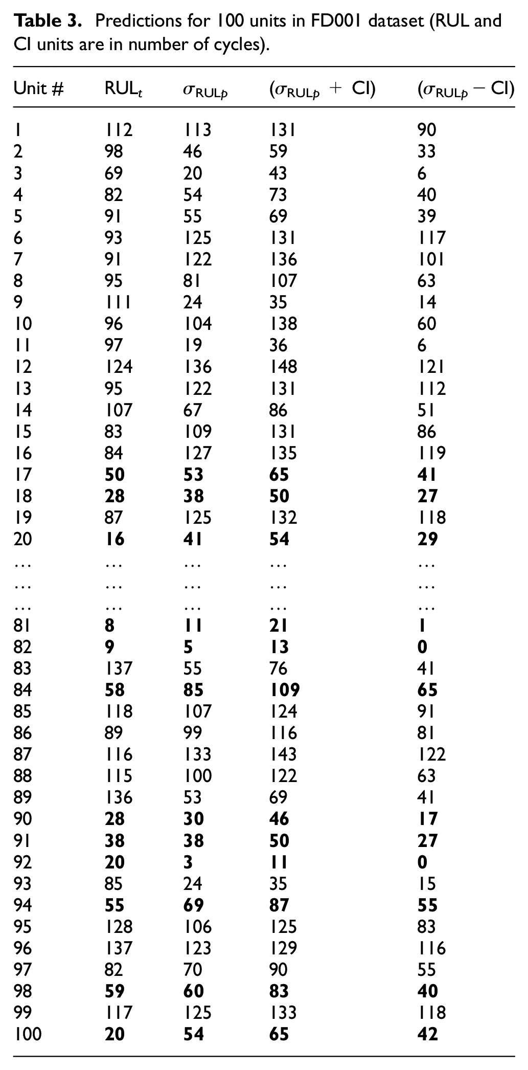
In Table 3, all the units with RUL_t ≤ 60 cycles are in bold text. Out of the 39 engine units with RUL_t ≤ 60, the ground truth RUL for 24 units falls completely within the range of the RUL prediction along with the uncertainty bounds, the true RUL for 2 units falls just a few cycles outside the prediction boundary while the remaining 13 units have predictions outside the uncertainty bounds. This is a good result at 95% confidence level. Most importantly, predictions do not make assumptions of certainty as it is with point estimates. To provide further insight into the prediction results, Table 4 shows a comparison of RMSE (root mean squared error) values for the proposed method, against other methods, most of which, however, provide only point estimates of predictions on the FD001 dataset.

Table 4.

Comparison of prediction performance for different methods on the FD001 dataset.

Method	Reference	RMSE (# of cycles)
Proposed (BNN via MC dropout)	–	38.94
Convolutional Neural Network (CNN)	Coble and Hines 70	18.45
Long Short-Term Memory (LSTM)	Coble and Hines 71	16.14
Multi-Objective Deep Belief Networks Ensemble (MODBNE)	Babu et al. 72	15.14
Bi-directional LSTM	Zheng et al. 73	14.26
Bayesian LSTM	Kim and Liu 36	12.19
Deep CNN with Bayesian Optimization and Adaptive Batch Normalization	Li and He 53	11.94
Bayesian Neural Networks using variational inference (VI) and Hamiltonian Monte Carlo (HMC)	Zhang et al. 74	HMC: 20.84; VI: 21.80

As can be seen, BNNs are designed to minimize the negative log likelihood, with the algorithm accounting for both epistemic and aleatoric uncertainties; hence, relatively high RMSE is obtained when using the mean RUL as the only basis for performance measure. Making such comparisons, however, does not account for the advantage that uncertainties have been incorporated into the BNN prediction model and that the results obtained would be more beneficial to engineers in terms of planning for maintenance actions. As an additional part of the discussion regarding the prediction results, a crucial note is again made here that conventional algorithms that make point estimates use metrics like RMSE, MAE (mean absolute error), or a scoring function developed for use with the CMAPSS dataset. Most studies published in the literature also use the RMSE metric for measuring the performance of BNN algorithms in predicting RUL. However, since the optimization objective for BNNs is the minimization of negative log likelihood, the use of RMSE as a performance measure is somewhat inappropriate. Therefore, there is a need to develop bespoke metrics for use in measuring BNN performance. Given that BNNs can quantify uncertainty, some attempts have been made to use the average variance or average standard deviation (i.e. the average confidence interval or average uncertainty) as a performance measure. This is comparable to the Overall Average Variability (OAV) metric presented in the work by Zemouri and Gouriveau. ⁷⁵ The average CI obtained for the prediction results from this study is 38.78 cycles. Such a measure will be useful for benchmarking or comparison with other methods when the dataset is same or the number of passes through the algorithm during prediction is same or at least normalized, so that aleatoric uncertainty is constant, and the performance of epistemic uncertainty quantification can then be assessed and compared. Another metric that may be suitable for measuring the predictive performance of BNNs used for RUL prediction is the Confidence Interval Coverage (CIC), as presented in the work by Sharp. ⁷⁶ The CIC measures the number of predictions for which the RUL falls completely within the confidence bounds, as a percentage of the total number of predictions. Achieving a CIC of 100% would mean that all the predictions fall completely within the confidence bounds. The CIC value will increase when the confidence level drops from 95% to 90% and would increase further as the confidence level decreases further. Using this metric, which is rather simplistic, an average CIC value of around 60% will be achieved, over several runs of the algorithm at 95% confidence level. Again, this is an evolving area, and a clear gap exists for additional research toward measuring performance of BNNs, to achieve a robust benchmarking of prediction results against results from other studies. Consequently, the focus of this study is on the practicality of using prediction results by engineers and the interpretability that the results offer, when compared to point estimates.

• (ii) Engine degradation trajectories: The RUL prediction trajectories are obtained, and the results show that our modeling is correct. Figure 6 represents the RUL prediction trajectory plots for nine random engine units, with the main selection criterion being that each unit has reasonably degraded, and it is approaching the end of life. As can be seen from all nine plots, the RUL remains fairly steady at the commencement of each unit’s operation. However, a clearly noticeable point is reached along the trajectory where the rate of decline increases; this point corresponds to the point during operation of the engine when a fault is detected by sensors. In fact, even when the RUL is modeled linearly and the network is trained using the linear RUL, the RUL trajectory for some engines shows this characteristic. This shows that the deep BNN is able to decipher, from the sensor data, when a fault has occurred in any of the engines.

Figure 6.

Predicted degradation trajectory for nine random engine units.

Regarding uncertainty quantification, by sampling the mean RUL for T times, where T = 1000 in our study, 1000 possible combinations of the network model weights are accounted for. T, which represents the number of prediction iterations of the algorithm for each set of input, is chosen to achieve statistical significance and obtain a distribution spread that captures most prediction outcomes. In other ML algorithms that adopt the MC dropout method, typical values for T lie in the range of 200–500, which equally produce several runs of the algorithm that achieve statistical significance. For this study, T was chosen as 1000 to ensure diversity in the results obtained, thus ensuring that the true RUL distribution is better captured. As such, the Monte Carlo sampling implemented by the BNN inherently accounts for the epistemic uncertainty as the variability of the predictions already accounts for the different model weights. Regarding the aleatoric uncertainty, the negative log likelihood, which is minimized as the optimization objective, involves the variance information in the data. Otherwise, the MSE, which is used for conventional regression analysis would have been used. Thus, the negative log likelihood accounts for heteroscedasticity in the RUL prediction, and the combined effect of both uncertainties can be observed in the RUL trajectories in Figure 6, with varying prediction uncertainty as the degradation trajectory progresses. Another important observation from Figure 6 is that the uncertainty bounds taper inwards and narrow as each unit’s end of life approaches. The reason for this is that, since the model makes RUL predictions via Bayesian inference, the confidence of predictions increases as more data becomes available, hence the typically narrower confidence bounds much later in the unit’s operational life at which time enough operational data is available to make more confident predictions.

Conclusion

The approach proposed in this study helps to bridge the gap in the literature that focuses on point estimates of the RUL instead of attempting to predict the true RUL, which are probabilistic distributions rather than deterministic point estimates. The main issue with point estimates is that they are overly confident estimates that do not account for uncertainties and can therefore be misleading, thus making the planning of maintenance tasks difficult for engineers. However, in this study, we have provided a BNN approach to RUL prediction that fully accounts for both aleatoric and epistemic uncertainties and the results obtained are more interpretable for engineers and thus a lot more useful in practical terms for decision making. The Bayesian approach used fundamentally indicates where and when the prediction model is not very confident, based on the data available and the model used for prediction. Uncertainty is quantified in numerical terms rather than qualitatively, thus providing interpretable information in terms of the mean and credible intervals of the RUL, which in turn help to determine the lead time to making maintenance decisions. Thus, the results obtained from this study are very useful inputs for spares management, maintenance logistics planning and end-of-life management of high-value assets.

It must however be emphasized that uncertainty quantification in prognostics and health management (PHM) of industrial assets remains an on-going challenge. The practice of PHM has continuously evolved with time and in the era of big data, the use of condition monitoring technologies to optimize future asset maintenance decisions has been extensively explored, leading to several methodologies that have proved their usability for predicting RUL of engineering equipment. For BNNs, one of the assumptions made about the true posterior distribution in uncertainty quantification is that the true RUL follows a Gaussian distribution. Even though the MC dropout approach used in this study seems not to explicitly make the same analytical assumption of the posterior distribution, the negative log likelihood, which is the optimization objective, implicitly assumes that the posterior is a Gaussian. As such, a possible improvement area as regards uncertainty quantification in RUL prediction is an algorithm that is completely agnostic to the true posterior distribution, since the true RUL posterior distribution indeed may not always be Gaussian. Also, performance measurement for BNNs is an ongoing research area, given that the algorithm yields uncertainty bounds which characteristically have different spreads and their accuracies are not easy to measure using conventional metrics as applied in regression problems, like the RMSE. Metrics such as the Confidence Interval Coverage (CIC) and the Overall Average Variability (OAV) have been suggested in the literature to address performance measurement for algorithms that incorporate uncertainty quantification. Developing applicable metrics will aid an easy comparison between different prognostics results for similar datasets or even across disparate datasets. The ideal goal will be to develop models that provide very narrow uncertainty bounds at high confidence levels and then measure their performance using bespoke metrics.