Sage Journals: Discover world-class research

Abstract

The Rankine cycle is a conceptual arrangement of four processes as a closed vapor power thermodynamic cycle, where a working fluid (especially water as a liquid, as a vapor, and as a liquid-vapor mixture) can be used to convert heat into mechanical energy (shaft rotation). This cycle and its variants are widely used in electric power generation through utility-scale thermal power plants, such as coal-fired power plants and nuclear power plants. In the steam-based Rankine cycle, water should be pressurized and heated to be in the form of very hot high-pressure water vapor called “superheated steam,” before the useful process of expansion inside a steam turbine section occurs. If the absolute pressure and temperature of the superheated steam are both above the critical values for water (220.6 bara and 374.0°C), the cycle is classified as “supercritical.” Otherwise, the cycle is classified as “subcritical.” This study considers the impact of the temperature and pressure, independently, on the performance of a steam Rankine cycle. Starting from a representative condition for a subcritical cycle (600°C peak temperature and 50 bara peak absolute pressure), either the peak temperature or the peak absolute pressure of the cycle is increased with regular steps (up to 900°C, with a temperature step of 50°C, and up to 400 bara, with a pressure step of 50 bar). The variation of five scale-independent performance metrics is investigated in response to the elevated temperature and the elevated pressure. Thus, a total of 10 response curves are presented. When the temperature increased, all the five response variables were improved in a nearly linear profile. On the other hand, increasing the pressure did not give a monotonic linear improvement for each response variable. In particular, the cycle efficiency seemed to approach a limiting maximum value of 45% approximately, where further increases in the pressure cause diminishing improvements in the efficiency. When varying the peak pressure, an optimum minimum ratio of (water-mass-to-output-power) is found at 203 bara, although the cycle efficiency still increases beyond this value. In the present research work, the web-based tool for calculating steam properties by the British company Spirax Sarco Limited, and the software program mini-REFPROP by NIST (United States National Institute of Standards and Technology) were used for finding the necessary specific enthalpies (energy content) of water at different stages within the steam cycle. Both tools were found consistent with each other, as well as with the Python-based software package Cantera for simulating thermo-chemical-transport processes. The results showed that if the peak temperature reaches 900°C, a gain of about 5 percentage points (pp) in the thermal cycle efficiency becomes possible (compared to the case of having a base peak temperature of 600°C), as the predicted efficiency was found to increase from 38.60% (base case) to 43.67%. For the influence of the steam peak pressure, operating in the subcritical regime but close to the critical point appears to be a good choice given the gradual decline in efficiency gains at higher pressures. About 4.7 percentage point increase was found at the high subcritical peak pressure of 200 bara (compared to a base subcritical peak pressure of 50 bara). The results of this study also showed that the liquid water droplet mass fraction at the steam turbine exit diminishes from 11.00% at 600°C to only 1.48% at 900°C, which is favorable. This mass fraction grows from 11.00% at 50 bara to 27.89% at 400 bara, which is not acceptable. Every 100°C increase in the superheating temperature between 600°C and 900°C was found to cause aa increase in the cycle thermal efficiency by about 1.69 percentage points, and simultaneous a beneficial increase in the steam quality at the turbine exit by about 3.17 percentage points.

Keywords

Steam Rankine superheated power plant mini-REFPROP Spirax Sarco

Introduction

Background

Electricity is a crucial element of the modern civilization. While renewable energy sources gradually replace conventional ones (non-renewable sources: fossil fuels and nuclear fuels) for producing electricity at large scales, conventional sources may be in use for many years for electricity generation. In 2019, the share of conventional energy sources in electricity generation was 73.6% (63.2% fossil fuels and 10.4% nuclear fuels), and the remaining 26.4% came from renewables.¹ The 2030 target share of renewables in the final energy consumption in the European Union was set to 32% in 2018, which is subject to a revised increase to 45% as per the 2020 REPowerEU Plan.² Most of the electricity generated in the USA is from steam turbines using fossil fuels, nuclear fuels, biomass, geothermal energy, and solar thermal energy.³ These numbers show that despite the ambitions to intensify renewables, conventional energy sources and conventional electricity generation (which is related to the topic of this research) are not expected to cease in the near future.

One of the technologies for generating electricity in power plants is the use of a steam power cycle (a Rankine cycle). The term “cycle” or “thermodynamic cycle” here refers to a sequence of processes (changes) applied to a working medium where the final state is identical to the initial state. Other thermodynamic cycles are used in refrigeration, such as the vapor compression cycle, in which the working medium can be a hydrofluorocarbon (HFC) refrigerant fluid, such as R134A.⁴ A steam power cycle (where steam is used to rotate steam turbines) can be combined with a Brayton power cycle (where combustion product gases are used to rotate similar gas turbines). A power plant utilizing such a dual-cycle system is referred to a combined cycle power plant.⁵

Steam (or hot water vapor) can exist in multiple forms, all of which are generically referred to as “steam.” To further distinguish these forms, specialized terms are used. When steam has just been generated by boiling liquid water which is converted into a gaseous phase; once the last droplet of liquid is vaporized by the effect of heat, the resulting steam is specifically called “saturated vapor” or “dry steam.”⁶ If this freshly-formed hot water vapor is heated further while it is in the gaseous phase, it is called “superheated steam” provided that its pressure does not exceed a special value called the critical pressure of water, which is a physical constant equal to 220.6 bara,⁷ and this is about 217.7 times the atmospheric pressure.⁸ If the water is heated while it is also compressed (pressurized) to a high pressure above the critical pressure for water such that its temperature exceeds another water-specific constant called the critical temperature of water, which is 374.0°C ⁹; this water is described as “supercritical water” or “supercritical fluid.”¹⁰ What is unique about this form of water is that it does not exhibit a liquid-to-vapor or a vapor-to-liquid phase change at a constant temperature. Instead, it represents an intermediate condition between a liquid and a vapor.¹¹ It may be viewed as a liquid that is very light, or as a vapor that is very dense. Supercritical water is not classified purely as a liquid or as a vapor, and it is not a liquid-vapor mixture (but a homogenous fluid medium). Superheated steam has more energy content than saturated vapor steam, due to the additional acquired heat. Supercritical water has even more energy content than superheated steam due to the elevated pressure, which also means more energy content per unit mass of water. Thus, using superheated steam in power plants is preferred than using saturated vapor, because it allows extracting more energy from the same mass of the heated gaseous water. Similarly, using supercritical water is preferred over using saturated vapor, and can also be preferred over using superheated steam,¹² when the usefulness of water as an energy carrier is concerned. In the present study, the term “superheated steam” is used also when referring actually to supercritical water, not just to superheated steam. This simplifies the presentation of results. However, the reader should be aware that when the critical pressure and temperature are both exceeded in some of the simulation cases reported here, the term “supercritical water” becomes more appropriate to use to refer to the water. In all the simulation cases here, the critical temperature of water is exceeded after the boiler section of the modeled steam cycle. Thus, in these simulations, exceeding the boiler pressure is sufficient to have supercritical water after the boiler section (which means before the turbine section). A subcritical Rankine steam cycle is the traditional (default) version of the Rankine steam cycle,¹³ where water is not compressed high enough to a level exceeding the critical pressure of water when it is sent to the turbine section for power extraction. Water is either saturated vapor or superheated steam (but not supercritical fluid) when it is at its peak temperature and pressure within subcritical Rankine cycles. In the present study, water is always superheated steam (rather than saturated vapor) in the subcritical Rankine cycles before the turbine section (thus, when water is at its peak pressure and temperature). On the other hand, when water is both compressed and heated enough to exceed both the critical pressure and the critical temperature when it is sent to the turbine section (thus, water enters the turbine as a critical fluid), this steam cycle is then designated as a supercritical cycle.

In the steam power cycle, the working medium is water, changing its state repeatedly in a closed loop. During this steam power cycle, water is compressed using one or more water pumps, and then is heated in a boiler (or another device, such as a solar concentrator or a heat recovery steam generator, HRSG) to a state of hot water vapor (steam), which is then allowed to expand in one or more steam turbines to produce mechanical shaft energy (shaft rotation). This rotation is used later to drive one or more electric generators.¹⁴ The expanded steam returns back to its original state (as saturated liquid water) using one or more condensers. It is then sent again to the pump section, and the cycle is repeated. The source of heat in the steam cycle can be from a fossil fuel,^15,16 a nuclear fuel,^17,18 biomass,¹⁹ or a concentrated solar power system, which collects solar radiation and utilizes it as a clean source of heat.^20,21 For example, a recent study²² analyzed the use of the renewable solar energy through parabolic trough concentrators (which are curved mirror elements used to collect and reflect solar radiation while concentrating it onto a small zone) for use in the Tashkent power plant in Uzbekistan. The Tashkent power plant has an electric power capacity of 2240 MW. It uses both steam turbines and gas turbines. The superheated steam pressure is 140 bara, with a temperature of 545°C. In their computer modeling and simulation for the proposed concept of a solar-fossil hybrid power plant, the steam cycle takes its needed heat partly from burning a fossil fuel, and partly from solar heating. The fossil fuel used for steam generation in that power plant is natural gas. Despite this flexibility in the heat source, the term “boiler” is used in the current study as a genetic name for the subsystem in the steam cycle that is responsible for transferring heat to the water, thereby converting it into superheated steam.

The design and operation of a steam cycle involves the selection of various parameters, which affect the performance of the cycle. Optimizing some of these parameters or the components of a steam-based power plant through research studies helps in reducing the input heat energy needed, and thus in reducing the consumed fuel (in the case that fuel combustion is the method of generating the required heat energy for operating the steam cycle) for generating the same amount of electricity output.²³

The design parameters of a steam cycle include the temperature and pressure of the superheated steam (thus, the temperature and pressure of the steam as it exits a boiler and enters a steam turbine). The superheated steam temperature is here referred to as the “superheating temperature.” The boiler is assumed to have a constant pressure. Thus, the superheated steam pressure may also be referred to as the “boiler pressure.” The superheating temperature is the peak temperature value in the entire Rankine cycle. Similarly, the boiler pressure is the peak pressure value in the entire Rankine cycle.

Khaleel et al.²⁴ performed a parametric study, through which they examined the impact of the superheated steam pressure on the effectiveness of feedwater heaters (FWH) for a numerical model corresponding to unit 1 of the Manjung coal-fired power plant located in Malaysia, which utilizes a steam power cycle, and has a nominal electric power capacity of 700 MW. Feedwater heaters are auxiliary components in a steam power cycle for partially heating liquid water before it is sent to the boiler for the main heating stage. In their methodology, they used the Engineering Equation Solver (EES) commercial software²⁵ in their computational modeling. Although their considered steam cycle is more complicated than the one considered here (e.g. the single steam turbine here is replaced in their model by four steam turbines), it is pleasant that their predicted thermal cycle efficiency with 100 bara is nearly 42.4%, which agrees with value obtained in the current study (41.15%) at 100 bara. They also examined the resultant variation in the mass flow rate of consumed coal, and the power delivered by the steam cycle. The range of examined pressures was 100–200 bara. In their study, they examined also the influence of the superheating temperature (the high temperature of steam as it leaves the superheater, which is the peak temperature of steam within the cycle), over the range 539.8°C–580°C. Despite the valued information provided by their work, the current study may be viewed as an extension to their work through: (1) expanding the range of peak superheated steam pressure, (2) expanding the range of peak superheated steam temperature, (3) showing the variation of additional performance variables, and (4) simplifying the cycle design, which makes the results less specific to one design.

In another study,²⁶ the EES software was used to examine multiple effects of the turbine inlet temperature (TIT), the ambient temperature, and the condenser pressure for the unit 1 of Manjung coal-fired power in Malaysia. The turbine inlet temperature is the peak temperature of the superheated steam as it leaves the superheater. The steam-based model for the power plant has three sequential turbine stages (high pressure stage, intermediate pressure stage, and low pressure stage). The range of turbine inlet temperatures was 540°C–360°C. The range of ambient temperatures was about 23°C–63°C, and the range of condenser pressures was 0.03–0.2 bara. It was concluded that increasing the condenser pressure from 0.03 bara to 0.20 bara causes a decrease in the power output from the steam cycle by 1.53% (from 594.799 MW to 585.676 MW). In the current study, the condenser pressure is 0.125 bara, which is within the examined range in their study. It is a fixed parameter in the present study, which focuses on the impact of TIT and the peak steam pressure. The condenser pressure seems to have a limited influence; it has a narrow range of possible values because it is subject to a theoretical lower limit of 0 bara.

Goal of the Study

The goal of this research is to investigate the improvement in the performance of a Rankine cycle due to increasing the peak temperature or the peak pressure of the steam utilized in the cycle, beyond a reference base value. The base superheating temperature in the current study is 600°C,^27–29 and the base boiler pressure in the current study is 50 bara.^30,31

Other fixed operational conditions are the condenser pressure, which is set to 0.125 bara.³² The condenser operates under saturation conditions, which means that specifying a constant pressure value implies also a specified constant temperature of water inside the condenser, which is gradually transformed from a liquid-vapor mixture state into a fully-liquid (saturated liquid) state. Therefore, setting the pressure value for the condenser automatically determines the temperature value of the water inside condenser, which is 50.24°C. This saturated liquid water is compressed inside the pump section, which is assumed to be isentropic (thus, no change in the specific entropy through it). Therefore, the temperature of the compressed liquid water (subcooled liquid water) leaving the pump section at a specified boiler pressure can be determined uniquely.

The investigated range of superheating temperature is from 600°C (the base case) to 900°C, with an interval of 50°C. Thus, a total of seven temperature values are studied, including the reference base case. The investigated range of absolute boiler pressure is from 50 bara (the base case) to 400 bara, with an interval of 50 bar. Thus, a total of eight pressure values are studied, including the reference base case.

To properly quantify the impacts of the superheating temperature or the boiler pressure on the performance of the steam power cycle, a number of quantitative standardized (thus, not dependent on the scale of operation and the amount of power to be generated) response variables were selected as indicators of the cycle performance. These performance response variables are:

Cycle thermal efficiency (the higher the value, the better the performance)

Steam quality at the turbine exit (the higher the value, the better the performance)

Specific input heat (heat added to each kg of water)

Specific net output shaft work (net output mechanical shaft work from each kg of water)

Mass flow rate of water needed to generate 1 GW electric power, assuming 10% losses in the shaft power when converted into electric power (the lower the value, the better the performance)

The third and fourth performance variables in the above list (specific heat and specific net output work) are not individually enough to evaluate the performance of the cycle, because having a higher input heat alone does not necessarily mean that the performance is better. It is the ratio of these two response variables (giving the cycle efficiency) which forms a meaningful measure of excellence. Despite this, these two specific values are still presented and included in the study, because examining them helps in interpreting the variation in the cycle efficiency. The fifth performance variable is an auxiliary result, and is not part of the core analysis. However, it can still be a useful way to express the real water needs for a power plant (rather than an isolated steam cycle). Due to the linear relation between this estimated need of water flow and the electric power, the value of this fifth performance variable can be conveniently scaled to fit a power level other than the selected reference value of 1 GW. For example, half of the presented mass flow rate of water should be considered if the power of interest is 0.5 GW (500 MW) of electricity rather than 1 GW.

In addition to the cycle thermal efficiency, another derived efficiency is presented, which is the power plant efficiency. It represents the result of dividing a hypothetical electric power output from a power plant that utilizes the steam cycle by the input heat to that steam cycle. While such auxiliary power plant efficiency is not employed in the modeling analysis itself (but a post-processing derived quantity), it can be more convenient for readers concerned with power plant technologies other than steam cycles, such as wind energy. The provided power plant efficiency in this case allows benchmarking. The power plant efficiency (η_p) in the current study is assumed to be related to the cycle thermal efficiency (η_c) according to a simple multiplicative loss factor, or energy conversion efficiency (η_v), which is selected to be 90%.³³ This means that 10% of the net output shaft power is assumed to be lost when converted into electric power. The sources of losses can be electric generator loss, unintended heat transfer losses,³⁴ and friction.

Article structure

In the next section, the research method is described. Next, another section is provided for describing the water states and the governing equations employed. Then, some details about the base case are summarized. After this, the impact of the superheating temperature on the steam cycle performance is provided and examined. Following this, the impact of the boiler pressure on the steam cycle performance is provided and examined. Finally, concluding remarks are provided.

Problem statement and main objective

The issue addressed in this research study is a desire to examine quantitatively the independent influence of peak pressure and peak temperature on the performance of a typical steam power cycle, with developed mathematical fitting models, such that a designer can take this into consideration when selecting a design point. This is the main objective of the current investigative work.

Research method

Models

The results of this study have been reached through mathematical thermodynamic modeling, by applying open-system energy balance equations to the four devices of the Rankine cycle (pump, boiler, steam turbine, and condenser), followed by a whole-cycle analysis. Numerical analysis is performed, with the aid of water properties obtained from computer applications.

Source of water properties

The analysis of the steam cycle needs properties of water at its different states inside the cycle. These four states are 1: after the condenser and before the pump, 2: after the pump and before the boiler, 3: after the boiler and before the steam turbine, and 4: after the steam turbine and before the condenser. The main thermodynamic property needed is the specific enthalpy. The other supplementally property that was needed during the analysis is the specific entropy, as a means to relate two states at the ends of an isentropic process (namely states 1 and 2, and states 3 and 4). The properties were obtained for some cases using the online steam calculator provided by Spirax Sarco Limited, which is a British company working in the field of steam.³⁵ This web application was made gratefully available for use free of charge by its owner. It was used in the base case and in the cases when the superheating temperature was incrementally increased. Despite the extensive details provided by this online steam calculator, its pressure range made it unsuitable for examining the effect of the boiler pressure in the current study. In particular, when an absolute pressure of 150 bara was attempted for state 2 (after the pump), no results were returned due to a limitation on the rage of permitted pressure values. Therefore, another steam calculator was used when investigating the effect of boiler pressure. This second source of water properties used here is the mini-REFPROP software program that was gratefully made freely available by NIST – the United States National Institute of Standards and Technology.³⁶ The version used here is 10.0. There is big consistence between the two steam calculators. For example, using the online calculator of Spirax Sarco at the base temperature (600°C) and the base pressure (50 bara) of the superheated steam gave a specific enthalpy of 3666.330 kJ/kg, and a specific entropy of 7.26064 kJ/kg.K. On the other hand, the NIST offline steam calculator for the same conditions gave a specific enthalpy of 3666.839 kJ/kg, and a specific entropy of 7.26051 kJ/kg.K. The two pairs of values are nearly identical. The relative difference is below 0.014% for the specific enthalpy and below 0.0018% for the specific entropy, making the deviations approximately zero. The NIST calculator has the advantage of handling a wider pressure range, including supercritical values (beyond 220.6 bara). Therefore, it was used when examining all the cases of elevated boiler pressures (from 100 bara to 400 bara).

Selection of references

The selection of references for this work was stimulated by the need to support various data elements presented in the current research study, either for results directly generated through the conducted simulations, or for third-party information mentioned here. Priority was given to literature sources utilized in the analysis, because these have a larger role in justifying the performed computational modeling. Then, archival articles in relevant reputable journals are given preference for inclusion. Although some references are in the form of online resources, these web pages belong to renowned internationally-recognized organizations (such as the International Renewable Energy Agency). Thus, these sources of information were considered reliable, especially that they were accessed recently.

Governing equations

Water states

Figure 1 illustrates the four processes and four devices in the Rankine steam cycle. The pump needs input shaft work (such as from a coupled electric motor) while the steam turbine produces much larger shaft work (in the form of rotary motion of the shat). The difference is the net output shaft work. The boiler transfers heat to the water during a heat addition process to change water from compressed liquid water into superheated steam (or supercritical fluid). The condenser releases waste heat when the liquid-vapor water mixture is condensed within the condenser.

Figure 1.

Illustration of the processes and devices constituting a steam Rankine cycle.

State 1 is saturated liquid water, which takes place before the compression process inside the pump section. In this state, water is a liquid condensate formed by transforming any water vapor content (in a liquid-vapor mixture) into liquid water after leaving a steam turbine through a condensation process in a condenser. State 2 is after the compression process, where the compressed water (also called subcooled water) is ready to be sent to the boiler, after its absolute pressure has been increased from (p₁) to a higher level (p₂). The compression process is assumed to be isentropic (no change in specific entropy of water), therefore

s_{2} = s_{1}

(1)

where (s₁) is the specific entropy of water at state 1, and (s₂) is the specific entropy of water at state 2. For an absolute pressure of p₁ = 0.125 bara at state 1, the online steam calculator gives a specific entropy of s₁ = 0.7070 kJ/kg.K (and the offline calculator gives nearly the same value, 0.70692 kJ/kg.K), and the online steam calculator gives a temperature of T₁ = 50.24°C (and the offline calculator gives the same value, if four significant digits are equally retained for both calculators). The heat addition in the boiler is assumed to be isobaric (at constant pressure), thus

p_{3} = p_{2}

(2)

The water leaves the boiler in state 3 as superheated steam in subcritical steam cycles (but supercritical fluid in supercritical steam cycles). This state has the highest pressure and highest temperature in the entire steam cycle. The expansion in the turbine is assumed to be isentropic, thus

s_{4} = s_{3}

(3)

The expansion process is the useful process in the steam cycle, in which part of the enthalpic energy of the water (combination of the internal energy of water due to its temperature and the flow energy of water due to its pressure) is converted into shaft rotation. Water leaves the steam turbine section in the form of a liquid-vapor mixture (also called wet steam), which is state 4. As the temperature drops during the expansion process, some water vapor starts to condense. Having liquid droplets within the steam turbine is not desired; instead, a higher mass fraction of vapor at state 4 is desired.^37,38 It is not recommended to have a steam quality within the turbine less than about 88%.³⁹ The mass fraction of the water vapor within the liquid-vapor water mixture at state 4 is referred to as the steam quality (or the dryness fraction). It is designated by the symbol (x₄).

The vapor fraction of the water leaving the turbine is recirculated through a condenser section, such that the water is brough back to the same conditions of state 1. The condensation process is assumed to be isothermal (constant temperature) and isobaric. This means

T_{1} = T_{4}

(4)

p_{1} = p_{4}

(5)

In the current study, the temperature (T₃) and the pressure (p₃) of the superheated steam are the two controllable design variables, being subject to change incrementally from one simulation to another. As a result, the conditions at the previous state (state 2) and the following state (state 4) can also vary. On the other hand, the conditions at state 1 are fixed.

When the superheating temperature is varied as the design variable (while the pressure is kept at its base value of 50 bara), the steam cycle remains in the subcritical regime regardless of the temperature because state 3 is cannot be in a supercritical condition due to the subcritical pressure value (being less than the critical pressure of water). In these cases, the superheated steam temperature (T₃) is above the critical temperature for water, T_cr = 374.0°C,⁴⁰ but the pressure is below the critical value for water, p_cr = 220.6 bara.⁴¹ This is illustrated in Figure 2, which shows the processes paths and states of a subcritical Rankine steam cycle in the temperature-specific-entropy (T-s) diagram. When the boiler pressure is varied as the design variable (while the temperature is kept at its base value of 600°C), the steam cycle changes from subcritical (for absolute pressures p₃ = 50, 100, 150, and 200 bara) to supercritical (for absolute pressures p₃ = 250, 300, 350, and 400 bara). In the supercritical steam cycle, state 3 represents supercritical water, where both the temperature and the pressure are above the critical values, and a phase change from vapor to liquid or from liquid to vapor is not realizable. Figure 3 shows a T-s diagram for a supercritical Rankine steam cycle. Despite this change in the regime (from subcritical to supercritical), the mathematical modeling procedure is the same for either a subcritical steam cycle or a supercritical steam cycle in the presented analysis.

Figure 2.

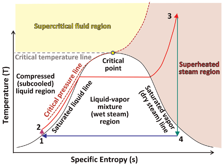
T-s phase diagram for water, showing the water states of a subcritical steam cycle.

Figure 3.

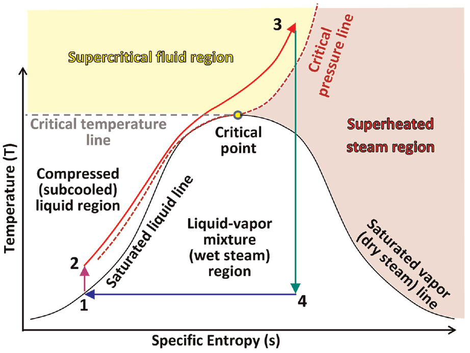
T-s phase diagram for water, showing the water states of a supercritical steam cycle.

Energy balance

When the changes in kinetic energy and potential energy in water are neglected, the energy balance becomes limited to changes in the specific enthalpy of water within each device in the steam cycle.^42,43 Each device is treated as a steady-state open system (control volume), with a single inlet and a single outlet. In this configuration, the mass balance equation is trivially satisfied by assuming a uniform mass flow rate at all stages of the cycle.⁴⁴

The energy balance equation for the pump section of the cycle is⁴⁵

w_{in} = h_{2} - h_{1}

(6)

The energy balance equation for the boiler section of the cycle is⁴⁶

q_{in} = h_{3} - h_{2}

(7)

The energy balance equation for the steam turbine section of the cycle is

w_{out} = h_{3} - h_{4}

(8)

The energy balance equation for the condenser section of the cycle is⁴⁷

q_{out} = h_{4} - h_{1}

(9)

The net output specific shaft work from cycle is⁴⁸

w_{net} = w_{out} - w_{in}

(10)

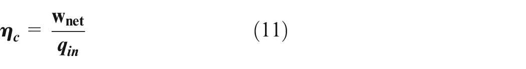
The cycle thermal efficiency is

η_{c} = \frac{w_{net}}{q_{in}}

(11)

The estimated power plant efficiency is

η_{p} = η_{v} η_{c}

(12)

The estimated specific (per unit mass of working water) output electric energy (or work) is

w_{elec} = η_{v} w_{net}

(13)

The estimated mass flow rate of water needed to operate a hypothetical power plant with an aimed electric power capacity (P) is⁴⁹

m = \frac{P}{w_{elec}}

(14)

In the above equations, all quantities have positive values; the specific heat, specific work, and specific electric work are expressed in kJ/kg, the electric power is expressed in kW (with 1 GW = 10⁶ kW), and the mass flow rate is expressed in kg/s.

Figure 4 gives a visual summary of the procedure of the cycle analysis as a flow chart. The oval (Start) and oval (End) shapes mark the beginning and the end of one complete simulation, respectively. One simulation corresponds to selected values for the design variables pair: the peak steam temperature (T₃), and the peak steam pressure (p₂, which is equal to p₃). The parallelograms in the flow chart represent known quantities that do not need computation, either because they are fixed constants in all the simulations (p₁, η_v, P), because they are selected as the independent variable to be incremented from one simulation to another (p₂, T₃), or because they are equal to another known value (s₂, p₃, s₄). The rectangular shapes represent a computation or searching step, by looking for an unknown water property directly (using either the Spirax Sarco calculator, or the mini-REFPROP program), or an arithmetic computation using one of the equations presented in the current subsection.

Figure 4.

Flow chart illustrating the steps of the computational modeling.

The specific enthalpy of water at states 1, 2, and 3 are obtained directly by the water property tool used. These do not require manual computation because water has a single phase (not a mixture of two phases, as in state 4 where water is partly liquid and partly vapor at the same time, forming a wet steam).

For calculating the wet-steam quality at state 4(outlet of the turbine), the following equation is used ⁵⁰:

x_{4} = \frac{s_{4} - s_{f 4}}{s_{g 4} - s_{f 4}}

(15)

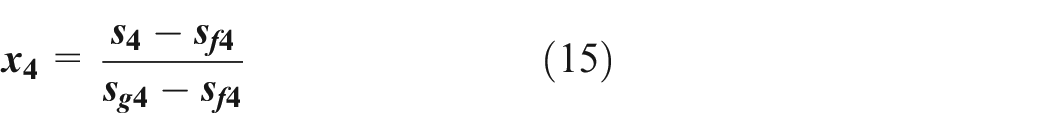
where s_f4 is the specific entropy for saturated liquid water at p₄, and s_g4 is the specific entropy for saturated vapor water at p₄. These two values are water properties that can be found from any classical steam table (alternatively, using either digital tool used in this study). At p₄ = 0.125 bara, s_f4 is 0.7070 kJ/kg.K (Spirax Sarco) or 0.70692 kJ/kg.K (mini-REFPROP), and s_g4 is 8.07080 kJ/kg.K (Spirax Sarco) or 8.0707 kJ/kg.K (mini-REFPROP).

After the wet-steam quality becomes known for the liquid-vapor water mixture at state 4, the specific enthalpy of that liquid-vapor mixture is computed as⁵¹

h_{4} = h_{f 4} + x_{4} (h_{g 4} - h_{f 4})

(16)

where h_f4 is the specific enthalpy for saturated liquid water at p₄, and h_g4 is the specific enthalpy for saturated vapor water at p₄. These two values are water properties. At p₄ = 0.125 bara, h_f4 is 209.835 kJ/kg (Spirax Sarco) or 210.35 kJ/kg (mini-REFPROP), and h_g4 is 2591.205 kJ/kg (Spirax Sarco) or 2591.7 kJ/kg (mini-REFPROP).

Results

Base case

Table 1 summarizes the water states and derived cycle performance variables for the base case. These results are consistent with results of a similar study at the same condition, but with the analysis performed using the modeling software package “Cantera” developed for incorporation as an extension library within the Python programming language to enable computer modeling of thermodynamic, chemical, or multicomponent-mixture transport problems. This package has its own database of water properties.^52–54 This is a validation for the obtained results here. For example, the predicted thermal cycle efficiency of the steam here is 38.60%, which is exact (to 4 significant digits) with the independent analysis conducted using the modeling tool Cantera. Similarly, the specific net output shaft work predicted here is 1332.111 kJ/kg, and the value obtained using Cantera is 1331.95 kJ/kg. The difference is only 0.161 kJ/kg, which is practically zero; making the two predicted values almost identical with the relative difference being 0.012%. The predicted specific input heat (to the boiler section) here is 3451.466 kJ/kg. The reported value using Cantera is 3450.93 kJ/kg. The difference is only 0.536 kJ/kg.

Table 1.

Parameters and results for the base case steam cycle.

State 1 (saturated liquid)	Temperature	50.24°C
	Absolute pressure (specified parameter)	0.125 bara
	Density	987.89 kg/m³
	Specific entropy	0.7070 kJ/kg.K
	Specific enthalpy	209.835 kJ/kg
	Steam quality (dryness fraction)	0.0000%
State 2 (compressed liquid, subcooled liquid)	Temperature	50.42°C
	Absolute pressure (specified parameter)	50 bara
	Density	989.97 kg/m³
	Specific entropy	0.7070 kJ/kg.K
	Specific enthalpy	214.864 kJ/kg
	Steam quality (dryness fraction)	Not applicable
State 3 (Superheated steam)	Temperature (specified parameter)	600°C
	Absolute pressure	50 bara
	Density	12.71 kg/m³
	Specific entropy	7.2606 kJ/kg.K
	Specific enthalpy	3666.330 kJ/kg
	Steam quality (dryness fraction)	Not applicable
State 4 (liquid-vapor mixture, wet steam)	Temperature	50.24°C
	Absolute pressure	0.125 bara
	Density	0.094478 kg/m³
	Specific entropy	7.2606 kJ/kg.K
	Specific enthalpy	2329.195 kJ/kg
	Steam quality (dryness fraction)	88.9975%
Overall Cycle	Specific input heat (to the boiler section)	3451.466 kJ/kg
	Specific output heat (from the condenser section)	2119.355 kJ/kg
	Specific input shaft work (to the pump section)	5.029 kJ/kg
	Specific output shaft work (from the turbine section)	1337.140 kJ/kg
	Specific net output shaft work	1332.111 kJ/kg
	Estimate specific output electric energy (work)	1198.900 kJ/kg
	Cycle thermal efficiency	38.60%
	Estimated power plant efficiency	34.74%
	Estimated mass flow rate for 1 GW electric capacity	834.10 kg/s

Based on the given results here, the pump input work is very small (only 0.376%) compared to the turbine output work. It is thus reasonable to neglect the pump work compared to the turbine work. The wasted heat from the condenser is large, and it is the main limiting factor for the cycle efficiency (rather than the necessary pump work). The compression in the pump section is nearly isothermal, with a very small increase in the temperature despite the large increase in the pressure. The steam quality at the exit of the turbine is about 89%, which is acceptable. The data listed in the table were obtained using the online steam calculator (by Spirax Sarco).

Performance with increasing superheating temperature

This subsection is dedicated for presenting the change in the five performance response variables as the superheated steam temperature increases incrementally above the base value of 600°C. Each response variable is presented in a separate plot. For each response variable, a linear regression model is added in the plot, including the R-squared (R²) value as a measure of the goodness of fit, with R² = 1 means that the regression line perfectly passes through each data point, therefore the variance in the response variable is totally explained by the control variable, which is the superheated steam temperature in the current subsection.⁵⁵ In the current study, when selecting a fitting curve, a simpler one (linear) is attempted first before a more-complicated one (such as quadratic or cubic) is attempted. For all the five response variables covered here, a simple linear regression model was found satisfactory when the superheating temperature was the control variable.

Figure 5 shows the change in the cycle thermal efficiency and the change in the estimated power plant efficiency as the superheating temperature increases. The variation of either efficiency with the temperature is nearly linear, with a positive slope. The cycle efficiency varies from 38.60% (base case, 600°C) to 43.67% (at 900°C). This means an increase by 5.07 percentage points (pp). For the estimated power plant efficiency, the increase is from 34.74% (at 600°C) to 39.30% (at 900°C). A linear regression model is nearly perfect for this response variable over the considered temperature range, showing that the average temperature sensitivity factor for the cycle thermal efficiency is 0.0169 %/°C. Thus, on average, every 100°C increase in the superheating temperature leads to an increase in the cycle thermal efficiency by 1.69 percentage points (pp).

Figure 5.

Response of the cycle efficiency and the estimated power plant efficiency to the superheating temperature.

Figure 6 shows the change in the steam quality (dryness fraction) at the turbine exit after the expansion process as the superheating temperature increases. The variation of the steam quality is nearly linear, where the quality increases as the superheating temperature increases with a rate of about 0.0317%/°C. Thus, on average, every 100°C increase in the superheating temperature leads to an increase in the steam quality by 3.17 percentage points. The steam quality varies from 89.00% (base case, 600°C) to 98.52% (at 900°C), which is very close to the upper limit of 100%. This is an attractive effect of elevating the superheating temperature, because it means less erosion in the last part of the steam turbine where the steam temperature drops to a level that permits partial condensation.

Figure 6.

Response of the steam quality at the turbine exit to the superheating temperature.

Figure 7 shows the change in the specific heat added to the water as the superheating temperature increases. As expected, more heat is needed per unit mass of water in order to reach higher superheating temperatures. The relation is nearly linear. The specific input heat varies from 3451.466 kJ/kg (base case, 600°C) to 4165.856 kJ/kg (at 900°C). The average temperature sensitivity factor for the specific input heat is 2.377 kJ/kg/°C (which is equivalent to 0.002377 MJ/kg/°C).

Figure 7.

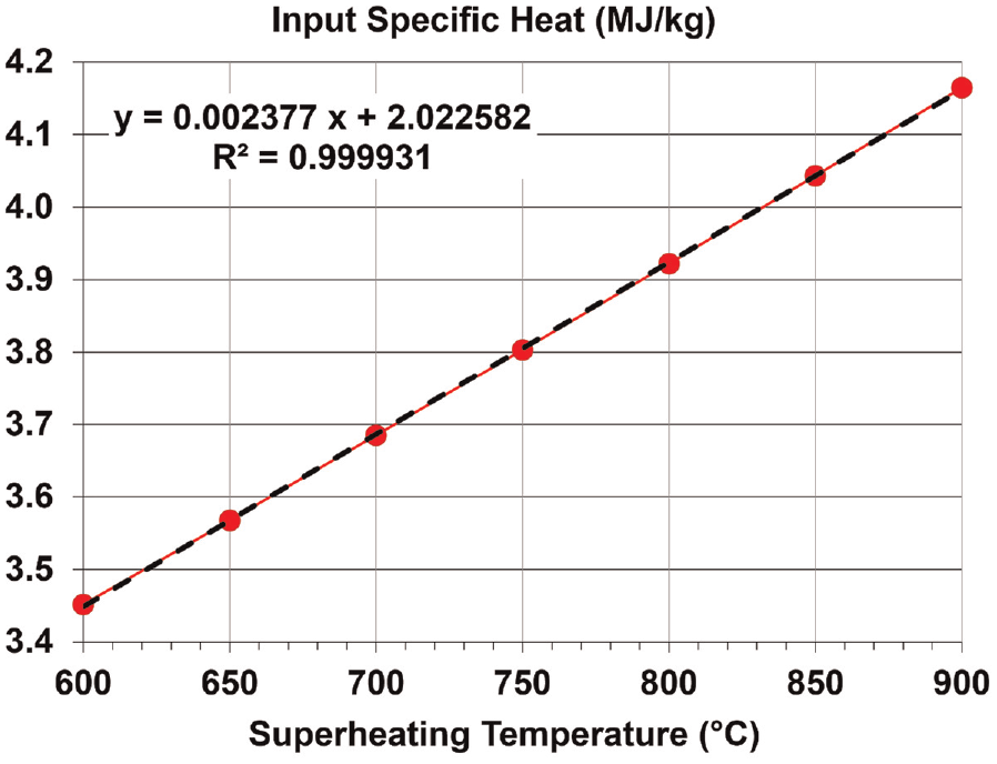
Response of the specific input heat to the superheating temperature.

Figure 8 shows the change (as the superheating temperature increases) in the specific net output shaft work from the cycle, and in the estimated specific output electric energy from a hypothetical power plant that utilizes the steam cycle. Both variations reveal approximately liner relation with the superheating temperature, and this relation has a positive slope. The specific net output shaft work varies from 1332.111 kJ/kg (base case, 600°C) to 1818.681 kJ/kg (at 900°C). Therefore, the average temperature sensitivity factor for the specific net output shaft work is 1.622 kJ/kg/°C (which is equivalent to 0.001622 MJ/kg/°C). Combining the linear increase in the specific net output shaft work with the superheating temperature and the linear increase in the specific input heat with the superheating temperature explains the similar linear variation in the cycle efficiency with the superheating temperature, since the cycle efficiency is computed as the ratio between the specific net output shaft work and the specific input heat. The estimated specific output electric work varies from 1198.900 kJ/kg (base case, 600°C) to 1636.813 kJ/kg (at 900°C).

Figure 8.

Response of the specific net output shaft work and the estimated specific output electric work to the superheating temperature.

Figure 9 shows the change (as the superheating temperature increases) in the required mass flow rate of the circulating water in order to operate a hypothetical power plant with an arbitrary electric power capacity of 1 GW. The variation is approximately linear over the range of considered temperatures. Whereas all the previously discussed performance response variables were increasing with the superheating temperature, the required mass flow rate of water is decreasing with the superheating temperature. Despite this apparent discrepancy, this behavior is compatible since less demand for water flow rate matches an improved efficiency and more electric work produced by a unit mass of water. The required water mass flow rate varies from 834.10 kg/s (base case, 600°C) to 610.94 kg/s (at 900°C). This means that the average temperature sensitivity factor for the water mass flow rate is −0.7425 kg/s/°C.

Figure 9.

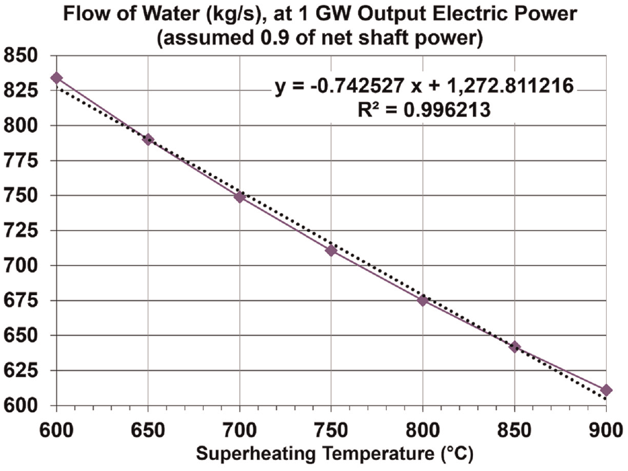
Response of the required water mass flow rate (for operating a 1 GW steam power plant) to the superheating temperature.

Performance with increasing boiler pressure

This subsection is dedicated for presenting the change in the five performance response variables due to increasing the superheated steam pressure beyond the base value of 400 bara. Each response variable is presented in a separate plot. For each response variable, a regression model is added in the plot, including the R-squared value as a measure of the goodness of fit. When selecting a fitting curve, a simpler one (such as linear) is attempted before a more-complicated one (such as quadratic or cubic). A higher-order fitting curve is not attempted if a lower-order fitting is found to be satisfactory. Except for the specific input heat, nonlinear regression models were necessary for good fitting of the data points. The R² value in the case of nonlinear regression does not have its full interpretation (in terms of explaining the variance in the response variable) and usefulness as in the case of the linear regression.⁵⁶ However, it can still be utilized cautiously as an indication of the ability of the regression model to reproduce the discrete data points.^57,58

Figure 10 shows the change in the cycle efficiency and the change in the estimated power plant efficiency as the absolute boiler pressure increases. The variation of either efficiency with the pressure nearly follows a cubic function. The cycle efficiency varies from 38.60% (base case, 50 bara) to 44.60% (at 400 bara). This means an increase by 6.00 percentage points. For the estimated power plant efficiency, the increase is from 34.74% (at 50 bara) to 40.14% (at 400 bara). The nonlinear variation indicates rapid increase with the pressure initially, which declines as the pressure increases further. In particular, the increase in the cycle thermal efficiency between 350 bara and 400 bara is only 0.15 percentage points, whereas the increase in the cycle thermal efficiency between 50 bara and 100 bara is 2.55 percentage points.

Figure 10.

Response of the cycle efficiency and the estimated power plant efficiency to the absolute boiler pressure.

Figure 11 shows the change in the steam quality (dryness fraction) at the turbine exit after the expansion process as the absolute boiler pressure increases. The variation nearly resembles a quadratic function, where the quality decreases as the absolute boiler pressure increases. The steam quality varies from 89.00% (base case, 50 bara) to 72.11% (at 400 bara). This is an adverse effect of elevating the boiler pressure, because it means more erosion in the last part of the steam turbine due to high-speed collisions with the formed liquid droplets. In particular, such low-quality values render the analyzed steam cycle designs for all the pressures above the base case inappropriate practically. One way to solve this problem and bring the turbine exit quality back to a reasonably-high value is raising the superheating temperature. Another remedy is applying reheat modification, where a modified version of the basic Rankine steam cycle is implemented such that the steam is expanded in an initial turbine (high pressure turbine) to intermediate pressure and temperature levels before any condensation occurs. The expanded steam is then heated to become superheated steam again (but at the intermediate pressure level), and is then sent to a subsequent turbine (low pressure turbine), where the reheat steam is expanded to the low-pressure limit before it goes to the condenser. Such reheat modification helps in increasing the turbine-exit steam quality at the expense of increasing the complexity of the cycle.^59,60

Figure 11.

Response of the steam quality at turbine exit to the absolute boiler pressure.

Figure 12 shows the change in the specific heat added to the water as the absolute boiler pressure increases. This response variable is the only one that has a linear variation profile, and it decreases as the boiler pressure increases. This means less heat energy is needed to bring the compressed liquid water to a state of superheated steam at 600°C when this water is more pressurized. This can be explained by the reduced specific enthalpy at state 3 when the pressure at this state increases (while keeping the temperature fixed at 600°C), while the specific enthalpy at state 2 increases as the pressure increases (while keeping its specific entropy fixed). Therefore, the difference in the specific enthalpy of water after the heat addition process (state 3) and before the heat addition process (state 2) decreases as the boiler pressure increases. This means less input heat is needed to achieve the change in the water states from state 2 to state 3. For example, when the boiler pressure increases from 100 bara to 150 bara, the specific enthalpy at state 2 increases from 220.44 kJ/kg to 225.47 kJ/kg, while the specific enthalpy at state 3 decreases from 3625.8 kJ/kg to 3583.1 kJ/kg, thus the specific enthalpy gap drops from 3405.36 kJ/kg to 3357.63 kJ/kg. The specific input heat varies from 3451.410 kJ/kg (base case, 50 bara) to 3099.9 kJ/kg (at 400 bara), with the average rate of decline being 1.006 kJ/kg/bar.

Figure 12.

Response of the specific input heat to the absolute boiler pressure.

Figure 13 shows the change (as the absolute boiler pressure increases) in the specific net output shaft work from the cycle, and the estimated specific output electric work (energy) from a hypothetical power plant that utilizes the steam cycle. Both variations have a cubic relation with the absolute boiler pressure. The specific net output shaft work first increases nonlinearly from 1332.111 kJ/kg (base case, 50 bara) to 1432.67 kJ/kg (at 200 bara), and then decreases nonlinearly to 1382.69 kJ/kg (at 400 bara). Likewise, the estimated specific output electric work first increases nonlinearly from 1198.900 kJ/kg (base case, 50 bara) to 1289.403 kJ/kg (at 200 bara), and then decreases nonlinearly to 1244.421 kJ/kg (at 400 bara). By taking the derivative of the obtained cubic regression model for the specific net output shaft work, and solving for its root located within the pressure range studied here, a point of maximum (optimum) net output work is found at 203 bara, which lies in the subcritical regime. Combining the mound-shaped profile for the specific net output shaft work as a response variable for the boiler pressure as a control variable and the linear decrease in specific input heat as another response variable for the boiler pressure explains the observed asymptotic behavior for the cycle efficiency, which appears to approach a limiting value near 45% if the absolute boiler pressure is increased beyond 400 bara.

Figure 13.

Response of the specific output net shaft work and the estimated specific output electric work to the absolute boiler pressure.

Figure 14 shows the change (as the absolute boiler pressure increases) in the required mass flow rate of the circulating water in order to operate a hypothetical power plant with an arbitrary electric power capacity of 1 GW. Consistent with the mound-shaped profile for the specific net electric output work, the variation profile for the required mass flow rate as a response variable has a valley-shaped curve with a single minimum at an optimum pressure value. This is because the specific net electric output work is inversely proportional to the required mass flow rate (under a fixed target output electric power). Therefore, their profiles should have opposite behaviors. The minimum (optimum) point of the cubic regression model for the needed mass flow rate lies at an absolute boiler pressure value of 203 bara, which is the same optimum pressure value for the maximum net output work. The required water mass flow rate first decreases nonlinearly from 834.10 kg/s (base case, 50 bara) to 775.55 kg/s (at 200 bara), and then increases nonlinearly to 803.59 kg/s (at 400 bara).

Figure 14.

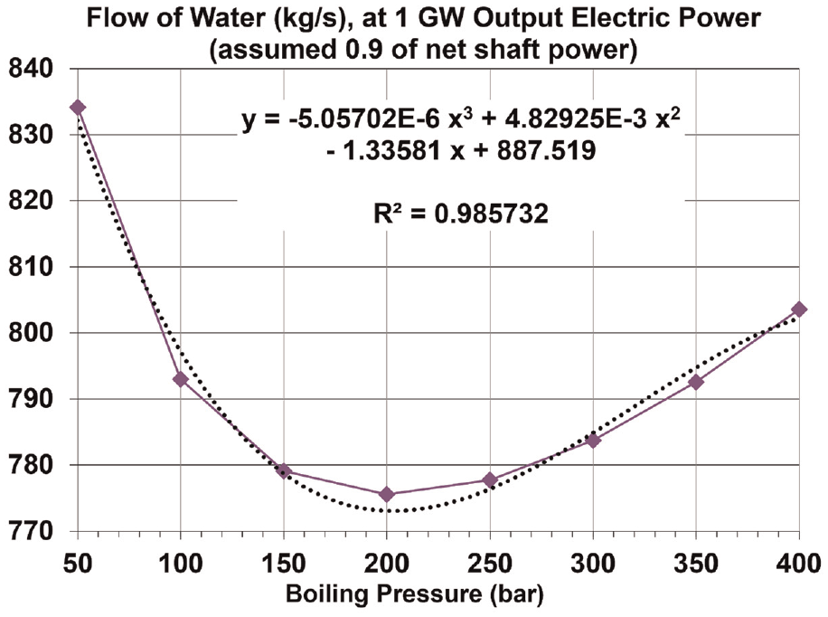
Response of the required water mass flow rate (for operating a 1 GW steam power plant) to the absolute boiler pressure.

Discussion

This section provides some remarks about the results already presented earlier. The first remark is that some response variables are dependent. For example, the cycle efficiency can be derived from the specific net output shaft work and the specific input heat.⁶¹ Despite this, the behavior of each response variable can be different. Also, examining the variation profile of individual variables can help in explaining the variation profile of another dependent variable. This was evident when examining the effect of the boiler pressure. Therefore, studying such response variables individually is justified.

The second remark is about the simplification implemented in the analysis. The cycle studied is idealized, with some neglected losses and with four processes only. For example, there are no feed water heaters.⁶² This simplicity in the modeling has the advantage of reducing uncertainties and having more fair assessment. For example, if irreversibility losses were included, additional unknowns appear in the model, such as the turbine isentropic efficiency,⁶³ which is a parameter to be assumed. Therefore, eliminating such arbitrary factors is preferred when possible. The value of this study does not lie in the particular numerical results presented, but in the trends in the performance as the superheated steam condition changes. The qualitative behavior of response variables is demonstrated through representative quantitative results. The simplicity of the used modeling method also makes the results easy to reproduce and validate by others. It also makes this study attractive for inclusion in the content of college courses about thermodynamics or about power plants, where students are exposed to examples of applying thermodynamic principles in power plants.

The third remark is about the practicality of some examined conditions. It is understood that the upper limits of the temperature and pressure ranges examined here may not be realistic given the presently-available materials and economic feasibility of specialized alloys,^64–68 especially for the temperature. Despite this, the predictions made here can still be useful as theoretical expectations. The expected gains presented here in the cycle efficiency, as well as the changes in other response variables, may be inputs to researchers in material science and steam technology to help assess the feasibility of synthesizing specialized alloys or methods to reach tougher operational conditions not available currently.

The fourth remark is about limitations in the current research study. It should be clarified that the mathematical fitting models presented here are not intended to be universally applicable. Instead, they correspond to a certain condenser pressure, as a fixed value. Despite this, the selected value seems reasonable, making the presented results still useful. Another limitation in the current analysis is that it does not include economic aspects, such as the levelized cost of energy (LCoE) and the life cycle cost (LCC)⁶⁹ which are out of the scope of the current work. The work considers performance from the perspective of engineering design, such as the estimated power plant efficiency. For example, the current analysis can provide an answer to the question: which change is expected to cause more electricity generation for a steam-based power plant with a similar configuration to the one studied here, increasing the peak steam temperature from 600°C to 650°C, or increasing the peak steam pressure from 50 bara to 100 bara? The answer can be made based on the found results that increasing the peak steam pressure from 50 bara to 100 bara is preferred as the power plant efficiency is then expected to increase from 34.74% to 37.03%, whereas increasing the peak steam temperature from 600°C to 650°C is expected to cause the power plant efficiency to increase from 34.74% to 35%⁴⁸. However, the current study cannot answer a question like: which change costs more in retrofitting a steam-based power plant with a similar configuration to the one studied here, increasing the peak steam temperature from 600°C to 650°C, or increasing the peak steam pressure from 50 bara to 100 bara?

The fifth remark is about the value of the presented study and results. The study provides analytical description of how important performance variables in an idealized steam power cycle change with the peak temperature, up to 900°C. The study provides analytical description of how important performance variables in an idealized steam power cycle change with the peak steam pressure, up to 400 bara, covering both subcritical and supercritical regimes of steam. The study gives quantitative illustration of the nonlinear dependence of the cycle efficiency on the peak pressure, which alarms designers of such thermodynamic power cycles that special care is needed when selecting the peak steam pressure. This is unlike the peak steam temperature, where the study suggests that it can be set to the highest possible value (depending on what the involved equipment tolerates) for better utilization of the steam-based power plant. The study includes validation for two different free tools for computing steam properties (Spirax Sarco calculator, and mini-REFPROP), showing agreement between them. The study also showed agreement between these two tools and a third free tool for computing steam properties (Cantera) as analyzing steam cycles, although it was not used directly in the current study.

Conclusions

Considering a four-process, four-device Rankine steam cycle, the effect of the superheated steam temperature (superheating temperature) and the effect of the superheated steam pressure (boiler pressure) were examined. The superheating temperature was varied from 600°C to 900°C, while keeping the absolute boiler pressure fixed at a base value of 50 bara. The absolute boiler pressure was varied from 50 bara to 400 bara, while keeping the superheating temperature fixed at a base value of 600°C, thus both subcritical and supercritical regimes were covered. The condenser pressure was fixed at a reasonable value of 0.125 bara.

Increasing the superheating temperature as a control variable (while keeping the boiler pressure constant) leads to linear improvements in the cycle thermal efficiency, the turbine-exit steam quality, the specific net output shaft work, and the required mass flow rate of water (to achieve a given electric power capacity). The thermal efficiency increases from 38.60% at 600°C to 43.67% at 900°C. This encourages research in specialized metal alloys and techniques that can sustain operating at such elevated temperatures, while making such operation feasible economically.

Increasing the boiler pressure as a control variable (while keeping the superheating temperature constant) shows different effects on the cycle performance. The cycle thermal efficiency appears to have an upper limit near 45%, with further increases in pressure do not yield remarkable improvements. The thermal cycle efficiency increases from 38.60% at 50 bara to 43.30% at 200 bara, and then to 44.60% at 400 bara. This suggests that keeping the absolute boiler pressure near 200 bara may be a reasonable choice. This is a high-pressure condition but still within the subcritical regime, although it is close to the supercritical regime. The idea of increasing the boiler pressure alone is not practical due to the reduced steam quality at the turbine exit, which becomes well below 88%. An optimum pressure point of 203 bara is found for the specific output work (either net shaft work or electric work) and the needed mass flow rate of water (for a specified target electric power capacity).

When a conversion efficiency (defined as the electric power output divided by the mechanical net output shaft power) is taken as 90%, this study concludes that 834.10 kg/s flow rate of recirculating water/steam is needed at the base case of 600°C peak steam temperature and 50 bara peak steam pressure, in order to achieve an electric power generation capacity of 1 GW. This water demand can decrease to 610.94 kg/s if the peak steam temperature can be increased to 900°C. Instead, it is concluded that another way to reduce the demanded water is increasing the peak steam pressure to about 200 bara, where the required mass flow rate of water per 1 GW of electric power output is 775.55 kg/s. This further concludes that the steam temperature is a more-effective design variable than the steam pressure.

In the current work, the peak steam temperature (turbine inlet temperature), and the peak steam pressure were varied in isolation from each other. This means that when one variable is altered, the other remains fixed. This approach enabled better manifestation of the influence of each variable alone. As a possible way to extend the current study, a two-dimensional map of performance variables can be made, where both variables are allowed to change together. This may enable reaching better optimized operating conditions.

Some key conclusions from the current research study are summarized below:

Increasing the peak steam pressure in a simple Rankine steam cycle has a gradually-decreasing gain in terms of the cycle efficiency.

Increasing the peak steam pressure in a simple Rankine steam cycle results in less specific input heat, but results in a mound-shaped profile for the specific net output shaft work.

Increasing the peak steam temperature in a simple Rankine steam cycle has a linearly-increasing gain in terms of the cycle efficiency.

Increasing the peak steam temperature in a simple Rankine steam cycle results in a linearly-increasing profile of the specific input heat as well as the specific net output shaft work.

The steam calculation tools (Spirax Sarco calculator, and mini-REFPROP program) seem to be very consistent.

The Python package Cantera seems to be very capable of modeling steam power cycles.

Research in the field of materials is encouraged, such that steam turbines can sustain ultra-hot steam near 1000°C to realize potential gains in steam-based power plants.

Footnotes

Appendix

Handling Editor: Chenhui Liang

Author contributions (author statement)

Osama A. Marzouk: Conceptualization, Methodology, Software, Formal analysis, Investigation, Writing – Original Draft, Writing – Review & Editing, Visualization.

Declaration of conflicting interests

The author declared no potential conflicts of interest with respect to the research, authorship, and/or publication of this article.

Funding

The author received no financial support for the research, authorship, and/or publication of this article.

ORCID iD

Osama A. Marzouk

Data availability statement

No dataset was used. The results reflect self-generated data, through using free-to-use offline or online software applications, as described in the text with proper citation and references.

References

IRENA [International Renewable Energy Agency]. World Energy Transitions Outlook 2022 - Chapter 1: A roadmap to 2030, https://www.irena.org/Digital-Report/World-Energy-Transitions-Outlook-2022#page-2 (2022, accessed 29 November 2022).

EC [European Commission]. Renewable energy targets, https://energy.ec.europa.eu/topics/renewable-energy/renewable-energy-directive-targets-and-rules/renewable-energy-targets_en (2022, accessed 29 November 2022).

EIA [United States Energy Information Administration]. Electricity explained - Electricity in the United States, https://www.eia.gov/energyexplained/electricity/electricity-in-the-us.php (2023, accessed 5 August 2023).

Farhan

Salem

Ismael

, et al. Impact of suction line on evaporator effectiveness in refrigeration cycle. Case Stud Therm Eng 2021; 27: 101270. DOI: 0.1016/j.csite.2021.101270.

Ameen

ASH

Sinjari

. Design and implementation of evaporative cooler automation system at Erbil/perdawd power plant. Tikrit J Eng Sci 2022; 29: 1–14.

Zhu

Wen

Wang

, et al. Numerical Calculation of Ultrasonic Signal Propagation Characteristics in Steam System of Nuclear Power Plant. In: Proceedings of the 2022 29th International Conference on Nuclear Engineering, Virtual, 8–12 August 2022, paper no. ICONE29-92107. DOI: 10.1115/ICONE29-92107.

Jouhara

. Waste heat recovery in process industries. Weinheim, Germany: John Wiley Sons, 2022.

Sreejith

Prashant

Benny

, et al. Preparation of biological samples for SEM: techniques and procedures. In: Kamaraj

Thirumurugan

Dhanabalan

, et al. (eds) Microscopic techniques for the non-expert. Cham: Springer, 2022, pp. 227–241. DOI: 10.1007/978-3-030-99542-3_10.

Ferreira

Molnar Jazić

Gouveia

, et al. Valorisation of microalga Tetradesmus obliquus grown in brewery wastewater using subcritical water extraction towards zero waste. Chem Eng J 2022; 437: 135324. DOI: 10.1016/j.cej.2022.135324.

10.

Ishikawa

Ozawa

Saito

, et al. Analysis of localized oxides and oxide films formed on alloy 625 and 617 in supercritical water and superheated steam environments at 750°C. Mech Eng J 2017; 4: 17. DOI: 10.1299/mej.17-00013.

11.

Anisimov

. Cold and supercooled water: A novel supercritical-fluid solvent. Russ J Phys Chem B 2012; 6: 861–867. DOI: 10.1134/S199079311208009X.

12.

Chowdhury

Ehsan

. A critical overview of working fluids in organic rankine, supercritical Rankine, and supercritical Brayton cycles under various heat grade sources. Int J Thermofluids 2023; 20: 100426. DOI: 10.1016/j.ijft.2023.100426.

13.

Long

III Wang

. Development and analysis of an integrated mild/partial gasification combined cycle. J Energy Resour Technol 2022; 144: 122102. DOI: 10.1115/1.4054189.

14.

Dincer

Bicer

. Chapter 2 - Fundamentals of energy systems. In: Dincer

Bicer

(eds) Integrated energy systems for multigeneration. Amsterdam, Netherlands: Elsevier Science, 2020, pp. 33–83. DOI: 10.1016/B978-0-12-809943-8.00002-9.

15.

Aljundi

. Energy and exergy analysis of a steam power plant in Jordan. Appl Therm Eng 2009; 29: 324–328.

16.

Shen

, et al. Steam power plant configuration, design, and control. WIREs Energy Environ 2015; 4: 537–563. DOI: 10.1002/wene.161.

17.

Rosen

. Energy- and exergy-based comparison of coal-fired and nuclear steam power plants. Exergy Int J 2001; 1: 180–192. DOI: 10.1016/S1164-0235(01)00024-3.

18.

Wang

Yan

Wang

, et al. Parametric optimization of steam cycle in PWR nuclear power plant using improved genetic-simplex algorithm. Appl Therm Eng 2017; 125: 830–845. DOI: 10.1016/j.applthermaleng.2017.07.045.

19.

Gebreegziabher

Oyedun

Luk

, et al. Design and optimization of biomass power plant. Chem Eng Res Des 2014; 92: 1412–1427. DOI: 10.1016/j.cherd.2014.04.013.

20.

Zarza

Rojas

González

, et al. INDITEP: the first pre-commercial DSG solar power plant. Sol Energy 2006; 80: 1270–1276. DOI: 10.1016/j.solener.2005.04.019.

21.

d’Entremont

Corgnale

Hardy

, et al. Simulation of high temperature thermal energy storage system based on coupled metal hydrides for solar driven steam power plants. Int J Hydrogen Energy 2018; 43: 817–830. DOI: 10.1016/j.ijhydene.2017.11.100.

22.

Matjanov

Akhrorkhujaeva

. Solar repowering existing steam cycle power plants. Int J Thermofluids 2023; 17: 100285. DOI: 10.1016/j.ijft.2023.100285.

23.

Khaleel

Ibrahim

Ismail

, et al. Modeling and analysis of optimal performance of a coal-fired power plant based on exergy evaluation. Energy Rep 2022; 8: 2179–2199. DOI: 10.1016/j.egyr.2022.01.072.

24.

Khaleel

Ismail

Ibrahim

. Parametric assessment of the thermal performance of coal-fired Power Plant. J Adv Res Fluid Mech Therm Sci 2021; 87: 27–43. DOI: 10.37934/arfmts.87.2.2743.

25.

F-Chart Software, LLC. EES: Engineering Equation Solver, https://fchartsoftware.com/ees (2023, accessed 5 August 2023).

26.

Khaleel

Ismail

Ibrahim

. Energy and exergy assessment of the coal-fired power plant based on the effect of condenser pressure. J Mech Eng Res Dev 2021; 44: 69–77.

27.

Piwowarski

. Optimization of steam cycles with respect to supercritical parameters. Pol Marit Res 2009; 16: 45–51.

28.

Zaryankin

Lyskov

Arianov

, et al. Super powerful steam superheaters and turbines for hybrid nuclear power plants. J Power Technol 2011; 91: 45–51.

29.

Siemens Energy. Utility Steam turbines from 90 to 1,900 MW [Brochure], https://assets.siemens-energy.com/siemens/assets/api/uuid:3f7c56be-ba69-4de8-8d2d-ee1febcc7fb1/se-brochure-utility-steam-turbines-220112.pdf (2021, accessed 30 August 2023).

30.

Napier

Dunn

. Chapter 13 - Production of electrical power. In: Dryden

IGC

(ed.) The efficient use of Energy, 2nd ed. Beccles, UK: Butterworth-Heinemann, 1982, pp. 286–308. DOI: 10.1016/B978-0-408-01250-8.50022-2.

31.

Tramošljika

Blecich

Bonefačić

, et al. Advanced ultra-supercritical coal-fired power plant with post-combustion carbon capture: analysis of electricity penalty and CO₂ emission reduction. Sustainability 2021; 13: 801. DOI: 10.3390/su13020801.

32.

DiPippo

. 9 - Elements of thermodynamics, fluid mechanics, and heat transfer applied to geothermal energy conversion systems. In: DiPippo

(ed.) Geothermal power generation - developments and innovation. Duxford, UK: Woodhead Publishing, 2016, pp. 217–247. DOI: 10.1016/B978-0-08-100337-4.00009-7.

33.

Marzouk

Arman

Saadi

MMA

, et al. Thermal power plant with 1 GW capacity for meeting future national electric demands. J Power Energy Eng 2022; 10: 1–11. DOI: 10.4236/jpee.2022.108001.

34.

Khalaf

Mohammed

. An experimental investigation on heat transfer enhancement in an annulus with rotating outer cylinder using nano fluids. Tikrit J Eng Sci 2022; 29: 51–60. DOI: 10.25130/tjes.29.2.7.

35.

Spirax Sarco Limited. Steam Table Calculator, https://www.spiraxsarco.com/resources-and-design-tools/steam-tables/sub-saturated-water-region (2022, accessed 30 November 2022).

36.

NIST [United States National Institute of Standards and Technology]. mini-REFPROP - Version 10.0, https://trc.nist.gov/refprop/MINIREF/MINIREF.HTM (2020, accessed 30 November 2022).

37.

Ilieva

; University of Beira Interior. Mechanisms of water droplets deposition on turbine blade surfaces and erosion wear effects. J Appl Fluid Mech 2017; 10: 551–567. DOI: 10.18869/acadpub.jafm.73.239.26208.

38.

Fan

Wang

Yao

, et al. Research on water droplet movement characteristics in the last two stages of low-pressure cylinder of steam turbine under low load conditions. Front Energy Res 2021; 9: 798305. DOI: 10.3389/fenrg.2021.798305.

39.

Sarkar

. Thermal power plant - design and operation. Amsterdam, Netherlands: Elsevier, 2015. DOI: 10.1016/C2014-0-00536-9.

40.

Reddy

Nanda

Dalai

, et al. Supercritical water gasification of biomass for hydrogen production. Int J Hydrogen Energy 2014; 39: 6912–6926. DOI: 10.1016/j.ijhydene.2014.02.125.

41.

Bischoff

Rosenbauer

Pitzer

. The system NaCl-H₂O: relations of vapor-liquid near the critical temperature of water and of vapor-liquid-halite from 300° to 500°C. Geochim Cosmochim Acta 1986; 50: 1437–1444. DOI: 10.1016/0016-7037(86)90317-0.

42.

Pei

, et al. Examination of the expander leaving loss in variable organic Rankine cycle operation. Energy Convers Manag 2013; 65: 66–74. DOI: 10.1016/j.enconman.2012.06.023.

43.

Mehrpooya

Dehghani

Ali Moosavian

. Optimal design of solid oxide fuel cell, ammonia-water single effect absorption cycle and Rankine steam cycle hybrid system. J Power Sources 2016; 306: 107–123. DOI: 10.1016/j.jpowsour.2015.11.103.

44.

Özgür

. Performance, emission, energetic and exergetic analyses of a compression ignition engine fuelled with sunflower oil methyl esters. Int J Autom Eng Technol 2019; 8: 70–75. DOI: 10.18245/ijaet.524745.

45.

Khaleel

Ibrahim

Ismail

. Thermal performance of coal-fired power plant based on number of feedwater heaters. J Adv Res Fluid Mech Therm Sci 2022; 95: 188–205. DOI: 10.37934/arfmts.95.1.188205.

46.

Marzouk

Al Kamzari

Al-Hatmi

, et al. Energy Analyses for a Steam Power Plant Operating under the Rankine Cycle. In: Proceedings of the First International Conference on Engineering, Applied Sciences and Management (UoB-IEASMA 2021) (ed Al Kalbani

Kanna

Rabai

LB EP

Ahmad

Valsala

), Virtual, 28–29 March 2021, paper no. UOB-IEASMA-102, pp. 11–22. India: IEASMA Consultants LLP. DOI: 10.5281/zenodo.4647963

47.

Zaidan

Ibrahim

Alkumait

AAR

. Performance enhancement by using wet pad in vapor compression cooling system. J Power Sources 2019; 51: 48–63. DOI: 10.5614/j.eng.technol.sci.2019.51.1.4.

48.

Khaleel

Basim Ismail

Khalil Ibrahim

, et al. Energy and exergy analysis of the steam power plants: A comprehensive review on the classification, development, improvements, and configurations. Ain Shams Eng J 2022; 13: 101640. DOI: 10.1016/j.asej.2021.11.009.

49.

Khaleel

Ibrahim

Ismail

, et al. Developing an analytical model to predict the energy and exergy based performances of a coal-fired thermal power plant. Case Stud Therm Eng 2021; 28: 101519. DOI: 10.1016/j.csite.2021.101519.

50.

Struchtrup

. Thermodynamics and energy conversion. Berlin & Heidelberg, Germany: Springer-Verlag, 2014. DOI: 10.1007/978-3-662-43715-5.

51.

Komarudin

Abrianto

Multi

, et al. Performance analysis of extraction condensing turbine - unit 1 at Pltu X, Bekasi, West Java. Int J Adv Multidiscip Res 2023; 2: 130–138.

52.

Marzouk

; College of Engineering, University of Buraimi, Al Buraimi, Postal Code 512, Sultanate of Oman. Cantera-based Python computer program for solving steam power cycles with superheating. J Emerg Technol Adv Eng 2023; 13: 63–73. DOI: 10.46338/ijetae0323_06.

53.

Goodwin

Moffat

Schoegl

, et al. Cantera: An Object-oriented Software Toolkit for Chemical Kinetics, Thermodynamics, and Transport Processes (2.6.0). Zenodo, https://doi.org/10.5281/zenodo.6387882 (2022, accessed 5 August 2023).

54.

Cantera Developers. The Cantera Community, https://www.cantera.org (2023, accessed 5 August 2023).

55.

Miles

. R-squared, adjusted R-squared. In: Everitt

Howell

(eds) Encyclopedia of statistics in behavioral science. Wiley, 2005. DOI: 10.1002/0470013192.bsa526.

56.

Spiess

Neumeyer

. An evaluation of R² as an inadequate measure for nonlinear models in pharmacological and biochemical research: a Monte Carlo approach. BMC Pharmacol 2010; 10: 6. DOI: 10.1186/1471-2210-10-6.

57.

Chicco

Warrens

Jurman

. The coefficient of determination R-squared is more informative than SMAPE, MAE, MAPE, MSE and RMSE in regression analysis evaluation. PeerJ Comput Sci 2021; 7: e623. DOI: 10.7717/peerj-cs.623.

58.

Onofri

. The R-squared and nonlinear regression: a difficult marriage?, https://www.statforbiology.com/2021/stat_nls_r2 (2021, accessed 2 December 2022).

59.

Dechamps

. Advanced Combined Cycle Alternatives with the latest gas turbines. ASME J Eng Gas Turbine Power 1998; 120: 350–357. DOI: 10.1115/1.2818129.

60.

Salazar-Pereyra

Lugo-Leyte

Bonilla-Blancas

, et al. Thermodynamic Analysis of Supercritical and Subcritical Rankine Cycles. In: Proceedings of the ASME Turbo Expo 2016: Turbomachinery Technical Conference and Exposition. Volume 8: Microturbines, Turbochargers and Small Turbomachines; Steam Turbines, Seoul, South Korea, 13–17 June 2016, paper no. GT2016-57814. DOI: 10.1115/GT2016-57814

61.

Ahmed

Ayub

Sheikh

, et al. Thermodynamic optimization and performance study of supercritical CO₂ thermodynamic power cycles with dry cooling using response surface method. Int Commun Heat Mass Transf 2023; 142: 106675. DOI: 10.1016/j.icheatmasstransfer.2023.106675.

62.

Mohammed

Al Doori

Jassim

, et al. Energy and exergy analysis of the steam power plant based on effect the numbers of feed water heater. J Adv Res Fluid Mech Therm Sci 2020; 56: 211–222.

63.

Medina-Flores

Picón-Núñez

. Modelling the power production of single and multiple extraction steam turbines. Chem Eng Sci 2010; 65: 2811–2820. DOI: 10.1016/j.ces.2010.01.016.

64.

Viswanathan

Coleman

Rao

. Materials for ultra-supercritical coal-fired power plant boilers. Int J Press Vessel Piping 2006; 83: 778–783. DOI: 10.1016/j.ijpvp.2006.08.006.

65.

Shvarts

Verbovetsky

Somova

, et al. Development of technical solutions on a coal-fired boiler for a power plant unit of 800 MW with steam parameters of 35 MPa and 700/720°C. Therm Eng 2015; 62: 892–896. DOI: 10.1134/S0040601515120083.

66.

Ohji

Haraguchi

. 2 - Steam turbine cycles and cycle design optimization: The Rankine cycle, thermal power cycles, and IGCC power plants. In: Tanuma

(ed.) Advances in steam turbines for modern power plants. Duxford, UK: Woodhead Publishing, 2017, pp. 11–40. DOI: 10.1016/B978-0-08-100314-5.00002-6.

67.

Kler

Zharkov

Epishkin

. Parametric optimization of supercritical power plants using gradient methods. Energy 2019; 189: 116230. DOI: 10.1016/j.energy.2019.116230.

68.

GE Steam Power. Advanced Ultra-Supercritical Technology, https://www.ge.com/steam-power/coal-power-plant/usc-ausc (2022, accessed 2 December 2022).

69.

Mulenga

Kabanshi

Mupeta

, et al. Techno-economic analysis of off-grid PV-diesel power generation system for rural electrification: a case study of Chilubi district in Zambia. Renew Energy 2023; 203: 601–611. DOI: 10.1016/j.renene.2022.12.112.

Subcritical and supercritical Rankine steam cycles,under elevated temperatures up to 900°C and absolute pressures up to 400 bara

Abstract

Keywords

Introduction

Background

Goal of the Study

Article structure

Problem statement and main objective

Research method

Models

Source of water properties

Selection of references

Governing equations

Water states

Energy balance

Results

Base case

Performance with increasing superheating temperature

Performance with increasing boiler pressure

Discussion

Conclusions

Footnotes

Appendix

Author contributions (author statement)

Declaration of conflicting interests

Funding

ORCID iD

Data availability statement

References