Modeling and analysis of static and dynamic behavior of marine towed cable-array system based on the vessel motion

Abstract

Towing cables are playing a key role in maneuverability of moving or submerged vessels and the supporting vehicles in the ocean. This investigation evaluates the tension strength of the various parts of the marine towing cable and its geometric form under various operating conditions. Thus, the governing equations of the problem are introduced and analyzed first, followed by an examination of the method of solving the problem. We evaluate the cable’s static and dynamic behavior under different operating conditions using a continuous cable method. Then, we introduce and analyze the governing equations of the problem. The static mode comprises three operating conditions: a two-dimensional mode for constant vessel length, a two-dimensional mode for constant hydrophone depth, and a three-dimensional mode for different vessel motion and seawater directions. Dynamic mode operating conditions include vessel acceleration, vessel rotation, and cable tightening. The results show that, if the velocity of the seawater flow is zero, changing the angle of the vessel motion has little effect on the tension force of the cable-array and the length of the cable in the steady-state. It is also found that assuming a constant depth of the cable-array, the maximum tension force of the cable will increase to almost 35 times. However, if the length of the cable-array remains constant, the maximum tension force of the cable increases by around 13 times as the vessel’s speed increases by 5 times.

Introduction

Towing cables are frequently used in the ocean environment and play a key role in supplying power and correspondence among moving or submerged vessels and the supporting vessel. ¹ Nevertheless, the operation and connection of the towing cable and the drag relative to the flow of water limit the maneuverability of these vehicles. Thus, measuring the resulting impact generated by the towing cable and the flow would help assess the vehicle’s maneuvering behavior. ² Many scientists are neglecting the impact of the towing cable since its effect would make the computational model quite complex and impossible to solve. Ergo, just a handful of researchers address these problems by including the consequences of the towing cable. Various methods with various properties exist for this purpose: experimental testing, Finite Element Methods (FEM), Finite Difference Methods (FDM), Catenary Equations, Lump-Mass-Spring Formulation (LMS), and Finite Segment Methods (FSA).

The dynamic tensions and deflections caused by surface vessel movements in heavy weather frequently restrict the design of a towed underwater system. A towed system’s huge curvatures and quadratic fluid drag require either a long simulation or an approximation analysis. Small perturbations and similar linearization are two typical simplifications. Dynamic deflections are defined in the first as tiny movements from a known static configuration.^3,4 By retaining just first-order terms, the geometric coupling terms become linear. Because static cable curvatures could be fairly big, but wave-induced movements are rather small, perturbation theory works particularly well for ocean systems. An equivalent linearization is indeed a basic approach in nonlinear mechanics; fluid drag linearization has been frequently employed in ocean situations, allowing approximate frequency-domain analysis.

Bliek ⁵ proposed a matrix technique for mooring system analysis based on these simplifications. This approach employs an iterative loop and transfer matrices derived from a finite-difference decomposition of the cable equations to adjust the linearization. Buckham et al. ⁶ used the FEM to quantify the strain and bending force on the slack cord connected to the remotely operated vehicle (ROV). The computational load of this solution is heavy, and it is complicated to integrate such packs into the design of the control system. Ablow and Schechter ⁷ also suggested an implied FDM simulation of the undersea cables (UC), usually referred to in the related literature. Even so, if the tension in the UC is missed, the formula becomes singular. The structure of the LMS has a straightforward physical interpretation and does not involve a significant amount of computation. Chai et al. ⁸ proposed a novel formula of LMS that permitted a static and dynamic study of many slender structures. Winget and Huston ⁹ explored cable dynamics with the finite segment approach (FSA). They modeled the cables as a set of couplings attached by ball-and-socket connections. While several studies have been performed on the hydrodynamics of the UC structure, they include different limitations.

For example, Franchi et al. ¹⁰ presented a dynamic model based on the autonomous underwater vehicle (AUV) navigation strategy, as confirmed by FeelHippo AUV experimental data. However, a review of the studies in the field of sonar shows that little research has been done on the effect of the fluid flow field on the dynamic behavior of the sonar cable. For example, Vu et al. ¹¹ mathematically modeled complete equations to simulate the behavior of a vehicle under the influence of cable movement in a coastal sea in the rigid motion of the subsurface and the flexible motion of a central cable. To model the cable behavior, they used catenary equations along with the shooting method to solve the problem of two-point boundary conditions. They showed that the movement of the cable influences the movement of the body carrying it. González et al. ¹² investigated the effect of the material of the vessel cable on its dynamic behavior. They used a spring-based model and a multi-body model to simulate the cable. Their research revealed that both models might be used depending on the application of the problem, as well as the advantages and limits of each strategy. In a numerical study sample, Du et al. ¹³ investigated the effect of the subsurface vehicle flow field and its impeller on the dynamic behavior of a sonar cable. They used the Lumped-Mass method for this simulation. They also used the computational fluid dynamics method to calculate the drag forces on the cable. In this research, for simulation, three-movement modes, including linear, torsional, and surface movements for the vehicle, have been considered. Their results showed that the lateral deflections of the cable depended on the velocity and motion of the subsurface vehicle. Using the Lumped-Mass method, Zhu and Yoo ¹⁴ investigated the dynamics of the offshore cable with a new reference framework for the elements obtained by the element direction vector and the relative fluid velocity. After comparison with other methods, they showed that this method is suitable for dynamic analysis of vessel cable behavior.

Kebede et al. ¹⁵ experimentally compared the hydrodynamic forces acting on a spiral rope with a simple rope as a fishing net holder. Their work studied the effect of rope diameter, flow velocity, and flow attack angle on hydrodynamic forces. The results showed that the spiral rope generates more lift force than the ordinary rope. In numerical dynamic analysis, Shin et al. ¹⁶ obtained the equations of motion for the static, dynamic, and vibrational states for a cable connected to a subsurface vehicle on the other side of which drogues are installed. Their results showed that increasing the towing velocity increases the tension along the cable in the static state. Biao et al. ¹⁷ modeled the effects of cable tension, rotation radius, and flow on a vessel cable’s dynamic behavior during ship rotation movements. The findings indicate that the cable stretching velocity and rotation radius effectively increase or lessen the V deformation of the cable.

In the past five decades, cable mechanics have been the focus of extensive research. Modern algorithms for analyzing submerged cables make use of a spatial discretization of the cable’s continuous partial differential equations based on the finite element method ¹⁸ or finite differences. ¹⁹ These methods incorporate the influence of geometry and structural nonlinearities, and their robustness permits the simulation of constant-length towing cables with second-scale steps. Hover et al. ²⁰ studied dynamical movements and tensions in towed underwater cables employing a matrix approach for a mooring system in conjunction with equivalent linearization and small perturbation theory, as well as pitching tow fish modeling. Two examples of the technique’s applicability are provided. The initial paper investigates an essential limitation of constrained passive heave compensation, whereas the second investigates the utilization of floated tethers for dynamic decoupling. Srivastava et al. ²¹ estimated the dynamic behavior of an underwater 3D model of a towed cable in a linear profile using a central finite difference technique in a different mathematical approach. Their devised numerical program is applicable to towed array systems for detecting a submarine or moving object. Rodrguez Luis et al. ²² computed the marine towing cable dynamics via a finite element approach by minimizing the numerical results’ noise and taking into account the Rayleigh springs model that represents the tension of the line. The proposed model is based on a dynamic analysis of a catenary line traveling between two entities, one with an imposed motion and the other with an unconstrained motion. The findings indicate that cable length could have a crucial role in ship destruction. Adding a floating towed body to the towing line at a point near the towed body might decrease the horizontal tension at the ship’s fairlead, and for both kinds of towed bodies, the dependence of the drag forces on the towing system on ship speed must be taken into account when determining the ideal transport speed.

According to a review of prior studies, researchers have not performed a static-dynamic analysis of the towed cable array with the technique of comparing its functional-application circumstances. The research of this behavior can be altered by assuming a constant length of cable or a constant depth of cable-array. In this study, the static equations for the hypothetical cable-array are solved using MATLAB code, and the centralized mass approach. This study takes into account operating characteristics such as boundary conditions (velocity and direction of vessel and flow), which have a major impact on the parameters of maximum cable tension, maximum distance from the vessel, and depth or length of the vessel cable. In addition, a three-dimensional dynamic solution was conducted in the current work employing the equations of motion and the centralized mass approach. The rest of this paper is organized as follows: Modeling Approach section introduces the modeling approach. In Results section, we present the simulation results. Finally, Conclusion section includes concluding remarks.

Modeling approach

In the present research, the movement model of a marine towed cable-array system will be developed using the following assumptions. The analyzed system is depicted in Figure 1.

• The cable array system is uninterrupted, extensible, and adaptable.

• Axial deformation will not significantly alter the cross-sectional area of the cable-array system.

• The forces operating on the cable-array system are gravity, buoyancy, tensile force, and hydrodynamic force due to the effect of the flow field.

Figure 1.

Schematic representation of the towed cable-array system.

Continuous mass model of the cable-array

The cable-array is seen as a single curvilinear line in order to determine the governing equations of motion for the cable’s motion as a continuum. Let’s designate the unstretched Lagrangian coordinate along the cable-array, as illustrated in Figure 2, as it is measured from the origin to a material point on the cable-array. The origin, which is designated by the notation s  =  0, is selected to fall on a boundary, such as the cable-array’s free end. The other end-point is designated as s  =  L, where L is the length of the cable array when it is not stretched. The unit vectors $e_t$ , $e_n$ , $e_b$ , respectively represent the tangent, normal, and binormal directions of the local coordinate system. The direction that is tangent to the cable-array axis and points in an increasing s is known as the tangential direction. The binormal direction is determined so that the system of vectors is orthogonal and right-handed, and the normal direction is perpendicular to t. The set of rotations known as Euler angles is used to translate the local coordinate ${\left\{\mathit{tnb}\right\}}_{e_t{e}_n{e}_b}$ into the fixed frame ${\left\{\mathit{XYZ}\right\}}_{\mathrm{ijk}}$ . The values of roll, pitch, and yaw angle, namely a rotation about the Z-axis, a rotation about the resultant Y-axis to bring the X-axis, and a rotation about the Z-axis, may be used to form the rotation matrix. It should be emphasized that in the local coordinate system, any arbitrary vector would be written as $\overrightarrow{\eta }={\eta }_1{e}_t+{\eta }_2{e}_n+{\eta }_3{e}_b$ .

$$\begin{array}{c}\left[\begin{array}{c}{\eta }_1\hfill \\ \multicolumn{1}{c}{{\eta }_2}\\ \multicolumn{1}{c}{{\eta }_3}\end{array}\right]=\mathit{R}\left[\begin{array}{c}{\eta }_X\hfill \\ \multicolumn{1}{c}{{\eta }_Y}\\ \multicolumn{1}{c}{{\eta }_Z}\end{array}\right]\hfill \\ \mathit{R}=\left[\begin{array}{ccc}\cos \phi \cos \theta \hfill & \sin \phi \cos \theta \hfill & -\sin \theta \hfill \\ \multicolumn{1}{c}{\cos \phi \sin \theta \sin \psi -\sin \phi \cos \psi }& \sin \phi \sin \theta \sin \psi +\cos \phi \cos \psi \hfill & \cos \theta \sin \psi \hfill \\ \multicolumn{1}{c}{\cos \phi \sin \theta \sin \psi +\sin \phi \sin \psi }& \sin \phi \sin \theta \sin \psi -\cos \phi \cos \psi \hfill & \cos \theta \cos \psi \hfill \end{array}\right]\hfill \end{array}$$

(1)

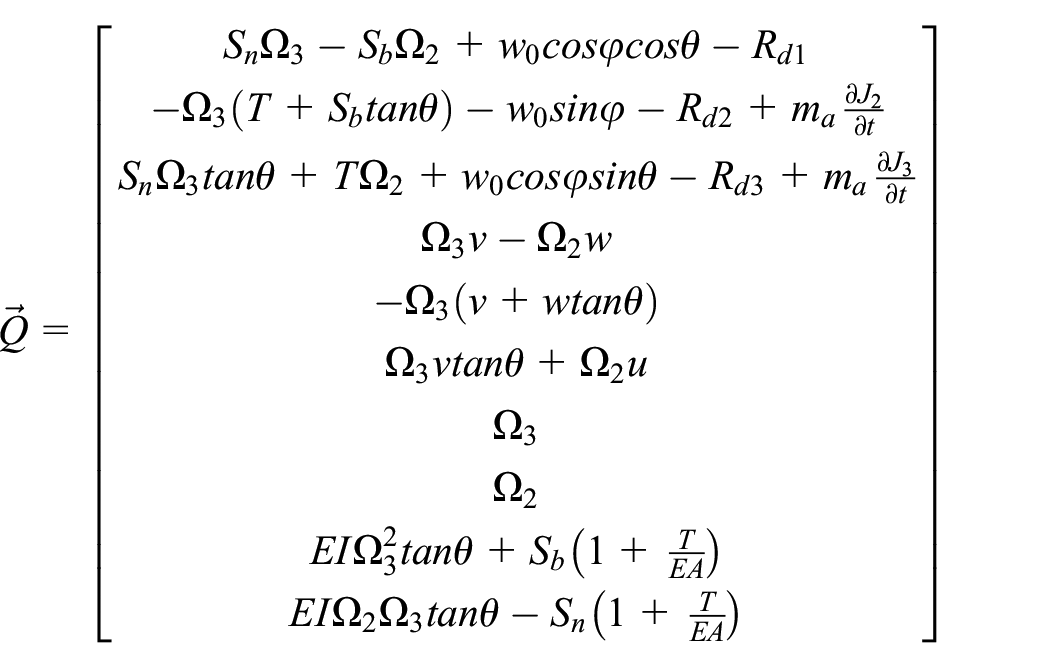
Herein we define the following quantities: circular cross-section A, sectional second moment I, polar moment J, mass per unit length m, density ρ_c, Young’s modulus E, and shear modulus G. The general and three-dimensional dynamic equations could be expressed in matrix form as ²³ :

$$\mathbf{M}\frac{\partial \overrightarrow{Y}}{\partial s}=\mathbf{N}\frac{\partial \overrightarrow{Y}}{\partial t}+\overrightarrow{Q}$$

(2)

where

$$\overrightarrow{Y}={[T_1,T_2,T_3,u,v,w,\phi ,\theta ,{\Omega }_2,{\Omega }_3]}^T$$

(3)

$$\mathbf{M}=\left[\begin{array}{cccccccccc}1\hfill & 0\hfill & 0\hfill & 0\hfill & 0\hfill & 0\hfill & 0\hfill & 0\hfill & 0\hfill & 0\hfill \\ \multicolumn{1}{c}{0}& 1\hfill & 0\hfill & 0\hfill & 0\hfill & 0\hfill & 0\hfill & 0\hfill & 0\hfill & 0\hfill \\ \multicolumn{1}{c}{0}& 0\hfill & 1\hfill & 0\hfill & 0\hfill & 0\hfill & 0\hfill & 0\hfill & 0\hfill & 0\hfill \\ \multicolumn{1}{c}{0}& 0\hfill & 0\hfill & 1\hfill & 0\hfill & 0\hfill & 0\hfill & 0\hfill & 0\hfill & 0\hfill \\ \multicolumn{1}{c}{0}& 0\hfill & 0\hfill & 0\hfill & 1\hfill & 0\hfill & 0\hfill & 0\hfill & 0\hfill & 0\hfill \\ \multicolumn{1}{c}{0}& 0\hfill & 0\hfill & 0\hfill & 0\hfill & 1\hfill & 0\hfill & 0\hfill & 0\hfill & 0\hfill \\ \multicolumn{1}{c}{0}& 0\hfill & 0\hfill & 0\hfill & 0\hfill & 0\hfill & \cos \theta \hfill & 0\hfill & 0\hfill & 0\hfill \\ \multicolumn{1}{c}{0}& 0\hfill & 0\hfill & 0\hfill & 0\hfill & 0\hfill & 0\hfill & 1\hfill & 0\hfill & 0\hfill \\ \multicolumn{1}{c}{0}& 0\hfill & 0\hfill & 0\hfill & 0\hfill & 0\hfill & 0\hfill & 0\hfill & \mathrm{EI}\hfill & 0\hfill \\ \multicolumn{1}{c}{0}& 0\hfill & 0\hfill & 0\hfill & 0\hfill & 0\hfill & 0\hfill & 0\hfill & 0\hfill & \mathrm{EI}\hfill \end{array}\right]$$

$$\begin{array}{c}\mathbf{N}=\hfill \\ \left[\begin{array}{cccccccccc}0\hfill & 0\hfill & 0\hfill & m\hfill & 0\hfill & 0\hfill & -\mathrm{mvcos}\theta \hfill & \mathrm{mw}\hfill & 0\hfill & 0\hfill \\ \multicolumn{1}{c}{0}& 0\hfill & 0\hfill & 0\hfill & m+m_a\hfill & 0\hfill & \mathrm{mucos}\theta +\mathrm{mw}\sin \theta \hfill & 0\hfill & 0\hfill & 0\hfill \\ \multicolumn{1}{c}{0}& 0\hfill & 0\hfill & 0\hfill & 0\hfill & m+m_a\hfill & -\mathrm{mvsin}\theta \hfill & -\mathrm{mu}\hfill & 0\hfill & 0\hfill \\ \multicolumn{1}{c}{\frac{1}{\mathrm{EA}}}& 0\hfill & 0\hfill & 0\hfill & 0\hfill & 0\hfill & 0\hfill & 0\hfill & 0\hfill & 0\hfill \\ \multicolumn{1}{c}{0}& 0\hfill & 0\hfill & 0\hfill & 0\hfill & 0\hfill & (1+\frac{T}{\mathrm{EA}})\cos \theta \hfill & 0\hfill & 0\hfill & 0\hfill \\ \multicolumn{1}{c}{0}& 0\hfill & 0\hfill & 0\hfill & 0\hfill & 0\hfill & 0\hfill & -(1+\frac{T}{\mathrm{EA}})\hfill & 0\hfill & 0\hfill \\ \multicolumn{1}{c}{0}& 0\hfill & 0\hfill & 0\hfill & 0\hfill & 0\hfill & 0\hfill & 0\hfill & 0\hfill & 0\hfill \\ \multicolumn{1}{c}{0}& 0\hfill & 0\hfill & 0\hfill & 0\hfill & 0\hfill & 0\hfill & 0\hfill & 0\hfill & 0\hfill \\ \multicolumn{1}{c}{0}& 0\hfill & 0\hfill & 0\hfill & 0\hfill & 0\hfill & 0\hfill & 0\hfill & 0\hfill & 0\hfill \\ \multicolumn{1}{c}{0}& 0\hfill & 0\hfill & 0\hfill & 0\hfill & 0\hfill & 0\hfill & 0\hfill & 0\hfill & 0\hfill \end{array}\right]\hfill \end{array}$$

$$\begin{array}{c}\multicolumn{1}{c}{\overrightarrow{Q}=\left[\begin{array}{c}{S}_n{\mathrm{\Omega }}_3-S_b{\mathrm{\Omega }}_2+w_0\cos \phi \cos \theta -R_{d1}\hfill \\ \multicolumn{1}{c}{-{\mathrm{\Omega }}_3(T+S_b\tan \theta )-w_0\sin \phi -R_{d2}+m_a\frac{\partial J_2}{\partial t}}\\ \multicolumn{1}{c}{S_n{\mathrm{\Omega }}_3\tan \theta +T{\mathrm{\Omega }}_2+w_0\cos \phi \sin \theta -R_{d3}+m_a\frac{\partial J_3}{\partial t}}\\ \multicolumn{1}{c}{{\mathrm{\Omega }}_{3}v-{\mathrm{\Omega }}_{2}w}\\ \multicolumn{1}{c}{-{\mathrm{\Omega }}_3(v+\mathrm{wtan}\theta )}\\ \multicolumn{1}{c}{{\mathrm{\Omega }}_3\mathrm{vtan}\theta +{\mathrm{\Omega }}_{2}u}\\ \multicolumn{1}{c}{{\mathrm{\Omega }}_3}\\ \multicolumn{1}{c}{{\mathrm{\Omega }}_2}\\ \multicolumn{1}{c}{\mathrm{EI}{\mathrm{\Omega }}_3^2\tan \theta +S_b(1+\frac{T}{\mathrm{EA}})}\\ \multicolumn{1}{c}{\mathrm{EI}{\mathrm{\Omega }}_2{\mathrm{\Omega }}_3\tan \theta -S_n(1+\frac{T}{\mathrm{EA}})}\end{array}\right]}\end{array}$$

Figure. 2.

Coordinate systems and Euler rotation sequence.

In the above equations, T is the tension force of the cable-array, Ω represents the local curvature of the cable-array, m_a is the added mass per unit length and w₀ is submerged cable-array weight per unit length.

In order to solve the governing equations of motion, the cable is first discretized into n nodes, separated by Δs, and time is divided into a series of steps Δt. The set of equations are solved at the mid-point between nodes j and j + 1, denoted by j + 1/2, and at the time i + 1/2. The centered finite difference method is used to express the partial derivatives.

Lumped mass model of the towing cable-array

By simulating the continuity and elasticity of the under consideration towed cable-array system with n massless connections and n lumped-mass points, the cable is represented in this method, as shown in Figure 3. One end of the cable array is free, while the other end could be considered a hinge joint at the stern. The force analysis of the ith section is shown in Figure 2.

Figure 3.

The towed cable-array lumped mass model and force analysis of the ith segment.

The equilibrium equation of forces for the ith segment based on Newton’s second law can be expressed as:

$${\mathit{T}}_i-{\mathit{T}}_{i-1}+{\mathit{W}}_i+{\mathit{F}}_i=m_i{\mathit{a}}_i$$

(4)

where, T is the tension force, F represents the hydrodynamic drag force and W _i represents the force due to weight in water (buoyancy force) and a _i is the acceleration of mass i. The relationship between the tension acting on the ith segment of the cable-array and its coordinates and velocities on either end of the segment can be represented as:

$$T_i=A_i{E}_i(\frac{l_i}{l_{0i}}-1)+{\alpha }_i{A}_i\frac{{\stackrel{·}{l}}_i}{l_{0i}}$$

(5)

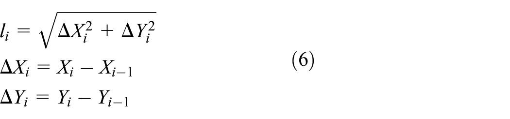
where, A_i is the cross-section, E_i represents the modulus of elasticity, α_i is the damping coefficient, l_0i is the initial length, and l_i is the real length which could be written as

$$\begin{array}{c}{l}_i=\sqrt{\mathrm{\Delta }{X}_i^2+\mathrm{\Delta }{Y}_i^2}\hfill \\ \mathrm{\Delta }{X}_i=X_i-X_{i-1}\hfill \\ \mathrm{\Delta }{Y}_i=Y_i-Y_{i-1}\hfill \end{array}$$

(6)

Equation (4) should be written in the tangential and normal directions separately and the balanced forces will accelerate the element in both directions. Based on the Wilson model, ²⁴ the normal F_n and tangential F_t hydrodynamic drag forces acting on the ith segment are given as follows.

$$F_{\mathrm{ni}}=-\frac{1}{2}{\rho }_0{d}_i{l}_i{C}_{\mathrm{dn}}{V}_{\mathrm{ni}}\left|V_{\mathrm{ni}}\right|$$

(7)

$$F_{\mathrm{ti}}=-\frac{1}{2}{\rho }_0{d}_i{l}_i{C}_{\mathrm{dt}}{V}_{\mathrm{ti}}\left|V_{\mathrm{ti}}\right|$$

(8)

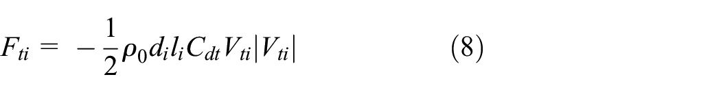
where, ρ₀ is the density of the fluid, d_i is the diameter, C_dn and C_dt are drag coefficients in normal and tangential directions respectively and V_n and V_t are velocity components in normal and tangential directions (C_dn = 1.6 and C_dt = 0.01 in this work).

Results

Comparison of solution methods

According to the results obtained for the two methods, the following remarks are presented from the comparison of the two methods.

• The continuous cable method is suitable for two-dimensional mode, but it has a singular point in three-dimensional mode.

• The continuous cable method has a faster solution procedure compared with the lumped mass method.

• The lumped mass method does not have a singular point problem, but its solution is more time-consuming and requires more calculations, and its static solution is more complicated.

Therefore, for the two-dimensional static mode, the continuous cable method is used, and in the three-dimensional mode, the concentrated mass method is used to check the static and dynamic behavior of the cable.

The characteristics of the cable-array system as well as its operating conditions depend on its application. As a case study, Table 1 represents the physical and structural properties of the considered cable-array system depicted in Figure 1.

Table 1.

Physical and structural characteristics of cable-array system.

Section name	Longitudinal density (kg/m)	Length (m)	Diameter (mm)	Axial rigidity (MN/m)	Structural damping (%)	Vertical drag coefficient (Cdn)	Tangential drag coefficient (Cdt)
Cable	4	200	25	10	0.1	1.6	0.01
First VIM	3.5	30	65	7	0.3	1.6	0.01
Second VIM	3.4	20	65	7	0.3	1.6	0.01
Acoustic array	3.5	40	65	7	0.1	1.6	0.01
Tail	0.206	50	16	0.4	0.1	1.6	0.01

It is necessary to study the number of elements in the output while considering the discretization solution of cable dynamic equations. To reach this aim, the behavior of a cable-array at a vessel velocity of 5 m/s, a constant flow velocity of 0.61 m/s, and a sea depth of 100 m was investigated in two dimensions for a variety of different elements, as shown in Table 2. When the number of total elements was increased tenfold (from 34 to 340), the depth size changed by less than 0.1%, and the maximum tension force changed by around 1.3%, which is negligible. The depth size changed by less than 0.03% as the number of total elements increased (from 68 to 340), and the maximum tension force size increased by around 0.6%, both of which are negligible. Because computation time is critical, 68 total elements appear suitable for calculations (the bold row).

Table 2.

The effects of the number of elements on the results.

Number of towed cable element	Number of first VIM element	Number of the acoustic array element	Number of second VIM element	Number of tail element	Total element	Max tension force (N)	Max depth (m)
20	3	4	2	5	34	6920	44.73
40	6	8	4	10	68	6970	44.70
100	15	20	10	25	170	6999	44.69
200	30	40	20	50	340	7009	44.69

Static behavior

Case 1: Two-dimensional mode of the cable-array with constant length

First, the effect of different velocities of the vessel on the dynamic behavior of the cable-array at a steady state is investigated. The sea water velocity (flow velocity) is considered zero in this case. Figure 4 shows the geometry of the cable-array per constant velocity of the towing vessel. The different parts of the cable-array are arranged in an approximately horizontal straight line to satisfy the assumptions mentioned in the calculation of the equations of motion. It is also known that as the towing velocity decreases, the depth of the cable-array increases. Another finding showed that as the velocity of the towing vessel increases, the maximum distance of the cable-array from the vessel increases.

Figure 4.

Geometric shape of the array in terms of different velocities of the towing vessel.

Figure 5 shows the magnitude of the cable tension force along with the cable-array for different velocities of towing vessels. At less than a velocity of 6 m/s, the increase in tension force in the vessel cable section is less than in the horizontal array section. At a velocity of 6 m/s and higher velocities, the slope of the horizontal arrays is greater. These cases indicate that most of the tension force is due to the vessel cable at low velocities (less than 6 m/s). More tension force is because of the horizontal array section at higher velocities.

Figure 5.

Tension force measurement along the array for different velocities of towing vessel.

Table 3 shows the effect of towing vessel velocity on maximum tension force, depth, and distance from the vessel for the cable-array. As it turns out, as the towing vessel velocity increases, the maximum tension force and the maximum distance from the vessel increase, and the maximum cable-array depth decrease.

Table 3.

Changes in maximum cable tension force, maximum depth, and maximum distance from the vessel for different velocities of towing vessel.

Vessel velocity (m/s)	Max tension (kN)	Max depth (m)	Max distance from vessel (m)
3	4.53	68.84	328.2
6	10.49	33.15	337.4
9	21.96	20.73	339.4
12	38.4	14.45	340.3
15	59.68	10.7	341

Case 2: Two-dimensional mode of the array with constant depth

One of the cable-array’s important operating conditions is the hydrophone array’s placement at a constant depth below sea level. Here, by increasing the vessel velocity and decreasing the angle of the towing cable with the horizon, the length of the towing cable has increased so that the array of hydrophones (where the depth gauge sensor is installed) is located at a certain depth below sea level. In this case, because of the change in the vessel’s length cable, the important parameters of the maximum cable tension, the maximum distance from the vessel, differs greatly from the constant length of the vessel cable. To simulate a cable-array in this situation, the water velocity is assumed to be zero. Figure 6 shows the geometry of the cable-array, and Figure 7 shows the distribution of tension force along with the cable-array for different velocities of towing vessels.

Figure 6.

Geometric shape of the array in terms of different velocities of the vessel for constant depth.

Figure 7.

Tension force measurement along with the cable-array for different velocities of towing vessels at constant array depth.

Table 4 also presents important parameters such as the length of the towing cable, the maximum tension force, and the maximum distance (tail end) of the vessel. The maximum tension force of the cable has increased about 35 times for a 5-fold increase in vessel velocity (from 3 to 15 m/s). The length of the cable-array also increased 5 times. However, it should be considered that at low velocities (less than 6 m/s), the distance of the acoustic array from the vessel will be less than 300 m, which may negatively affect the reception of waves from other vessels.

Table 4.

Changes in maximum cable tension force, cable length, and maximum distance from the vessel for different vessels’ velocities at constant array depth.

Vessel velocity (m/s)	Max tension (kN)	Cable length (m)	Max distance from vessel (m)
3	3.69	148.5	280
6	12.92	296.6	431
9	33.86	442.9	581
12	77.08	591.7	733
15	129.1	740.1	884

One of the most important parameters influencing the cable-array’s behavior is the seawater’s velocity, which will change with the wind relative to the static reference. In the results of the previous part, as mentioned, the velocity of the seawater is considered being zero, which happens less in the real case. In this section, the behavior of the cable-array for different seawater velocities in the same direction as the towing vessel velocity is investigated. In this analysis, water velocity at sea level is reported, and the size of water velocity decreases linearly with depth from sea level. At the bottom of the sea, which is considered to be 100 m deep, the water velocity is zero.

According to Figure 8, it is clear that by increasing the velocity of the seawater in the same direction and parallel with the vessel motion, the relative velocity of the cable-array to the water decreases and increases the angle of the vessel cable with the horizon. As a result, to maintain a constant depth, the length of the vessel cable is decreased, and the simultaneous effect of decreasing the vessel cable’s length and decreasing the relative velocity of water leads to a significant decrease in cable tension force along with the cable-array. Of course, it should be considered that the distance of the acoustic array from the vessel will also be decreased. The simulation results for a constant vessel velocity of 5 m/s and the assumption that the hydrophone remains constant are presented in Figures 8 and 9 and Table 5.

Figure 8.

Geometric shape of cable-array in terms of different seawater flow velocities and constant vessel velocity of 5 m/s for constant array depth.

Figure 9.

Tension force amount along with the cable-array in terms of different seawater flow velocities and a constant vessel velocity of 5 m/s for a constant array depth.

Table 5.

Maximum cable tension force, maximum distance from the vessel, and length of the vessel cable at a constant depth of the acoustic array with a constant vessel velocity of 5 m/s.

Sea flow velocity (m/s)	Max tension (kN)	Cable length (m)	Max distance from vessel (m)
−5.4	31.6	439.8	577.99
−3	18.13	348.4	485.2
0	8.76	245.4	380.4
3	4.13	146.8	277.9
4.3	3.12	110.2	237.4
5.4	2.42	79.4	199.7
6.4	2.16	67.2	182

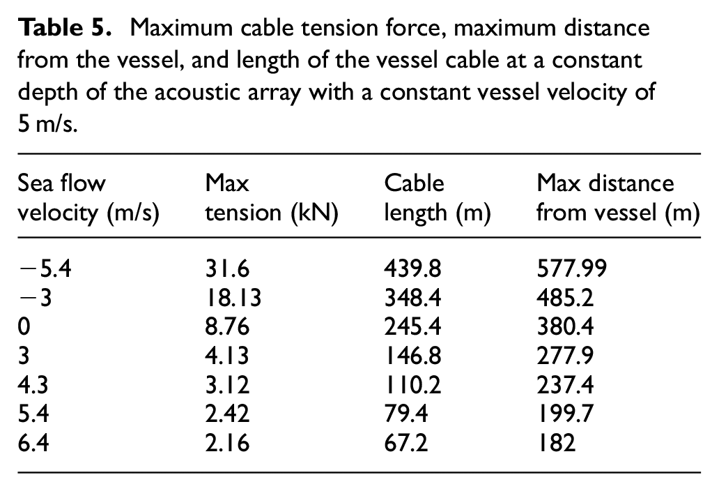
As shown in Figure 9, for high velocities of water flow, the concavity of the cable tension force curve is upwards, and for low velocities of the water flow, the concavity of the cable tension force curve is downwards.

The negative velocities in Table 5 indicate the states in which the velocity of the sea flow and the velocity of the towing vessel are opposite to each other. Here, the relative velocity of the cable-array relative to water increases, which leads to an increase in tension force, a decrease in the angle of the vessel cable relative to the horizon, and an increase in the distance of the acoustic array from the vessel.

Case 3: Three-dimensional mode for varying vessel and seawater movement directions

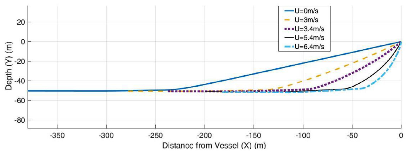
Due to the relative direction of the movement of the vessel and the seawater, it is assumed that the direction of the movement of the seawater is always in the x-direction, and the vessel can have a different orientation. In this case, the velocities of the vessels in the x and z directions are adjusted so that the result is the same as 5 m/s. In these diagrams, U represents the velocity of water flow in the x and Vx, and Vz are vessel velocities in the x and z directions, respectively. Figure 10 shows the geometric shape of the cable-array based on no wind conditions and different vessel orientations. The tension force of the cable is also shown in Figure 11. The maximum tension force of the cable, the maximum distance from the vessel, and the length of the towing cable in the condition of the constant depth of the acoustic array are presented in Table 6.

Figure 10.

Diagram of cable-array in the direction of depth and sea level according to different seawater velocities and angular vessel motion relative to seawater for constant depth of cable-array with vessel velocity of 5 m/s.

Figure 11.

Tension force along with the cable-array in terms of different seawater flow velocities and a constant vessel velocity of 5 m/s for the constant depth of the array and the angular motion of the vessel relative to the seawater.

Table 6.

Maximum tension force of the cable, maximum distance from the vessel, and length of the towing cable at a condition of the constant depth of the acoustic array for a constant velocity of 5 m/s and the angular motion of the vessel relative to the seawater.

Vessel velocity in X direction (m/s)	Vessel velocity in Z direction (m/s)	Sea flow velocity (m/s)	Max tension (kN)	Cable length (m)	Max distance from vessel in X direction (m)	Max distance from vessel in Z direction (m)
5	0	0	8.76	245.4	380.4	0
3.54	3.54	3	5.53	190.6	143.2	289.2
3.54	3.54	−3	15.65	327.2	384.6	254.2
3.54	3.54	0	8.76	245.4	269	269

As shown in all the studied cases, the maximum tension force of the cable-array and the maximum length obtained for the cable-array are related to the situation in which the x component of the vessel velocity is out of direction with the sea flow. It is also found that if the velocity of seawater flow is zero, changing the angle of motion of the vessel (effect of the third dimension) has little effect on the tension force of the cable-array and the length of the vessel cable-array of the cable-array in the steady-state. As a result, it is found that with the angularity of the vessel motion and the non-directionality of its x component velocity with the water flow velocity lead to the maximum length for the vessel cable-array. The minimum length of the cable-array is related to the case where the x component of the vessel motion is in the same direction as the water flow.

Dynamic behavior

For dynamic analysis of cable-array, the boundary condition of velocity and position of the node connected to the vessel at any particular time is considered as the problem’s input based on the operating conditions.

Case 1: Vessel acceleration

At the point of movement initiation (t  =  0 s), the initial position and velocity of the node are both zero, as established by the static analysis. The position and velocity of this node in terms of time are as follows:

$$\mathrm{Velocity}=\left[\begin{array}{ccc}{V}_x+a_{x}t\hfill & 0\hfill & V_z+a_{z}t\hfill \end{array}\right]$$

(9)

$$\mathrm{Position}=\left[\begin{array}{ccc}{V}_{x}t+0.5a_x{t}^2\hfill & 0\hfill & V_{z}t+0.5a_z{t}^2\hfill \end{array}\right]$$

(10)

Table 7 lists the assumptions for this portion of the simulation. Figure 12 depicts the geometry of a cable-array in the water as it accelerates in two separate directions and at different times. This figure illustrates that as time passes from the start of acceleration, the cable tends to become flattered and lose its curvature.

Table 7.

Conditions and assumptions for vessel acceleration simulation.

Parameter	Value
The velocity of the towing vessel	$V=\left[\begin{array}{ccc}3.5\frac{m}{s}\hfill & 0\hfill & 3.5\frac{m}{s}\hfill \end{array}\right]$
Frees surface velocity of seawater	3 m/s
Constant length of towing cable	200 m
Depth of the sea	100 m
Acceleration at t  =  0 s	$a=\left[\begin{array}{ccc}0.2\frac{m}{s^2}\hfill & 0\hfill & -0.2\frac{m}{s^2}\hfill \end{array}\right]$
Duration of the simulation’s runtime	10 s

Figure 12.

Cable-array diagram in the direction of depth and sea level throughout dynamic simulation of vessel acceleration.

In Figure 13, the tension force applied to the cable at different times from the start of acceleration along the cable is depicted, demonstrating that as the vessel accelerates, the tension force along the cable decreases, and as the times from the beginning of acceleration increase, this force also decreases. This research followed about 109 s for a 0.5 ms time step and 619 s for a 0.1 ms time step when the simulation program was run. However, the outcomes of both simulations are relatively comparable. Therefore, the next dynamic simulations have a time step of 0.5 ms.

Figure 13.

Tension force along the cable-array for different time from the start of acceleration.

Case 2: Vessel rotation (U turn)

At the point of movement initiation (t = 0 s), the initial position and velocity of the node are both zero, as established by the static analysis. The position and velocity of this node in terms of time are as follows:

$$\mathrm{Velocity}=\left[\begin{array}{ccc}{V}_x\mathrm{Cos}\left(\frac{V_x}{R}t\right)\hfill & 0\hfill & V_x\mathrm{Sin}\left(\frac{V_x}{R}t\right)\hfill \end{array}\right]$$

(11)

$$\mathrm{Position}=\left[\begin{array}{ccc}\mathrm{RSin}\left(\frac{V_x}{R}t\right)\hfill & 0\hfill & R(1-\mathrm{Cos}\left(\frac{V_x}{R}t\right))\hfill \end{array}\right]$$

(12)

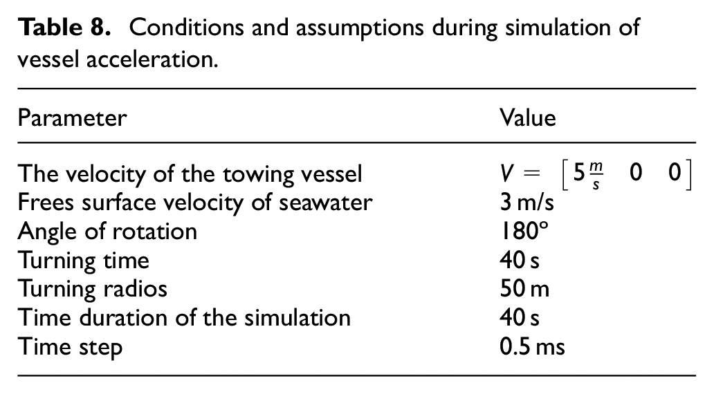
Table 8 provides the requirements and assumptions for the U-turn simulation. Figure 14 depicts the shape of a cable-array in water as it turns in two distinct directions and at various periods. In accordance with this figure, the cable tends to bend into a U-shape as the turning period increases.

Table 8.

Conditions and assumptions during simulation of vessel acceleration.

Parameter	Value
The velocity of the towing vessel	$V=\left[\begin{array}{ccc}5\frac{m}{s}\hfill & 0\hfill & 0\hfill \end{array}\right]$
Frees surface velocity of seawater	3 m/s
Angle of rotation	180º
Turning time	40 s
Turning radios	50 m
Time duration of the simulation	40 s
Time step	0.5 ms

Figure 14.

Acoustic array diagram in the direction of depth and sea level at various times during dynamic simulation for U-turn.

Figure 15 depicts the tension force applied to the cable at various times from the start of cable rotation. It is evident from this figure that when the vessel rotates, the tension force along the cable rises dramatically, and that the force increases again while the vessel’s rotation continues.

Figure 15.

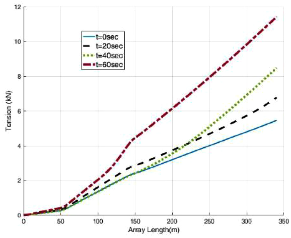
Tension force along with the cable-array for the different times from the start of turning.

Case 3: Cable tightening

Collecting the sonar array from the water is an important operating mode that has a considerable influence on the tension force of the towing cable. In this regard, the speed and acceleration of array cable tightening are a significant challenge. To simulate this, it is assumed that the tangential velocity of the towing cable begins at zero and increases with a constant acceleration to the user-defined maximum value. The cable is then tightened at a constant speed, and the part that is out of the water (the size of its y component is greater than zero) is deducted from the length of the towing cable. Due to the substantial increase in cable tension force, the simulation assumes a restriction for this force while stacking up the sonar array; if the cable tension force exceeds that value (T_max), the cable tightening speed U_t will be calculated using the following equation for the moment equivalent to the counter k:

$$U_t\left(k\right)=U_t(k-1)-\frac{T_{\mathrm{towing}\mathrm{cable}}\left(k\right)-T_{\max }}{1000}\times \mathrm{Dt}\times 0.001$$

(13)

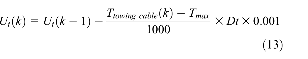
Figure 16 illustrates the Tension force of the towing cable during the stacking of the sonar array for two maximum tension restrictions (9 and 10 kN) with an acceleration of 0.1 m/s² and a maximum speed of 0.5 m/s. In this simulation, the towing vessel’s speed is 5 m/s, and the sea conditions are assumed to be static. According to these diagrams, the tension force develops during the acceleration of the cable stacking up the process and then decreases as the length of the towing cable reduces. The array’s length at the start of the simulation was 340.2 m. After 20 s, the distance reached 331 m for a T_max of 10 kN but 332 m for a T_max of 9 kN.

Figure 16.

Changes in tension force (a) and speed of cable tightening (b) of the towing cable during sonar cable tightening for two maximum tension restriction.

Conclusion

In this study, a cable-array’s static and dynamic behavior under various operating conditions is analyzed using the continuous cable method, and the centralized mass method to solve nonlinear algebraic equations. Static mode operating conditions include a two-dimensional mode for the constant length of the vessel, a two-dimensional mode for the hydrophones’ constant depth, and a three-dimensional mode for variable motion directions of the vessel and seawater. The operating conditions of dynamic mode include vessel acceleration, vessel rotation (U-turn), vessel motion in a choppy sea, and cable stacking. By considering specific drag coefficients in normal and tangential directions, fixed depth of sonar array and linear relationship between sea velocity and depth, the main results are listed as follows:

• The continuous cable method is suitable for two-dimensional mode and has a faster solution procedure compared with the lumped mass method, but it has a singular point in three-dimensional mode. The most important challenge created in the lumped mass method is the long duration of the simulation. To avoid the divergence, the time steps should be selected very small.

• Changing the angle of motion of the towing vessel (impact of the third dimension) has no influence on the tension force of the cable and the length of the vessel cable of the cable-array in the steady-state if the seawater flow velocity is zero.

• Moreover, assuming the constant depth of the cable-array and the constant length of the vessel cable, the maximum cable tension force rises by about 35 and 13 times, respectively, for every 5-fold increase in vessel velocity.

• Assuming a constant depth of cable-array, the cable length increases by five times when the vessel’s speed grows by five times.

• Assuming that the length of the towing cable remains constant, the depth of the array decreases with increasing towing velocity, maximum cable tension force, and array distance from the vessel.

• As time passes since the beginning of acceleration, the cable tends to become flattered and lose its curvature. With vessel acceleration, the tension force along the cable lowers, and with increasing times since acceleration began, this force also decreases.

• As time passes from the start of Turning, the cable tends to form a U shape. With a U-turn of the vessel, the tension force along the cable grows dramatically and also increases with increasing time from the beginning of the turn.

• As time passes from the start of acceleration, the tension force decreases, and the length of the cable-array rises.