Research on surface defect identification of steel balls based on improved K-CV parameter optimization support vector machine

Abstract

Surface defects generated during the production process of steel balls can lead to bearing failures, which makes it crucial to promptly detect and classify these defects. Defects classify is helpful for analysis and improving the production process. An algorithm that incorporates K-fold cross-validation (K-CV) with improved grid search is proposed to optimize the parameters of SVM, in order to detect surface defects with steel balls. Principal Component Analysis (PCA) was employed to reduce the dimensionality of the effective features data. The K-CV algorithm was employed in conjunction with an improved grid search method to find the optimal parameters “c” and “g.” This approach not only reduced the search time but also diminished the influence of individual samples on the model, thereby enhancing its robustness and ultimately improving the classification accuracy. The model’s performance was evaluated using a confusion matrix, and a comparison was made with three other machine learning models. The experimental results demonstrated the effectiveness of the proposed algorithm in classifying defects on highly reflective metal surfaces such as steel balls. The model achieved a classification accuracy of 97.15%.

Introduction

As an important part of bearings, the surface quality of steel balls affects precision, using time and performance of bearings. However, the surface of the steel ball will have flaws such as dents, pits, rust, wear, and hole injuries because of process precision and using wear. These flaws have a crucial impact on bearing accuracy, runnability, and service life.^1,2 Therefore, it is absolutely essential to identify the flaws on steel balls surface before steel balls are accepting, for it can help analyze the reason and improve pass rates. Up to date, the surface quality inspection of ball bearings is usually performed by human operators which easily lead to visual fatigue for workers as well as low detection accuracy. However, defect image is identified and classified through digital signal processing and other technologies, which improve recycling rate of steel balls, and various production accidents caused by unqualified steel ball quality are avoided.

In this context, many researchers have put forward various artificial intelligence algorithms to detect all kinds of surface damage, such as K-nearest neighbor (KNN), ³ artificial neural networks (ANN), ⁴ SVM, ⁵ and Self-Organizing Maps (SOM).^6,7 Many researchers have proposed models for metal surface defect detection. Liu et al. ⁸ employed SOM as a classifier and achieved a classification accuracy of 87%. Yi et al. ⁹ used a CNN to achieve a classification accuracy of 99.05%. Ashour et al. proposed a DST-GLCM-PCA-SVM model for defect detection which combines discrete shearlet transform and gray-level co-occurrence matrix (GLCM) for feature extraction. The final SVM classifier that demonstrated a classification accuracy is 94.1%. ¹⁰

On the other hand, these algorithms are actually subject to certain limitations, such as SVM parameters restricts the accuracy of identification. How to improve the high-efficiency parameter optimization model to improve the practicality of the defect identification algorithm is a problem we need to solve. An algorithm that incorporates cross-validation with improved grid search is proposed to optimize the parameters of SVM.^11,12 Firstly, a larger range is decided which we decide a smaller optimal parameter interval with a larger step. Secondly, a precise search is developed within this optimal interval. This search method enhances the practicality of defect recognition compared to conventional grid method. Before the flaws identification model of SVM, the Principal Component Analysis dimensionality reduction processing of the defect features is carried out, which greatly improves the recognition efficiency and makes the steel ball defect recognition algorithm better meet the real-time requirements. Meanwhile, a solution has been found to address the issue of low performance in conventional SVM identification model, resulting in an enhanced precision for detecting flaws.

An ideal defect image is obtained after preprocessing the steel ball image in a novel approach consists of a dome diffuse LED light source in this paper. The extracted features for classification recognition include grayscale statistical features, geometric features, and texture features of the defect regions. By comparing and analyzing the geometric shape characteristics of the five types of defects, the classification can be performed. What’s more, once we have selected the effective features, principal component analysis is applied to reduce the dimensionality of the feature data. Subsequently, we utilize an improved SVM model to train the defect samples. The validation results of proposed model are then compared and analyzed against those of traditional neural network and conventional SVM models.

Dataset collection

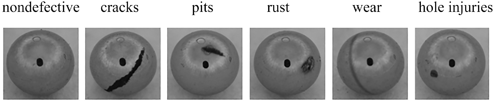
In this work, we trained and tested our classification model with the specific dataset of tiny steel balls defect images, which collected from industrial sites. The surface defects of steel balls are different from steel strips for their own process. The diameter of steel balls is less than 3 mm so that they are more difficult to acquire as well as to find a public dataset about surface defects of steel balls. Our dataset contains five different classes of typical surface defects which are: dents, pits, rust, wear, and hole injuries. Figure 1 shows the experimental setup for capturing images with a diffused dome light source. Figure 2 shows images of five classes of typical surface defects. It’s necessary to note that the black circular reflection in the center of the steel ball image represents the image reflected by the camera lens.

Figure 1.

The experimental setup within a dome diffuse light.

Figure 2.

Five kinds of flaws images by diffuse light.

Methodology

The dimensions of each feature input to the classifier may vary. Without preprocessing, characteristics with larger dimensions can have a significant impact on the classification results, while characteristics with smaller magnitudes may be weakened or even ignored in their influence on the classification results. ¹³ Feature selection is primarily classified into four categories: dimensionality reduction methods, spatial partitioning methods, feature selection methods, and decision tree methods. ¹⁴ By considering intuitive, geometric, grayscale statistical, and transform domain characteristics, a comprehensive characterization of surface defects on steel balls can be achieved, facilitating their analysis, classification, and assessment. ¹⁵ This paper attempts to extract grayscale characteristics, geometric traits, and texture characteristics from images of steel ball defects as description of surface flaws.

The characteristics of steel ball defect images can be summarized from Figure 2. Dents are structural defect that is clearly visible and appears in a crescent shape with low grayscale. Pits have similar characteristics to dents, with clear edges and low grayscale. Rust appears as a texture defect with lower grayscale values, forming in different areas. Hole injuries are approximately circular with clear edges and lower grayscale values. Wear are texture defects that are difficult to judge based solely on shape and grayscale.

Flaws characteristics extraction of surface defects and data preprocessing

After discussing shape characteristics, discriminative geometric characteristics were employed, including rectangular factor, length-to-width ratio, ovalness, and degree of irregularity. It is a statistical geometric feature that measures the degree of resemblance between an object or region and a rectangle which is called rectangular factor. It is computed by calculating the ratio of the object or region’s perimeter to the perimeter of its minimum bounding rectangle. It can be very useful on dents. Eccentricity is another statistical geometric feature that describes the elongation or roundness of an object or region. It quantifies how much an object deviates from a perfect circle. Degree of irregularity can be calculated using various methods, but a commonly used approach is based on the perimeter and area of the shape. Hu Moments refer to a collection of mathematical descriptors or moments utilized for characterizing an object’s shape in the fields of image analysis and pattern recognition. ¹⁶ The role of normalized central moments is to provide a standardized measure of an object’s shape or distribution of intensity values in an image, independent of factors like translation, scale, and rotation. Variation caused by these factors can be eliminated by normalizing the central moments, making the moments more robust and suitable for comparison and recognition tasks.

Wear defects are indeed different from other kinds of flaws. While other flaws may be caused by factors like impact, corrosion, or manufacturing errors, wear defects specifically result from the gradual removal or deterioration of material due to friction, rubbing, or abrasive contact. The surface appearance is even as well as the spatial distribution is regular. Texture statistical methods quantify and analyze the patterns, variations, and spatial relationships within an image or surface to describe its texture characteristics. ¹⁷ Texture characteristics of an image can be described by its grayscale distribution characteristics, statistical features obtained from computing the GLCM between pixel pairs, as well as global and local binary patterns (LBP). These descriptive methods provide texture feature information from different levels and perspectives. Depending on the specific problem, suitable methods can be chosen to describe and analyze texture characteristics.

PCA is a method to get the principal components of the original data by calculating the covariance matrix or correlation matrix. This method works by transforming the original variables of the data into a new set of uncorrelated variables, which means, high-dimensional data can be reduced to K dimensions by selecting the top K principal components, so as to achieving dimensionality reduction.^18,19

First, the data has to be preprocessed in order to remove noisy points. Then we have to calculate the covariance matrix of the preprocessed data. Assuming the preprocessed sample dataset is available that is denoted as X. The dataset X consists of N data points, where each data point has d-dimensional features. The sample matrix N could be as N $\in {\mathrm{R}}^{m\times n}$ . In this context, the rows correspond to samples while the columns represent dimensions. The mean vector of m samples is given by

$$\overline{\mathrm{X}}=\frac{1}{m}\sum _{i=1}^m{x}_i$$

(1)

where $\mathrm{x}\in \mathrm{X}$ , $\mathrm{X}=\{{\mathrm{x}}_1,\dots ,{\mathrm{x}}_{\mathrm{m}}\}$ , ${\mathrm{X}}_{\mathrm{i}}=\{{\mathrm{x}}_{\mathrm{i}1},\dots ,{\mathrm{x}}_{\mathrm{in}}\}\in {\mathrm{N}}^{\mathrm{n}}$ , i = 1, …, m.

The covariance matrix K could be given by

$$\mathrm{K}=\frac{1}{m}\sum _{i=1}^m{x}_i^T{\overline{x}}_i=\frac{1}{m}\overline{X}{\overline{X}}^{\mathrm{T}}$$

(2)

where $\overline{\mathrm{X}}$ represents matrix of $\overline{\mathrm{x}}$ , which is $\overline{\mathrm{X}}$ = ( $\overline{\mathrm{x}}$ ₁, …, $\overline{\mathrm{x}}$ _i) $\in {\mathrm{N}}^{m\times n}$ .

Secondly, compute eigenvectors and eigenvalues. Eigen is decomposed with covariance matrix to obtain eigenvectors and their corresponding eigenvalues. Therefore, the eigenvalue matrix Λ was obtained as well as the eigenvector matrix. The eigenvector matrix is then orthogonalized to form matrix P.

$${\mathrm{P}}^{\mathrm{T}}\mathrm{KP}=\Lambda$$

(3)

where $\Lambda =\mathrm{diag}({\lambda }_1,{\lambda }_2,\dots ,{\lambda }_{\mathrm{m}})$ , $P{P}^T=1$ .

Finally, the data is transformed. By multiplying the original sample data with the dimensionality reduction matrix, the new sample data after dimensionality reduction is obtained. In other words, the data sample matrix is transformed from the original high-dimensional space to a new low-dimensional space.

Main principle of SVM algorithm

SVM that is a machine learning algorithm commonly is used on classification and recognition works. The fundamental idea behind SVM is to identify an optimal hyperplane in a high-dimensional space that effectively segment data points into distinct categories.^20,21 Therefore, SVM aims to optimize the margin, which is defined as the closest proximity between the hyperplane and the nearest sample sets belonging to different categories.^22,23 The learning strategy of SVM is to maximize the interval, which can be formalized as a problem of solving convex quadratic programing, which is also equivalent to the problem of minimizing the regularized hinge loss function. The learning algorithm of SVM is the optimization algorithm for solving convex quadratic programing.

The identification on surface flaws with steel balls presents a typical example of non-linear discrimination task. Employing a SVM classifier offers a potential approach for effectively classifying these defects. The algorithm follows the following steps:

The problem of solving the maximum segmentation hyperplane of the SVM model can be expressed as the following constrained optimization problem, which can be solved using the Lagrange method. Denote K (x_i, y_i) as the kernel function as well as C as a penalty parameter. In order to meet the classification requirements of the kernel space, the Gaussian radial basis function is selected as the kernel function which has a wide applicability. It is suitable for various data sizes. It is given by

$$\mathrm{K}({\mathrm{x}}_{\mathrm{i}}·\mathrm{x})=\exp \left(\frac{-\parallel {\mathrm{x}}_{\mathrm{i}}-{\mathrm{x}}_{\mathrm{j}}{\parallel }^2}{{\sigma }^2}\right)$$

(4)

where x_i and x_j are the feature vectors of the training samples, and $\sigma$ is a parameter that controls the width of the Gaussian distribution.

The goal of the optimization problem is to find an optimal set of weight vector w and intercept b that maximizes the separation between the classification boundary and the support vectors and minimizes the misclassification error.

$$min\mathrm{L}(\mathrm{w},\mathrm{b},\alpha )=\underset{\alpha }{min}\frac{1}{2}\sum _{\mathrm{i}=1}^{\mathrm{i}}\sum _{\mathrm{j}=1}^{\mathrm{i}}{\mathrm{y}}_{\mathrm{i}}{\mathrm{y}}_{\mathrm{j}}{\alpha }_{\mathrm{i}}{\alpha }_{\mathrm{j}}\mathrm{K}({\mathrm{x}}_{\mathrm{i}},{\mathrm{x}}_{\mathrm{j}})-\sum _{\mathrm{j}=1}^{\mathrm{i}}{\alpha }_{\mathrm{j}}$$

(5)

where s.t. $\sum _{i=1}^i{y}_i{\alpha }_i=0,0\le {\alpha }_i\le C,i=1,2,\cdots ,m$ . The input training dataset are {(x₁, y₁), (x₂, y₂), ···, (x_m, y_m)}, x_i∈R_n, y_i∈ {− 1, 1 } , i  = 1, 2, ···, m.

Use the obtained weight vector w and intercept b to construct a decision function which is given by

$$\mathrm{F}\left(\mathrm{x}\right)=\mathrm{sgn}\{({\mathrm{w}}^{*}·\mathrm{x})+{\mathrm{b}}^{*}\}$$

(6)

When classify the flaws on steel balls with SVM algorithm, it is necessary to adjust the parameters of the kernel function and penalty parameter to improve the recognition accuracy. Instead of randomly selecting parameters, the K-CV optimization algorithm is adopted for the optimal parameters so as to get a more precise SVM model.

Optimization of SVM parameter model with K-fold cross validation algorithm

The principle of the K-CV algorithm is as follows: The original data is divided into K sets. For each subset, there is a validation set, and the remaining K−1 subsets are used as the training set, resulting in K models. The average accuracy of a classifier can often be assessed by measuring its performance on the validation set of the K-model. In traditional grid search methods, the grids are evenly divided, resulting in a large computational load. An improved grid search method is proposed by this paper to optimize the parameters of SVM. Figure 3 shows the improved the parameter optimization of SVM model algorithm process.

Figure 3.

Main flowchart of the SVM parameter optimization algorithm.

Initially, a coarse search with a large step size and a wide range is performed to determine the optimal parameter range for the coefficient of penalty and the kernel parameter. ¹¹ Within the identified optimal range, a fine search is conducted with a smaller step size to refine the search. Finally, the optimal parameters are obtained. The main process of the algorithm is as follows:

• (1) Preprocess the collected images. A total of 214 images of five types of steel ball defects are collected, and the effective feature vectors are extracted for each sample. The collected feature data is divided into training data and prediction data, and the training data is labeled with their corresponding types.

• (2) Apply the PCA algorithm to reduce the dimensionality of the training data and extract the feature vectors of the defect images after dimensionality reduction.

• (3) Determine the optimal number of clusters, K, and then use the K-CV algorithm and an improved grid search method to find the optimal solution for the SVM parameters.

• (4) Use the feature vectors obtained in step (2) and the optimal solution for the parameters obtained in step (3) as inputs to train the SVM classifier.

• (5) Apply the PCA algorithm to the training samples of the defect images to reduce dimensionality, extract the feature vectors, and then input them into the SVM model for prediction.

• (6) Compare the predicted labels from the model with the actual labels of the prediction data to obtain the accuracy of predicting steel ball defects.

Experiment and analysis

Feature selection experiments

An effectiveness verification experiment for geometric feature extraction was conducted using 214 samples and five types of defect data. An example of sample images is shown in Figure 4. Geometric features including rectangular factor, length-to-width ratio, ovalness, degree of irregularity, and seven unaltered measures, for a total of 11-dimensional data, were extracted. The classifier used in the experiment was the classical KNN algorithm. The training dataset consisted of 120 samples with five types of defects, and the test dataset included 75 samples, with each type of defect being evenly distributed in the dataset. Table 1 shows the recognition rate with all kinds of flaws. The experimental results indicate that geometric characteristics are highly successful in classifying various types of defects except for rust, with a classification accuracy reaching up to 85%. However, when considering the detection of rust defects, the overall accuracy drops to only 73.3%.

Figure 4.

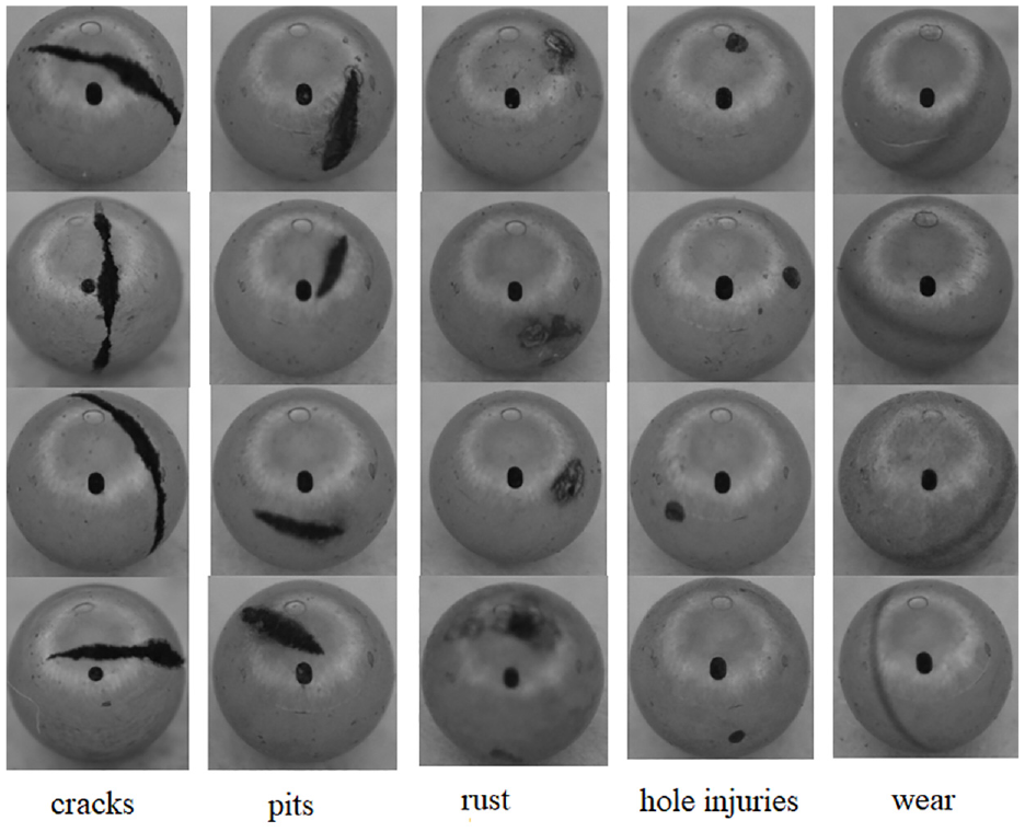
Five kinds of defects of steel balls images.

Table 1.

Five types of defects identification results of geometric characteristics with KNN.

Sample	Hole injuries	Pits	Dents	Rust	Wear	Recognition rate (%)	Total recognition rate (%)
Hole injuries	14	0	0	1	0	93.3	73.3
Pits	1	13	0	1	0	86.7
Dents	0	2	12	0	1	80
Rust	0	2	0	12	1	80
Wear	0	2	7	1	5	33.3

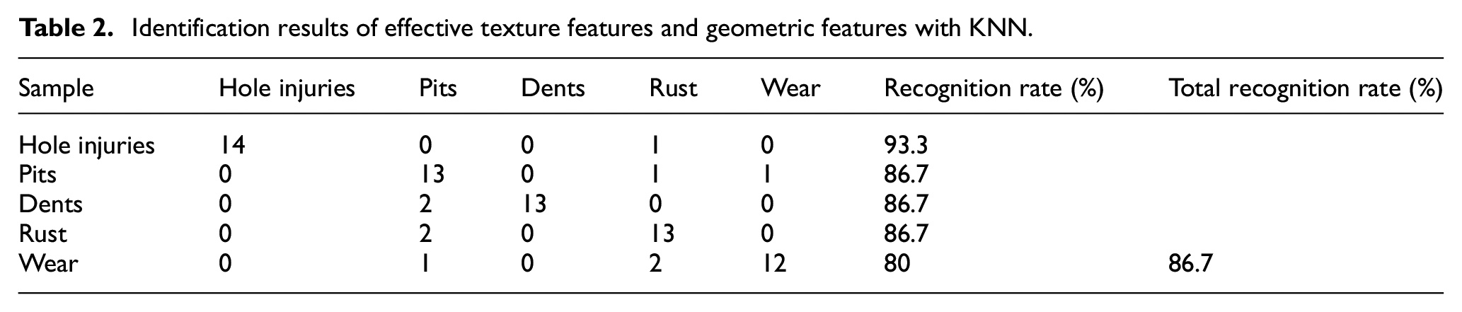
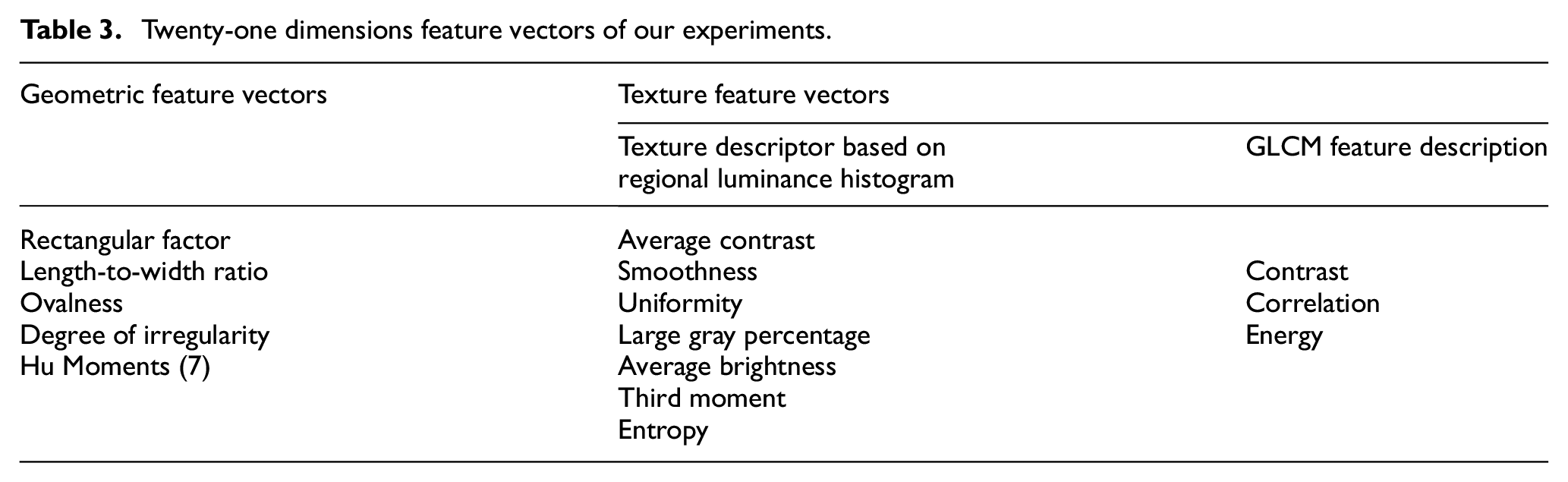
For texture-based defects such as rust or wear, the fusion of texture features and geometric features is adopted. The fused feature vector is then used for classification and recognition. Here, we added 11-dimensional texture features, including average contrast, smoothness, uniformity, large gray percentage, average brightness, third moment, entropy, contrast, correlation, and energy. The wear defect from Table 2 is classified for its recognition rate reach to 80% compare to Table 1. The overall recognition rate has been increased from 30% to 70%. It proves that these texture features are very useful to recognize texture-based flaws besides geometric feature flaws. It also addresses the issue of classifying texture-related defects such as wear and rust, which cannot be effectively classified using solely geometric features. The total recognition rate is up to 86.7%. The training dataset includes instances where the surface of the same steel ball exhibits both texture defects and long pit defects, and the proposed model is able to accurately identify and classify them. It can be concluded that a 21-dimensional feature vector is effective for classifier recognition, which is shown in Table 3. Finally, 21-dimensional feature vectors are reduced to 10 dimensions by performing principal component analysis dimensionality reduction. This reduction reduces the computational complexity of the data and provides a foundation for training the SVM model.

Table 2.

Identification results of effective texture features and geometric features with KNN.

Sample	Hole injuries	Pits	Dents	Rust	Wear	Recognition rate (%)	Total recognition rate (%)
Hole injuries	14	0	0	1	0	93.3	86.7
Pits	0	13	0	1	1	86.7
Dents	0	2	13	0	0	86.7
Rust	0	2	0	13	0	86.7
Wear	0	1	0	2	12	80

Table 3.

Twenty-one dimensions feature vectors of our experiments.

Geometric feature vectors	Texture feature vectors
	Texture descriptor based on regional luminance histogram	GLCM feature description
Rectangular factor	Average contrast
Length-to-width ratio	Smoothness	Contrast
Ovalness	Uniformity	Correlation
Degree of irregularity	Large gray percentage	Energy
Hu Moments (7)	Average brightness
	Third moment
	Entropy

Improved grid search algorithm result analysis

To validate the PCA and SVM defect algorithm based on K-CV optimization, it is recommended to use the MATLAB software for simulation testing. The LIBSVM library developed by Chang and Lin ²⁴ provides built-in training and prediction functions that can be used to implement the SVM algorithm. The C-SVC type is used for training SVM model. The training dataset consists of 144 sample data points, with an equal proportion of five types of defects. Additionally, the testing dataset consists of 70 randomly sampled data points. The RBF kernel was used. After performing PCA on the 21-dimensional feature vector, the data dimension was reduced to 10 dimensions, retaining 99% of the variance.

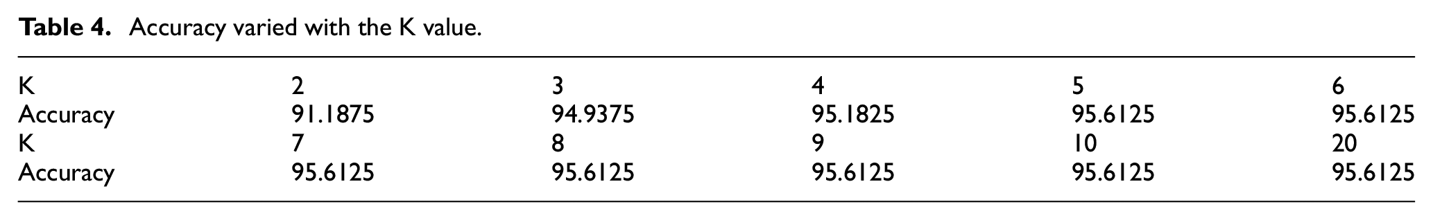
Determining the optimal number of clusters, K. Firstly, the training sample images are read, and the PCA algorithm is applied to reduce the dimensionality of the training samples and extract the feature vectors of the defect images. Combined with the K-CV algorithm, the SVM model parameters are optimized, and the variation of defect recognition accuracy with K value is shown in Table 4. From Table 4, it can be observed that when K ≥ 5, the defect recognition accuracy reaches its maximum value of 94.6125%. To reduce computational complexity, we choose K as 5.

Table 4.

Accuracy varied with the K value.

K	2	3	4	5	6
Accuracy	91.1875	94.9375	95.1825	95.6125	95.6125
K	7	8	9	10	20
Accuracy	95.6125	95.6125	95.6125	95.6125	95.6125

We use the K-CV algorithm and the improved grid search method to determine the optimal SVM parameters. Figure 5 shows the contour plot obtained using a coarse search with large steps, where the x-axis and y-axis represent the logarithmic values with base 2 of the parameter c and g, respectively. The contour lines represent the defect recognition accuracy obtained by the K-CV algorithm for the corresponding values of c and g. Figure 6 shows a 3D view obtained using a coarse search with large steps, where the ranges of both c and g are set to [2⁻²⁰, 2²⁰] with a step size of 0.9. The optimal penalty coefficient c is found to be 10.5561, the kernel function parameter g is 0.87055, and the best CV accuracy is 91.9167%. From Figure 6, it can be observed that the range of c can be narrowed down to [2⁻⁵, 2⁵], and the range of g can be narrowed down to [2⁻⁵, 2⁵] with a step size of 0.2. Based on the coarse selection above, we can further utilize the SVM training function for fine parameter selection to reduce unnecessary calculations and save time. Conversely, if a fine-grained search is applied from the beginning, it will consume a lot of time. The contour plot after fine-grained parameter selection is shown in Figure 7, and its 3D view is shown in Figure 8. From Figures 7 and 8, it can be seen that after fine-grained parameter selection, the optimal penalty coefficient c is 5.6569, the kernel function parameter g is 1.4142, and the best CV accuracy is 95.8333%.

Figure 5.

Big step parameter selection in contour map.

Figure 6.

Big step parameter selection in 3D view..

Figure 7.

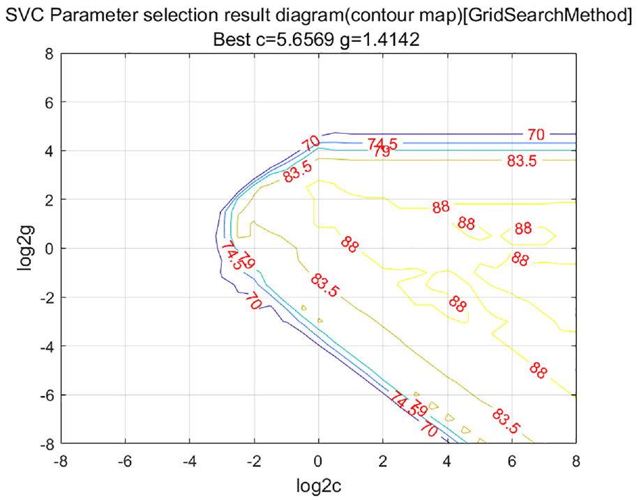
Small step parameter selection in contour map.

Figure 8.

Small step parameter selection in 3D view.

Under the condition of the optimal number of clusters K as 5, the range of c is set to [2⁻³, 2⁵], and the range of g is set to [2⁻⁸, 2⁸], with a step size of 0.5. Five experiments are conducted for both the traditional grid algorithm and the improved grid algorithm to determine the average optimization time, as shown in Table 5. From Table 5, it can be seen that under the same recognition accuracy, the improved grid search algorithm is significantly better than the traditional grid search algorithm.

Table 5.

Comparison of optimization time with traditional algorithm.

Algorithm	The traditional grid search method	Improved grid search method
Time (s)	168.73	18.7

Model prediction and result analysis

The SVM model was trained with the optimal parameters c and g obtained above on 144 training samples. Then, we used this trained model to predict the classification of 70 test defect samples. Figure 9 reports the prediction results obtained using the K-CV algorithm and the improved grid search algorithm. Through Figure 9, we can see that the model was able to correctly classify 68, while it misclassified two images that came as follows: one images of class rust and one images of class wear. As a result, the proposed model achieved an accuracy of 97.15%.

Figure 9.

Classification result of actual and expected test data.

A confusion matrix was usually used to evaluate the performance of classifier model.^25,26 It is a table containing information about the actual ratings (classified by humans) and the predictive ratings that the classifier predicts. The columns are the actual class while the rows are the predicted class, and the performance of the classifier is usually evaluated using the data contained in the matrix.^7,27 The confusion matrix of the proposed model K-CV SVM is as Table 6. In order to evaluate the performance of the classifier, four metrics of accuracy, precision, recall, and F1 score is calculated. Accuracy represents the ratio of correctly identified by the classifier. Precision represents the classifier’s success rate of classifying the correct cases for each group of the classified classes. Recall represents the classifier’s success rate of not classifying wrong cases to another class (or group) of the classified classes. F1 score represents the harmonic average of the precision and recall. All the metrics are calculated as:

$$\mathrm{Accuracy}=\frac{\mathrm{TP}+\mathrm{TN}}{\mathrm{TP}+\mathrm{FP}+\mathrm{TN}+\mathrm{FN}}$$

(7)

$$\mathrm{Precision}=\frac{\mathrm{TP}}{\mathrm{TP}+\mathrm{FP}}$$

(8)

$$\mathrm{Recall}=\frac{\mathrm{TP}}{\mathrm{TP}+\mathrm{FN}}$$

(9)

$$\mathrm{F}1\mathrm{Score}=2\times \frac{\mathrm{Precision}\times \mathrm{Recall}}{\mathrm{Precision}+\mathrm{Recall}}$$

(10)

Table 6.

The confusion matrix of the proposed model K-CV SVM.

Target class
Output class	Sample	Hole injuries	Pits	Dents	Rust	Wear
	Hole injuries	15	0	0	0	0
	Pits	0	15	0	0	0
	Dents	0	0	13	0	0
	Rust	0	0	0	13	1
	Wear	0	0	1	0	12

Here, TP, TN, FP, FN means true positive, true negative, false positive, and false negative.

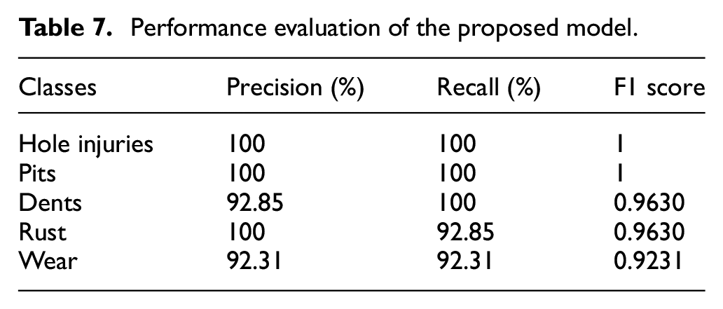
Therefore, the performance evaluation of our proposed model can be calculate in Table 7. We can conclude that the classifier’s performance was excellent. The “precision” ranges between 92.31% and 100%. In steel ball detection, “recall” is the most important metric as it emphasizes not missing any defective steel balls and aims to identify all true positive defects. In this case, minimizing false negatives, or missed detections, is crucial. Therefore, a higher recall value indicates that the system is better at capturing true defects, reducing the likelihood of missing any defective steel balls. On the other hand, a slight increase in false positives is more acceptable since the focus is on not missing any defects. It provided high rates, ranging from 92.31% to 100%. What’s more, “F1 score” reflects the efficiency and effectiveness of the model. It is close to “1,” ranging from 92.31% to 100%. The following conclusions can be drawn: the recognition rate for each type of defect significantly improved, demonstrating that this method is effective and feasible.

Table 7.

Performance evaluation of the proposed model.

Classes	Precision (%)	Recall (%)	F1 score
Hole injuries	100	100	1
Pits	100	100	1
Dents	92.85	100	0.9630
Rust	100	92.85	0.9630
Wear	92.31	92.31	0.9231

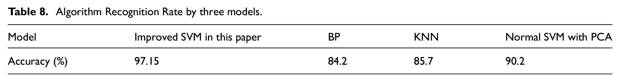
By using the same training and testing data, a three-layer BP neural network was constructed. The Sigmoid transfer function (logsig) was applied in each layer of the BP neural network. The hidden layer was determined to have five neurons. The model training was performed using the variable learning rate method with momentum. When classifying and predicting the 70 samples, it was observed that the BP neural network encountered difficulties distinguishing between rust and cyclic roughness, as well as confusion between long depressions and cracks. The final classification accuracy was 84.2%. Similarly, when using the KNN model with k as 7, the calculated classification accuracy was 85.7%. After applying PCA dimensional reduction, the classical SVM model achieved a classification accuracy of 90.2%. In comparison, the SVM model demonstrated higher classification accuracy. By utilizing the proposed K-CV algorithm and improved grid search method to optimize the SVM parameters, the predictive model achieved an accuracy of 97.15%. Algorithm Recognition Rate by three models is shown by Table 8.

Table 8.

Algorithm Recognition Rate by three models.

Model	Improved SVM in this paper	BP	KNN	Normal SVM with PCA
Accuracy (%)	97.15	84.2	85.7	90.2

Conclusion

A novel SVM parameter optimization algorithm combining cross-validation with an improved grid search is proposed. After effective feature selection for surface defects on steel balls, the normalized raw data is obtained by applying PCA for dimensionality reduction. The algorithm starts with a coarse search using larger step sizes to determine an initial optimal parameter range. Then, a fine-grained search is performed within this range to obtain the optimized SVM parameters “c” and “g.” Based on real measured data from the industrial site, a prediction model is established, which effectively mitigates the impact of large errors from individual samples and performs well in predicting steel ball defects.

The effectiveness of the proposed model is verified through multiple experiments, with the following key findings:

Effective feature selection for steel ball images with both structural and texture defects should include geometric and texture features. A 21-dimensional feature vector is found to be effective in identifying surface defects. Through PCA dimensionality reduction, the effective feature data is simplified to 10 dimensions.

The SVM parameter optimization algorithm combining cross-validation with an improved grid search is proven to be effective. The proposed model is evaluated using accuracy, precision, recall, and F1 score metrics through confusion matrix analysis. A comparison is also made with BP neural network, KNN, and traditional grid search SVM models. The algorithm improves the accuracy of defect recognition on steel ball surfaces and reduces the search time for optimal SVM parameters. It exhibits stable performance in steel ball surface defect detection applications.

In the future, further experiments will focus on replacing SVM with other deep learning algorithms such as GAN, YOLO, and SOM, which is applied in real industrial environments.