Sage Journals: Discover world-class research

Abstract

Numerical simulation is becoming an important research method in the field of supersonic flow. Its accuracy and reliability have always been the key to its further application and the focus of current researches. In this study, a series of numerical simulations of transverse supersonic jet in supersonic free flow are carried out based on Reynolds averaged (RANS) solver. Firstly, the flow field structure obtained by different calculation cases is studied, and the mechanism of the difference of flow field structure is described. Furthermore, by changing the accuracy of difference scheme for the convection term and the turbulence model, the different simulation results are compared with the experimental data. The deviation from numerical simulation compared with the experiment is further analyzed to clarify the critical factors affecting the calculation reliability. The results show that improving the accuracy of the scheme cannot effectively improve the calculation results, while choosing an appropriate turbulence model can be helpful to improve the calculation accuracy. When the numerical simulation of jet flow mixing in supersonic flow field is carried out, the conclusions of this study can provide a support for determining the numerical model method and error analysis.

Keywords

RANS simulation jet in supersonic cross flow calculation accuracy analysis

Introduction

Hypersonic aircraft powered by scramjet can reach all places in the world within 2 h, attracting countries to compete for research and development. The scheme of using wall normal fuel injection in scramjet combustor has become one of the simplest and most effective fuel mixing enhancement methods,¹ which has the characteristics of simple configuration and high mixing efficiency. In its flow field, jet/boundary layer interaction, large-scale shear vortex, shock/wake interference and other issues are hot topics in the study of turbulent flow and mixing mechanism under supersonic conditions.^2–4 At the same time, the abundant experimental data provide a basis for further improvement of the supersonic turbulence model and numerical methods. In recent years, quite a few scholars have carried out a lot of relevant experimental and numerical research work, and Huang⁵ and Choubey et al.⁶ have made comprehensive reviews of this work.

In recent years, visual experimental techniques have been used to observe the transverse jet flow field in supersonic flow,⁷ and some classical understandings and conclusions have been formed on its flow field structure and mixing characteristics. In the early experiments of Ben yakar⁸ and Santiago and Dutton,⁹ the non-reacting transverse jet flow field was observed. The flow field under different operating cases has a common basic structure, as shown in Figure 1. The flow field contains complex three-dimensional shock waves, recirculation zones, large-scale vortex structures in the shear layer and jet wake regions. The barrel shock around the jet shrinks upward to form a Mach disk, and the incoming stream is compressed in front of the jet region to generate a bow shock. The jet injection results in the separation of the upstream boundary layer and induces horseshoe vortices near the wall. The vortex structures in the jet shear layer and wake play a dominant role in the mixing of fuel and air. Gruber et al.¹⁰ found that the most important factor controlling the penetration depth of jet is the momentum ratio of incoming flow and jet. Erdem and Kontis¹¹ noticed in the experiment that the change of jet penetration with respect to the momentum ratio is nonlinear. Portz and Segal¹² studied experimentally the penetration of gas jets in supersonic flow, and revealed that at low Mach numbers around a value of 1.6, the thickness of boundary layer plays an important role in near-field jet penetration, while with the increase of Mach number, the influence of the thickness of boundary layer gradually decreases.

Figure 1.

Schematic diagram of transverse jet in supersonic flow.¹³

In addition, numerical simulations on many different platforms and methods further illustrate the fine structure and mixing mechanism of transverse jet. The near-field mixing process is controlled by the shear vortices induced by K-H instability in the jet shear layer,¹³ whose entrainment and stretching promote the mixing of fuel and air.¹⁴ The far field mixing process is controlled by the counter rotating vortex pair (CVP) and the Ω-shape vortex, and the mass diffusion plays a leading role.¹⁵ The horseshoe vortex is induced by the separation of the upstream boundary layer, which is close to the wall and spreads around the periphery of the jet to the downstream, and hardly participates in the mixing process.¹⁶

Sun and Hu^17,18 used direct numerical simulation to study the detailed structure of the transverse jet, such as the main reverse vortex, the upper tail reverse vortex, and the surface tail reverse vortex pair of the sonic jet in the supersonic transverse flow. The research shows that it is generated by the vortex distortion in the near field shear layer of the evolving jet and the pressure difference between the upwind and leeward of the jet.¹⁹ Watanabe et al.²⁰ described the turbulent structure of vertical jet in supersonic flow through LES research, and revealed that the contour of jet boundary is formed by the large-scale vortex on the windward side of jet plume. In their other work,²¹ it was found that the jet characteristics were strongly affected by the incoming flow conditions, and the time average trajectory of the jet was controlled by the momentum ratio J. In addition, the momentum ratio has little effect on the size and shape of coherent structures in the shear layer, but will increase the convection velocity of these structures. Rana et al.²² realized the generation method of turbulent inlet based on digital filter in the numerical study of transverse jet. They noticed that the K-H instability occurred on the jet shear layer on the windward side of the jet plume, and then developed into large-scale vortices, promoting the mixing of air and fuel. You et al.²³ conducted Detached Eddy Simulation (DES) and RANS simulation respectively for jet flow and mixing in scramjet combustor. The comparison results show that DES method captures the dynamics of turbulent structure well, and provides results of mixing efficiency that are more consistent with experiments than RANS. Although LES provides high resolution and fine structure, RANS is a more efficient numerical tool, which can also reproduce correct flow field structure and predict roughly accurate parameter distribution.

When using RANS for numerical simulation, the grid resolution and numerical scheme adopted in the calculation will have different effects on the shape of shock wave and vortex structure and the jet distribution characteristics in the flow field. Sun and Timin²⁴ used the high-precision WENO scheme, combined with the k–ε two equation turbulence model, to accurately simulate the interference flow field formed by the transverse jet in supersonic flow. Unweighted or weighted essentially non oscillatory schemes (ENO or WENO) can correctly capture shock waves without generating significant numerical oscillations,^25–27 but they are usually too dissipative and have a significant damping effect on turbulence. The applicability of such schemes to turbulence problems can be improved by adding flux stencils based on central difference or reducing high wave number dissipation of specific stencils through limiters.^28,29 Huh and Lee³⁰ compared the performance of RoeM and HLLE flux schemes in the RANS solver, and the results showed that the complex shock structure led to the instability of the numerical solution. The original Roe scheme failed to obtain a stable solution, while the RoeM scheme and HLLE scheme obtained better results.

At the same time, different turbulence models have their own adaptation to the physical situation, and their versatility is poor. Zhang et al.³¹ improved the calculation accuracy of the model for low-speed incoming transverse jet by adding strain rate tensor to the Spalart Allmaras (S-A) turbulence model. Volkov et al.³² compared Spalart-Allmaras, k-ε, k-ω and SST turbulence models in the simulation of transverse jet, it is found that SST model can get the results consistent with the corresponding experimental data in a wide range. Huang et al.³³ has done similar work, and also believes that SST turbulence model has advantages in predicting this type of problem. However, these numerical simulation work did not pay attention to the influence of calculation methods on the accuracy of results. This paper systematically analyzed the calculation results of different precision numerical schemes and different turbulence models, and obtained the corresponding conclusions, hoping to provide a meaningful reference for the numerical simulation of such problems.

Physical model and numerical settings

Based on the jet experiments of Santiago and Dutton,⁹ Everett³⁴ and VanLerberghe,³⁵ this paper verifies the reliability of the numerical method and further analyzes the factors affecting the numerical accuracy. Table 1 shows conditions of supersonic inflow and jet for the case. In the experiment, the stagnation pressure of supersonic free incoming air is 241 kPa, the stagnation temperature is 295 K, the Mach number is 1.6, and the corresponding static pressure is 56.7 kPa, the static temperature is 195.1 K. A circular injection device with a diameter of d = 4 mm is installed on the flat plate. The nitrogen jet is injected into the supersonic free air flow along the vertical direction of the wall. The Mach number of the jet is 1.0, the total temperature and pressure are 295 K and 476 kPa respectively, and the corresponding static temperature and pressure are 245.83 K and 251.46 kPa respectively. The thickness of the boundary layer of the incoming flow is matched with the experiment at x/d = −5, δ = 0.775d=3.1 mm. Reynolds number of incoming flow is ${Re}_{δ} = ρ U δ / μ = 1.1 \times 10^{5}$ where all parameters here are given to their inlet values and the boundary layer thickness δ is the characteristic length, and the momentum flux ratio of jet/incoming flow is 1.7.

Table 1.

Conditions of supersonic inflow and jet.

	Supersonic inflow	Sonic jet
Ma	1.6	1.0
P(kPa)	56.7	251.46
T (K)	195.1	245.83
Re_δ	1.1 × 10⁵
J	1.7
d(mm)	4

The convective terms, that is, inviscid terms, are discretized by the second order AUSM + UP scheme³⁶ or the fourth order central difference/WENO hybrid scheme³⁷ with low dissipation, while the diffusive terms, that is, viscid terms, are discretized by the second order central difference scheme. And the second order TVD-type explicit Runge Kutta method is used for time integration. The k-ω SST³⁸ and k-ω 2006³⁹ turbulence models were used to compare numerical results. The numerical simulation program is our own three-dimensional unsteady GPU solver for solving compressible NS equations. In incompressible flow simulations, the strong coupling of velocity and hydrodynamic pressure necessitates the calculation of the pressure Poisson equation. While in compressible flow simulations here, velocity and pressure are decoupled, and pressure is calculated through the gas state equation. The detailed description of this solver is referred to Lai et al.⁴⁰

The calculation region and boundary condition settings of numerical simulation are shown in Figure 2. The three-dimensional calculation region includes the upstream supersonic turbulent boundary layer zone, central jet injection zone and downstream buffer zone. Based on the boundary layer thickness of 0.775d (3.1 mm) at x/d = − 5, it is calculated through numerical simulation that the supersonic turbulent inlet should be 250 mm before x/d = − 5, so the length of the supersonic boundary layer zone is 62.5d. The coordinate origin is located at the center of the orifice, and the lengths of flow direction, span direction and normal direction are 87.5d × 10 d × 9 d, respectively. The flow direction position of the central focus region is 5d in front of and 5d in the back of the coordinate origin, its normal position is within 3.75d, and its spanwise position is 2d in the left and right of the coordinate origin. A buffer zone with a length of 15d is set at the downstream, and a relatively coarse grid is set along the flow direction in order to prevent the numerical disturbance at the outlet propagating upstream along the boundary layer. The initial conditions for the whole computational domain of all numerical cases are set to the same as the incoming flow state at inlet before the RANS simulations. The RANS simulations for all cases in the present work are steady, and all calculations are converged.

Figure 2.

Calculation domain and boundary condition settings.

Numerical results and discussion

Grid independence verification

The 3.96 million hexahedral grid is used as a benchmark case to refine the grid and investigate the influence of grid density on the numerical results. Three sets of hexahedral structural grids with different grid numbers of 3.96 million, 7.92 million and 11.76 million are used here for calculation. The grid length from the first layer of the wall is set to 0.001 mm. The grid in the direction perpendicular to the wall is stretched according to an exponential function from the wall to 0.3 d, and then the grid is uniformly distributed from 0.3d to 3.75 d. In addition to the local refinement near the jet outlet, the grid in the spanwise and flow direction is equally spaced. The mesh of coarse grid case for streamwise central section of the whole domain is shown in Figure 3(a), and the zoomed mesh for near-wall region near the jet overlaped by the Mach number contour is given in Figure 3(b). And the y⁺ value is calculated to be 1.025, the same for all cases with various meshes, schemes and models.

Figure 3.

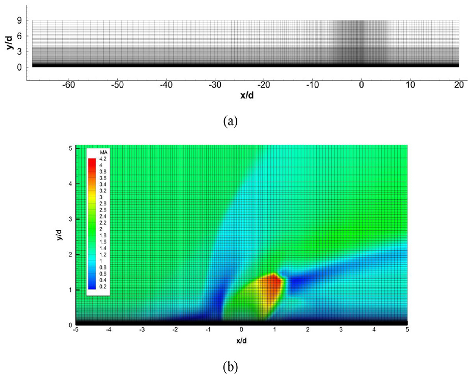
The mesh of coarse grid case for streamwise central section of: (a) the whole domain and (b) the zoomed near-wall region near the jet overlaped by the Mach number contour.

Figure 4 shows the distribution comparison of streamwise and transverse velocities of three sets of computational grids on the four sections x/d = 2, 3, 4, and 5 downstream of the jet. The numerical scheme is second-order AUSM + UP, and the turbulence model is k- ω SST. It can be seen that the calculation results of coarse grid and medium grid are basically consistent, while the results of fine grid are slightly more consistent with the experimental results. Among these results, the numerical capture of transverse velocity is more accurate than that of streamwise velocity, especially near the wall, which may be caused by the overestimation of the viscosity of boundary layer using the RANS method. As a global parameter to verify the gird independence, the penetration depth of the nitrogen jet to the main air flow at the outlet is obtained from numerical results. The penetration depth is taken as the value, which is the transverse position of the intersection point between the upper contour line of the 0.8 mass fraction value of the nitrogen component in the flow direction center section and the outlet of computational domain. And the penetration depth values are 18.60, 18.84 and 18.40 mm for coarse, medium and fine grids, respectively. Relative error values between them are less than 2.5%.

Figure 4.

Velocity distribution of streamwise (red) and transverse (blue) at different streamwise positions in the downstream area of the jet (the calculation grids are 3.96 million, 7.92 million and 11.76 million respectively, corresponding to course, medium and fine).

In general, the calculation results under the three sets of grid resolutions are basically the same. It can be considered that the numerical solution has converged. In order to improve the calculation efficiency, 3.96 million grids are used for subsequent numerical simulation and analysis.

Flow field structure and comparison with experimental results

Firstly, the flow field structure is obtained and analyzed by numerical simulation using 3.96 million grids and comparing with the experimental results.

Figure 5 shows the Mach number contour in the streamwise symmetry plane of the calculation region, showing the main characteristics of the supersonic main stream/jet interaction flow field. The sonic jet ejects perpendicularly to the supersonic main stream, producing a inclined barrel shaped shock wave that terminates on the Mach disk. The shock wave is caused by a high degree of underexpansion of the jet. A reflected shock wave is formed downstream of the barrel shock wave and collides with the plate wall. For the incoming flow, the barrel shock is similar to a blunt body obstacle, forming a separated bow shock. When the fluid in the upstream boundary layer approaches the reverse pressure gradient caused by the bow shock wave, the separation occurs, and a separation zone appears in the upstream boundary layer of the jet nozzle.

Figure 5.

Mach number contour of the central section in flow direction near the jet.

Figure 6 shows the isosurface of flow velocity $u / U_{\infty}$ =0.0 colored by the local distance $y / d$ perpendicular to the wall. Under the influence of transverse jet, a three-dimensional separation structure similar to a herringbone hill is formed in the high-pressure region upstream of the orifice, and this separation structure is isolated by the reattachment flow to form two wings. In the leeward region of the jet, the low-pressure situation dominates. The herringbone separation bubble is induced by the counter-rotating vortex pair near the wall surface.

Figure 6.

Isosurface of flow velocity $u / U_{\infty}$ = 0.0, colored by the local distance $y / D$ perpendicular to the wall.

Figure 7 shows the distribution of streamwise velocity and transverse velocity at x/d = 2, 3, 4, and 5 downstream of the jet. It can be seen that the numerical results are in good agreement with the experiment in the region more than 2d away from the wall, and a poor agreement is found in the region close to the wall, especially for the flow velocity in the boundary layer. Moreover, the upstream calculation deviation will affect the downstream numerical results. At the downstream location, the farther away from the jet, the more difference between the numerical solution and the experimental results.

Figure 7.

Comparison between calculational and experimental¹⁶ results of streamwise (red) and transverse (blue) velocity distribution at different flow direction positions in the downstream region of jet.

Influence of numerical scheme accuracy

For cases of transverse jet in supersonic flow, the AUSM + UP scheme³⁶ and the central difference/WENO hybrid scheme³⁷ are respectively used for calculation and testing here. The AUSM + UP scheme combines the discontinuous high resolution of Roe scheme and the computational efficiency of van Leer scheme, and overcomes the shortcomings of both. It is not only applicable to cases with a low Mach number, but also applicable to the numerical simulation of the flow field in the whole speed range, and applicable to various flow problems with different geometric shapes and grids. The central difference/WENO hybrid scheme employs the WENO scheme where the flow field is discontinuous, and the central finite difference scheme in the form of energy conservation in the smooth region. The switching between the two schemes is realized by a shock sensor, which uses a vibration sensor based on a binary switch.⁴¹ Through a series of numerical tests, it is proved that the shock sensor can improve the performance in the wavenumber space, and has a higher resolution in the flows involving shock and compressible turbulence.

Figure 8 shows the comparison between the calculated results of AUSM + UP scheme and WENO-CU4 scheme and the experiment at x/d = 2, 3, 4, and 5 locations downstream of the jet. The results show that the WENO-CU4 scheme is superior to the second-order AUSM + UP scheme in capturing the velocity gradient near the wall region. But in other regions, both of the schemes cannot accurately depict the velocity field. This shows that RANS method has obvious limitations in solving problems dominated by large-scale unsteady turbulence, such as the flow and mixing with a supersonic jet. The calculated results have a large deviation from the experimental results, and improving the accuracy of the scheme cannot effectively improve the calculated results.

Figure 8.

Streamwise (red) and transverse (blue) velocity distribution at different flow direction positions in the downstream region of jet (dotted line is the calculation result of second-order AUSM + UP scheme, and solid line is the calculation result of WENO-CU4 scheme).

Influence of turbulence model

The RANS method for turbulence modeling requires appropriate modeling of Reynolds stress in the governing equation. A commonly used method is to use the Boussinesq hypothesis to associate Reynolds stress with the average velocity gradient. The k-ω model is a very popular engineering turbulence model that applies the Boussinesq assumption. Here, two additional transfer equations (turbulent kinetic energy and unit turbulent energy dissipation rate) are solved, and the turbulent viscosity coefficient is calculated as a function of k and ω. The drawback of the Boussinesq hypothesis is that it assumes that the turbulent viscosity coefficient is an isotropic scalar, which is not entirely correct. The assumption of isotropic turbulent viscosity is usually applicable to shear flows dominated by only one turbulent shear stress. This covers many flows, such as wall boundary layers, mixing layers, jets, and so on. The standard k-ω model⁴² is only applicable to incompressible fluids and is suitable for low Re number flows. The shear stress transport (SST) model proposed by Menter³⁸ is constructed with the idea of maintaining the stability and accuracy of the k-ω mode in the near wall region and the advantages of the k-ε mode in handling free flow in the outer boundary layer region. This model has been widely used in numerical simulation of supersonic flow.^32,33 The k-ω 2006 model was proposed by Wilcox in 2006 for the design of high Reynolds number flow simulations, and its related equations can be found in Section 3.5.3 of Wilcox,³⁹ and the viscous modifications to the model can be found in Section 2.5.2 of Wilcox.³⁹

The flow field of transverse jet in supersonic flow is a complex one including the strong pressure gradient, shock waves, expansion waves and large-scale separation structures. Accurate description of turbulent flow process is the key to reproduce its physical scene. Therefore, the influence of two turbulence models of k-ω SST and k-ω 2006 on the numerical results is compared in this section, as shown in Figure 9.

Figure 9.

Velocity distribution of streamwise (red) and transverse (blue) at different flow direction positions in the downstream area of jet (dotted line is k-ω SST model calculation results, the solid line is k-ω 2006 model calculation results).

As can be seen from Figure 9, compared to k-ω SST model, the k-ω 2006 model slightly overestimates the value of lateral velocity, especially at about 1.5d from the wall. It is worth noting that k-ω SST model underestimates the experimental streamwise velocity, while the prediction of k-ω 2006 model is slightly improved, which is more consistent with the experimental data.

Limitations of RANS method

It can be seen from the discussion in the previous four subsections that the RANS calculation results differ greatly from the experiment ones. Especially in the near wall region, the RANS model does not capture the near wall behavior of the flow field near the transverse jet. This section selects the LES calculation results in Liu et al.⁴³ and compares them with RANS results in the current work, as shown in Figure 10.

Figure 10.

Comparison between RANS and LES calculation results of streamwise (red) and transverse (blue) velocity distribution at different flow direction positions in the downstream area of jet (the solid lines are RANS results, and the hollow triangle symbols are LES calculation results).

It can be seen from Figure 10 that near the jet, the lateral velocity simulated by LES near the location of y/d = 1 slightly overestimates the experimental results, while the lateral velocity of RANS is in good agreement with the experimental values; In addition, LES results are more consistent with experimental values than RANS results. Especially for the streamwise velocity, LES results are significantly better than RANS results. It demonstrates that the RANS method has a large deviation from the experimental results, and it cannot effectively improve the calculation results by improving the accuracy of the scheme or changing the turbulence model. In contrast, LES method is much better than RANS method in solving such problems.

Table 2 shows averaged relative error values for streamwise velocity and transverse velocity distribution at different flow direction positions for all cases mentioned compared with the corresponding experimental data. Taking parameter U as an example, the averaged error formula here is $Err = \sqrt{\sum_{i = 1}^{n} {(U_{\exp, i} - U_{num, i})}^{2} / {U_{\exp, i}}^{2}} / n$ , where exp represents experimental data, num represents calculated data, and n represents the number of experimental data points. In the baseline case, the RANS method with coarse mesh, AUSM + UP scheme and k-ω SST model is employed. It can be seen that the quantitative results of errors are consistent with the previous qualitative analysis results. The error data is provided so that the cases in this article can be repeated and compared easily by other researchers.

Table 2.

Averaged relative error values for streamwise velocity (u) and transverse velocity (v) distribution at different flow direction positions for all cases mentioned compared with experimental data.

	x = 2d		x = 3d		x = 4d		x = 5d
Cases	U (%)	v (%)	u (%)	v (%)	u (%)	v (%)	u (%)	v (%)
For coarse mesh (baseline case)	13.87	6.80	8.15	18.27	7.81	29.44	7.50	31.65
For medium mesh	14.44	7.31	8.26	19.10	7.80	31.16	7.48	32.25
For fine mesh	13.87	6.80	7.23	13.42	5.50	25.14	5.46	26.98
For WENO-CU4 scheme	14.57	20.53	7.41	15.29	6.26	33.79	6.17	37.00
For k-ω 2006 model	12.83	6.47	5.62	26.34	6.18	38.81	6.49	41.30
For LES method	9.49	14.84	7.05	10.77	2.56	13.85	2.20	22.55

In addition, a number of other calculations and tests have been carried out in the present work, such as setting the turbulent kinetic energy of the jet to 1000 times of its original value, giving the values of velocity, temperature and other parameters according to the 1/7 law for the jet orifice, which have not significantly improved the numerical calculation results.

Conclusions

In this paper, the RANS method is used to simulate the transverse jet in supersonic free flow, and the computational accuracy is analyzed. The grid scale, scheme accuracy and turbulence model are mainly analyzed numerically. By comparing the numerical results with the experimental and large eddy simulation results, the following conclusions are obtained:

The outstanding advantage of RANS method is that it has a high computational efficiency and relatively loose grid requirements. At the same time, it can visually and efficiently depict the main characteristics of the flow field and restore the core phenomenon of the flow. However, RANS method transforms the unsteady turbulence problem into the time-averaged steady flow problem, which simplifies the complex turbulence problem and brings about limitations in the model.

Since the RANS model simulates the eddy viscosity in the flow field through the closure of Reynolds stress, the grid of the RANS model only needs to sufficiently distinguish the vortex structure with the same characteristic scale. Therefore, increasing the number of grids after the numerical convergence cannot significantly improve the computational precision of the RANS model.

The fourth-order WENO-CU4 scheme is superior to the second-order AUSM + UP scheme in capturing the velocity gradient near the wall region. But in other regions, both of the schemes cannot accurately depict the velocity field. And improving the accuracy of the scheme can not effectively improve the calculation results.

The k-ω 2006 model slightly overestimates the value of lateral velocity, especially at about 1.5d from the wall. The k-ω SST model underestimates the experimental streamwise velocity, while the prediction of k-ω 2006 model is slightly improved. The influence of turbulence model directly determines the calculation precision of RANS model. The selection of an appropriate turbulence model or improving a current turbulence model is one of the key factors for RANS method to accurately solve the transverse jet problem.

Footnotes

Handling Editor: Chenhui Liang

Declaration of conflicting interests

The author(s) declared no potential conflicts of interest with respect to the research, authorship, and/or publication of this article.

Funding

The author(s) disclosed receipt of the following financial support for the research, authorship, and/or publication of this article: This work was sponsored by the National Natural Science Foundation of China (No.11925207), and the Equipment Pre research Fund Project from Science and Technology on Scramjet Laboratory (No.6142703190309).

ORCID iD

Jiang-Fei Yu

References

Huang

Yan

, et al. Supersonic mixing in airbreathing propulsion systems for hypersonic flights. Prog Aerosp Sci 2019; 109: 100545.

Ferlemann

Mcclinton

Rock

, et al. Hyper-X Mach 7 Scramjet Design, Ground Test and Flight Results. In: AIAA/CIRA International Space Planes & Hypersonics Systems & Technologies Conference, 2013

Karagozian

AR.

Transverse jets and their control. Prog Energy Combust Sci 2010; 36: 531–553.

Liang

Sun

Liu

, et al. Numerical study of flow structures and mixing characteristics of a sonic jet in supersonic crossflow. Acta Astronaut 2020; 166: 78–88.

Huang

Mixing enhancement strategies and their mechanisms in supersonic flows: a brief review. Acta Astronaut 2018; 145: 492–500.

Choubey

Devarajan

Huang

, et al. Recent advances in cavity-based scramjet engine- a brief review. Int J Hydrogen Energy 2019; 44: 13895–13909.

Zakkay

Calarese

Sakell

An experimental investigation of the interaction between a transverse sonic jet and a hypersonic stream. AIAA J 1971; 9: 674–682.

Ben-Yakar

Mungal

Hanson

RK.

Time evolution and mixing characteristics of hydrogen and ethylene transverse jets in supersonic crossflows. Phys Fluids 2006; 18: 1154–2105.

Santiago

Dutton

JC.

Velocity measurements of a jet injected into a supersonic crossflow. J Propulsion Power 1997; 13: 264–273.

10.

Gruber

Nejad

Chen

, et al. Bow shock/jet interaction in compressible transverse injection flowfields. AIAA J 2015; 34: 2191–2193.

11.

Erdem

Kontis

Numerical and experimental investigation of transverse injection flows. Shock Waves 2010; 20: 103–118.

12.

Portz

Segal

Penetration of gaseous jets in supersonic flows. AIAA J 2006; 44: 2426–2429.

13.

Rana

Thornber

Drikakis

Dynamics of Sonic hydrogen jet injection and mixing inside scramjet combustor. Eng Appl Comput Fluid Mech 2013; 7: 13–39.

14.

Lazar

Elliott

Glumac

Energy deposition applied to a transverse jet in a supersonic crossflow. AIAA J 2010; 48: 1662–1672.

15.

Sun

ZW.

Mixing in nearwall regions downstream of a sonic jet in a supersonic crossflow at Mach 2.7. Phys Fluids 2018; 30:106102

16.

Génin

Menon

Dynamics of sonic jet injection into supersonic crossflow. J Turbulence 2010; 11: N4.

17.

Sun

Formation of surface trailing counter-rotating vortex pairs downstream of a sonic jet in a supersonic cross-flow. J Fluid Mech 2018; 850: 551–583.

18.

Sun

ZW.

Generation of upper trailing counter-rotating vortices of a sonic jet in a supersonic crossflow. AIAA J 2018; 56: 1047–1059.

19.

Won

Jeung

Parent

, et al. Numerical investigation of transverse hydrogen jet into supersonic crossflow using detached-eddy simulation. AIAA J 2012; 48: 1047–1058.

20.

Watanabe

Kouchi

Takita

, et al. Numerical study on turbulent structure of transverse jet into supersonic flow. AIAA J 2011; 49: 2057–2067.

21.

Watanabe

Kouchi

Takita

, et al. Characteristics of hydrogen jets in supersonic crossflow: large-eddy simulation study. J Propulsion Power 2013; 29: 661–674.

22.

Rana

Thornber

Drikakis

Transverse jet injection into a supersonic turbulent cross-flow. Phys Fluids 2011; 23: 585.

23.

You

Lüdeke

Hannemann

Injection and Mixing in a Scramjet Combustor: DES and RANS Studies. In: 34th International Symposium on Combustion, 2012

24.

Sun

Timin

Effecting parameters of supersonic flowfield with secondary injection. J Propuls Technol 2001; 22: 147–150.

25.

Jiang

Shu

CW.

Efficient implementation of weighted ENO schemes. J Comput Phys 1996; 126: 202–228.

26.

Harten

Engquist

Osher

, et al. Uniformly high order accurate essentially non-oscillatory schemes, III. J Comput Phys 1987; 71: 231–303.

27.

Liu

Osher

Chan

Weighted essentially non-oscillatory schemes. J Comput Phys 1994; 115: 200–212.

28.

Martín

Taylor

, et al. A bandwidth-optimized WENO scheme for the effective direct numerical simulation of compressible turbulence. J Comput Phys 2006; 220: 270–289.

29.

Taylor

Martín

MP.

Optimization of nonlinear error for weighted essentially non-oscillatory methods in direct numerical simulations of compressible turbulence. J Comput Phys 2007; 223: 384–397.

30.

Huh

Lee

Numerical study on lateral jet interaction in supersonic crossflows. Aerosp Sci Technol 2018; 80: 315–328.

31.

Zhang

Wang

Liang

, et al. CFD simulations of jet in cross-flow with modified S-A turbulence model. J Aerosp Power 2017; 32: 2761–2768.

32.

Volkov

Emelyanov

Yakovchuk

MS.

Numerical simulation of the interaction of a transverse jet with a supersonic flow using different turbulence models. J Appl Mech Tech Phys 2015; 56: 789–798.

33.

Huang

Liu

, et al. Influences of the turbulence model and the slot width on the transverse slot injection flow field in supersonic flows. Acta Astronaut 2012; 73: 1–9.

34.

Everett

Woodmansee

Dutton

, et al. Wall pressure measurements for a sonic jet injected transversely into a supersonic crossflow. J Propulsion Power 1998; 14: 861–868.

35.

VanLerberghe

Santiago

Dutton

, et al. Mixing of a sonic transverse jet injected into a supersonic flow. AIAA J 2000; 38: 470–479.

36.

Liou

MS.

A sequel to AUSM, part II: AUSM+-up for all speeds. J Comput Phys 2006; 214: 137–170.

37.

Wang

Zhao

, et al. An efficient low-dissipation hybrid central/WENO scheme for compressible flows. Int J Comput Fluid Dyn 2020; 34: 705–730.

38.

Menter

FR.

Two-equation eddy-viscosity turbulence models for engineering applications. AIAA J 1994; 32: 1598–1605.

39.

Wilcox

DC.

Turbulence modeling for CFD. California, San Diego: DCW Industries, 2006.

40.

Lai

Tian

, et al. Hybrid MPI and CUDA Parallelization for CFD applications on Multi-GPU HPC clusters. Sci Program 2020; 2020: 1–15.

41.

Zhao

Sun

Pirozzoli

On shock sensors for hybrid compact/WENO schemes. Comput Fluids 2020; 199: 104439

42.

Wilcox

DC.

A two-equation turbulence model for wall-bounded and free-shear flows. In: AIAA Paper 93-2905, 1993

43.

Liu

Wang

, et al. Mixing characteristics of a transverse jet injection into supersonic crossflows through an expansion wall. Acta Astronaut 2016; 129: 161–173.

Analysis of influencing factors on numerical simulation of transverse jet in supersonic flow

Abstract

Keywords

Introduction

Physical model and numerical settings

Numerical results and discussion

Grid independence verification

Flow field structure and comparison with experimental results

Influence of numerical scheme accuracy

Influence of turbulence model

Limitations of RANS method

Conclusions

Footnotes

Declaration of conflicting interests

Funding

ORCID iD

References