The emergent behavior of three-dimensional and three-phase thermal network model for the heterogeneous materials

Abstract

The study of the heat transfer properties of heterogeneous materials has been a world-wide research focus, for example in sectors related to thermal management in aerospace, architecture, and geology. In this paper, the emergent behavior and thermal conduction characteristics of three-dimensional and three-phase heterogeneous materials thermal networks are studied using the finite element method. The results show that the existence of percolation paths of each phase has a strong impact on the effective properties of the network when the contrast in thermal conductivities of each phase is high, and percolation also affects the effective thermal conductivity of the whole thermal network system. However, when the contrast in thermal conductivity between the two phases is low, the thermal networks exhibit a more consistent and “emergent” behavior, and the effective thermal conductivity of thermal networks at the same volume fraction changes to a lower extent from network to network. This paper also demonstrates that a logarithmic mixing rule can predict the effective thermal conductivity in the low contrast emergent region in three-dimensional networks, and the modeling method provides new approaches for the design of multi-phase composites and prediction of their thermal conduction properties.

Introduction

In recent years, the study of thermal conduction characteristics of multi-phase materials and heterogeneous materials has been a topic of interest for scholars world-wide, which involves aerospace, architecture, geology, electronics, and thermal management.^1–3 The study of the thermal conduction characteristics of heterogeneous materials has an important engineering value. Significant effort has been made to develop models that can predict the thermal conductivity of heterogeneous materials and multi-phase materials.

Several analytical models for predicting the effective thermal conductivity of heterogeneous materials were proposed by Zhu et al. ⁴ Several analytical models and numerical simulation methods were studied. However, the shape, size, and spatial distribution of components need to be further considered. The thermal conductivity of series-arranged porous structure materials is analyzed by Takatsu et al. ⁵ The existing thermal conductivity model is divided into three categories by Dong et al. ⁶ It includes a mixed model, mathematical model, and empirical model. The thermal conductivity of particle-filled composites were calculated by Kothari et al. ⁷ The effective thermal conductivity of three dimensional braided composites was calculated by a self-improved multiphase finite element method by Jiang et al. ⁸ In addition, the effective thermal conductivity of the composite is also affected by the interface shape of the braided wires. ⁹ The effective thermal conductivity of graphene filled polymer composites was predicted by Zhang et al. ¹⁰ The effective thermal conductivity of the composite material corresponding to the representative volume element in the hexagonal arrangement structure was calculated by Yan et al. ¹¹ The basic prediction model of effective thermal conductivity for a two-component material, the Maxwell–Eucken model (ME1), and its modified model were corrected by introducing the pore structure factor by Zhang et al. ¹² The effective thermal conductivity of the composite series model, parallel model, Kopelman isotropic model, Maxwell Eucken model, and Effective Medium Theory model are analyzed by Fu et al., ¹³ which provides a theoretical basis for the effective thermal conductivity model and experimental research of the composite.

In previous research, ¹⁴ three-dimensional and three-phase thermal network model is not considered. This paper studies the emergent behavior of three-dimensional and three-phase thermal network model for the heterogeneous materials. The results of a logarithmic mixing rule are obtained and provide new approaches for heterogeneous materials by changing the volume fraction and phase contrast in thermal conductivity. This work extends our understanding of the characteristics of thermal networks to the real three-dimensional engineering problems.

Construction of three-dimensional thermal networks

To examine the effect properties of three-dimensional thermal networks with a range of volume fractions and thermal conductivity phase contrast ( $k_1$ / $k_2$ ), the finite element method was used. Figure 1 shows an example of a typical three-dimensional thermal network model used in this study. Networks were constructed based on a 10 × 10 × 10 array with two different materials of thermal conductivity $k_1$ (purple phase) and $k_2$ (blue phase), where ${\alpha }_1$ is the volume fraction of phase $k_1$ and ${\alpha }_2$ is the volume fraction of phase $k_2$ , and ${\alpha }_1$  +  ${\alpha }_2$  = 1. In addition, shown in Figure 1 are the boundary conditions, where a constant temperature of T = 0°C was applied to the upper region of the network and a constant heat flux was applied to the base of the network, which was constrained to the same temperature. Heat flow across the corners of particles was avoided by a small region of zero thermal conductivity at the corners of each particle to ensure that the series and parallel model holds. By considering heat conduction, the effective thermal conductivity ( $k_{\mathrm{eff}}$ ) of the thermal network system at equilibrium is determined in the absence of convection or radiation effects.

Figure 1.

Three-dimensional thermal network model: (a) sectional diagram of thermal network model and (b) description of thermal network model and boundary conditions.

At the same initial temperature ( $T_0$  = 0°C), a constant heat flux (1 W/m²) was applied to the heterogeneous materials, and the upper region of the thermal network was maintained at a temperature of 0°C. The thermal conductivity $k_1$ of the purple phase was progressively changed in the range of (10⁻⁴ to 10⁴) W m⁻¹ K⁻¹, and the thermal conductivity $k_2$ of the blue phase was held constant at 1 W m⁻¹ K⁻¹. The led to phase contrast values of ( $k_1$ / $k_2$ ) of 10⁻⁴ to 10⁴.

Networks of different compositions were studied to investigate the effect of the existence of percolation paths of $k_1$ or $k_2$ in the network on the thermal response, where the term percolation is used in this paper to describe the presence of an interconnected path across the network of one phase of material (purple or blue phase in Figure 1). Multiple networks of the same composition were also examined to examine the variation of effective properties between networks of the same volume fraction of $k_1$ or $k_2$ .

Results and discussion for three-dimensional thermal networks

A range of volume fractions were examined to represent networks where there are likely to be percolation of phase 1 (purple) or phase 2 (blue). For each volume fraction ( ${\alpha }_1$  = 0.2, 0.25, and 0.8), 12 random thermal network models were established to investigate the effects of phase volume fraction, the ratio of two-phase thermal conductivity, and different random arrangement of two phases in the thermal network model on the thermal conduction characteristics. In order to study the effect of two-phase thermal conductivity on the thermal conduction characteristics, it was necessary to ensure a large thermal conductivity contrast ( $k$  =  $k_1$ / $k_2$ ) between the two phases for each thermal network. The range of conditions were as follows: (1) $k$  = 10⁻⁴ to 10⁻³, where heat is likely to flow through the $k_2$ phase since it has a thermal conductivity that is much larger than $k_1$ , (2) $k$  = 10⁻¹ to 10, where heat is likely to flow through both phases since they have a similar conductivity, and (3) $k$  = 10³ to 10⁴, where heat is likely to flow through the $k_1$ phase since it has a much higher thermal conductivity than k₂.

Analysis of the results of the thermal network with α₁ = 0.25

The thermal network output for 12 realizations of the random network with ${\alpha }_1$  = 0.25 are shown in Figure 2. The value was initially selected since it is at the percolation threshold for a three-dimensional mixture. At conditions of high contrast in thermal conductivity of the individual phases, heat is likely to flow through percolated regions of thermal high conductivity; this can be seen in the left- and right-hand side of Figure 2.

Figure 2.

Log-log plot of effective conductivity as a function of $k_1$ / $k_2$ for 12 different randomizations, where ${\alpha }_1$  = 0.25.

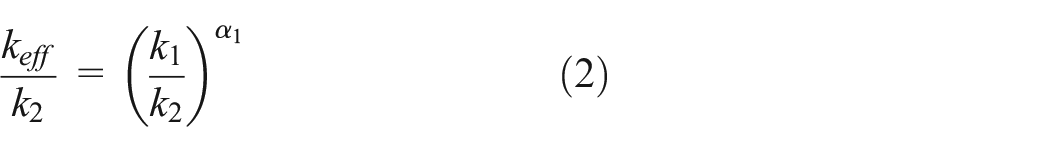
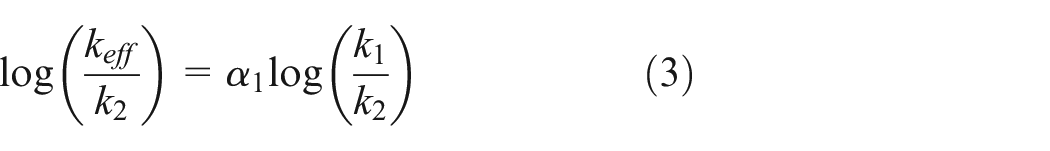
When the phase contrast is small ( $k$  = 10⁻² to 10²) heat flows through both phases and the thermal network exhibits an emergent region in the central region of Figure 2, and the distribution of the phase in the random network has little influence on the thermal conductivity in the emergent area. All the random thermal network models tend to have the same variation in this region. In the emergent region, the contrast between the two phases ( $k$  =  $k_1$ / $k_2$ ) is relatively low ( $k_1$ / $k_2$ ∼ 10⁻² to 10²), and heat tends to flow through both phases. This can be seen in thermal flux diagrams for the range of contrast values, as shown in the results in Figure 3(b) to (i). Since both phases contribute to the effective thermal conductivity of the network, the dependence of the effective thermal conductivity on the network arrangement is small. In the emergent region, a logarithmic mixing rule can be used to describe the effective thermal conductivity ( $k_{\mathrm{eff}}$ ) of the network,

$$k_{\mathrm{eff}}={k_1}^{{\alpha }_1}{k_2}^{1-{\alpha }_1}$$

(1)

Figure 3.

Heat flux for network for a variety of $k_1$ / $k_2$ ratios: (a) $k_1$ (purple), k₂ (blue), (b) $k_1$  =  $k_2$ /10,000, (c) $k_1$  =  $k_2$ /1000, (d) $k_1$  =  $k_2$ /100, (e) $k_1$  =  $k_2$ /10, (f) $k_1$  =  $k_2$ , (g) $k_1$  = 10 $k_2$ , (h) $k_1$ = 100 $k_2$ , and (i) $k_1$  = 1000 $k_2$ .

Dividing equation (1) by $k_2$ gives rise to

$$\frac{k_{\mathrm{eff}}}{k_2}={\left(\frac{k_1}{k_2}\right)}^{{\alpha }_1}$$

(2)

Take the log of equation (2) to

$$\log \left(\frac{k_{\mathrm{eff}}}{k_2}\right)={\alpha }_1\log \left(\frac{k_1}{k_2}\right)$$

(3)

From equation (3), the gradient of log ( $k_{\mathrm{eff}}$ / $k_2$ ) versus log ( $k_1$ / $k_2$ ), as shown Figure 2, should equal the volume fraction of material with thermal conductivity $k_1$ (namely ${\alpha }_1$ ). Figure 2 shows that there is good agreement between the slope of the emergent region in the center of Figure 2 and the volume fraction $k_1$ . Equation (3) is still suitable to predict the effective thermal conductivity of multi-phase heterogeneous material.

These two responses at high and low contrast are likely to occur at ${\alpha }_1$  =  ${\alpha }_2$  = 0.25 since both phases are likely to be percolated, since the percolation threshold for a three-dimensional system is 0.25; this is in contrast to a two-dimensional network where the percolation threshold is 0.5.

Since the three-dimensional heat flow paths are in the interior and cannot be visibly observed, the heat percolation paths are visually analyzed in a two-dimensional network based on a two-dimensional analysis of the stochastic model of the thermal network.

It can be seen in Figure 2 that when there is a high contrast in thermal conductivity (high or low $k_1$ / $k_2$ ) in the network, the thermal conductivity of the variability in the response of individual networks of the same composition, see the left- or right-hand side of Figure 2. At these high contrast conditions, heat flow tends to percolate through the most conductive phase, and the percolation path changes the way the two phases interoperate, which in turn changes the system thermal conductivity. For example, when $k_1$  >>  $k_2$ and $k_1$ / $k_2$ is high, the heat will preferentially flow through $k_1$ , this is clearly evident in Figure 3(b) and (c); when $k_1$  <<  $k_2$ and $k_1$ / $k_2$ is low, the heat will preferentially flow through $k_2$ ; this is clearly evident in Figure 3(i).

Analysis of the results of the thermal network with α₁ = 0.8

The thermal network output for 12 realizations of the random network with ${\alpha }_1$  = 0.8 are shown in Figure 4, namely ${\alpha }_1$  = 0.8 and ${\alpha }_2$  = 0.2. The thermal network output for 12 realizations of the random network with ${\alpha }_1$  = 0.8 is shown in Figure 4. Percolation occurs when the $k_1$ phase (purple) are interconnected across the three-dimensional network. For $k_2$ , the volume fraction is small ( ${\alpha }_2$  = 0.2) and below the percolation threshold, therefore the possibility of a percolated interconnection across the network is small; as result percolation does not occur. For networks where percolation occurs, since the $k_1$ regions are highly interconnected, when $k_1$ → 0 and $k_1$  <<  $k_2$ (see left-hand side of Figure 4), the network thermal conductivity approaches zero. When $k_1$  >>  $k_2$ and $k_1$ →∞ the thermal conductivity of the three-dimensional network also approaches infinity, corresponding to right-hand side of Figure 4. In the central emergent region, there is a similar variation between 12 independent random thermal network models; this is a result of heat flowing through both phases in this low contrast region. There is also a good correlation between the slope of the network response with ${\alpha }_1$ in the central region, and good agreement with the logarithmic mixing rule of equation (1).

Figure 4.

Log-log plot of effective conductivity as a function of $k_1$ / $k_2$ for 12 different randomizations, where ${\alpha }_1$  = 0.8.

Analysis of the results of the thermal network with ${\alpha }_1$  = 0.2

The thermal network output for 12 realizations of the random network with ${\alpha }_1$  = 0.2 are shown in Figure 5. The thermal network output for 12 realizations of the random network with ${\alpha }_1$  = 0.2 is shown in Figure 5. Percolation occurs when $k_2$ phase (blue) is interconnected across the three-dimensional network. For $k_1$ , the volume fraction is small, therefore the possibility of interconnections is small, and the percolation does not occur. For networks where percolation of phase 2 occurs when $k_1$  <<  $k_2$ , the $k_1$ regions act to limit heat flow and the network value approaches a constant value (left-hand side Figure 5), where the limiting value is dependent on the percolation paths and percolation range of $k_2$ ; for example for more tortuous percolation phases of phase 2 the limit conductivity may be low while for more direct percolation paths across the network the limit conduit can be higher. For networks without percolation of k₂, when $k_1$ →0 and $k_1$  <<  $k_2$ (left-hand side of Figure 5), the thermal conductivity approaches zero. When $k_1$  >>  $k_2$ and $k_1$ / $k_2$ is high, the effective thermal conductivity of the network approaches another larger constant value (right-hand side in Figure 5) and approaches a limiting value since there is no percolation of phase 1.

Figure 5.

Log-log plot of effective conductivity as a function of $k_1$ / $k_2$ for 12 different randomizations, where ${\alpha }_1$  = 0.2.

In the central emergent region, there is a similar variation between 12 independent random thermal network models. In the central emergent region, the network response is less dependent on the distribution of phases in the network, as heat is able to flow through both $k_1$ and $k_2$ regions in a similar manner as in Figure 3(e) to (g). This is also a good correlation between the slope of the network response with ${\alpha }_1$ , with good agreement with the predicted value from equation (1).

Summary of thermal response of thermal networks

Figure 6 summarizes the typical response of the three-dimensional thermal networks in the range of ${\alpha }_1$  = 0.1–0.9. At an extreme contrast of thermal conductivity when $k_1$ / $k_2$  < 10⁻² or $k_1$ / $k_2$  > 10², the gradient becomes zero or one, since the thermal conduction is controlled by the series or parallel rules and the exact nature of the zero and one gradient depends on the presence of percolation, or not. Under these high contrast conditions, individual networks with the same components are highly sensitive to the way the components are distributed in the network and presence, or lack, of percolation paths.

Figure 6.

Summary of typical thermal network responses for range of fractions of $k_1$ ( ${\alpha }_1$  = 0.1–0.9).

When the contrast in the two-phase thermal conductivity is moderate, the thermal network showed an emergent response, with a gradient between 0 and 1. In the emergent region, this also a good correlation between the slope of the network response with ${\alpha }_1$ , as is predicted by equation (1).

By comparing the effective thermal conductivity variation of the two-dimensional ¹⁴ and three-dimensional thermal networks, the responses have the similar law as follows:

• (1) In the case of extreme thermal conductivity, the response gradient of the effective thermal conductivity is 0 or 1, which will lead more percolation phenomenon.

• (2) In the middle emergent region, the response gradient gradually increases with increasing ${\alpha }_1$ . There is a good agreement between the slope and the volume fraction ${\alpha }_1$ .

The responses of the two-dimensional and three-dimensional thermal networks also have different properties: the volume fraction of percolation occurring is not the same, and the percolation thresholds are not the same.

Comparison of experimental data with porous materials

While good agreement between the logarithmic mixing rule and the thermal networks is observed, it is of interest to compare the mixing rule with experimental data on real three-dimensional materials.^15–19 For a porous material that has its pores filled with a fluid, $k_s$ is the solid phase thermal conductivity of the porous material, and $k_f$ is the fluid phase thermal conductivity of the porous material.

As can be seen from the Figure 7, for porous media materials, when the contrast between solid phase and flow phase is relatively low, namely $k_s$ / $k_f$ ∼ 10⁻² to 10², the slope of the logarithmic curve is equal to the volume fraction of solid phase, that is, the logarithmic mixing rule is valid and the emergent behavior in porous materials is verified, and the correctness of logarithmic mixing rule in porous materials is also verified. This is further evidence that the emergent behavior of two-phase heterogeneous materials exists, and the logarithmic mixing rule can be used to predict the thermal conductivity of the system in the emergent region.

Figure 7.

Comparison of logarithmic mixing rule with experimental data: (a) porous materials and (b) two-phase systems of ellipsoidal particles.

Construction of three-phase thermal network model

The three-phase thermal network model is shown in Figure 8. The network is composed of three different materials based on 30 30 array, the thermal conductivity of these three materials is $k_1$ (blue phase), $k_2$ (purple phase), and $k_3$ (red phase) respectively. Where $k_1$ is 1, $k_2$ and $k_3$ change from 10⁻⁴ to 10⁴ $\mathrm{W}/(m·K)$ , ${\alpha }_1$ , ${\alpha }_2$ , and ${\alpha }_3$ are volume fractions of three phases respectively, ${\alpha }_1$ +  ${\alpha }_2$  +  ${\alpha }_3$  = 1, ${\alpha }_2$  =  ${\alpha }_3$ . The application of boundary conditions is the same as that of the three-dimensional thermal network above.

Figure 8.

Three-phase thermal network model.

For different volume fractions ( ${\alpha }_1$  = 0.3, 0.5, 0.7), 10 different random thermal networks are studied to explore the changes of effective thermal conductivity caused by different spatial distribution, volume fraction, and thermal conductivity ratio of three phases.

According to the effective thermal conductivity prediction model of heterogeneous materials in equation (1), if the three-phase thermal network also has an emergent region, the effective thermal conductivity of the emergent region is:

$$k_{\mathrm{eff}}={k_1}^{1-{\alpha }_2-{\alpha }_3}{k_2}^{{\alpha }_2}{k_3}^{{\alpha }_3}$$

(4)

Taking logarithm:

$$\log \left(\frac{k_{\mathrm{eff}}}{k_1}\right)={\alpha }_2\log \left(\frac{k_2}{k_1}\right)+{\alpha }_3\log \left(\frac{k_3}{k_1}\right)$$

(5)

Equation (5) predicts the effective thermal conductivity of three-phase heterogeneous materials to a certain extent. Equation (5) can be simplified as $z=\mathrm{ax}+\mathrm{by}$ , and then it becomes a surface problem.

Results and discussion for three-phase thermal networks

Analysis of the results of the three-phase thermal network with α₁ = 0.5

Figure 9 shows the corresponding analysis results of 10 three-phase random thermal network models at ${\alpha }_1$  = 0.5, As shown in Figure 9, percolation occurs mainly in the case of large thermal conductivity difference, namely $k_2$ / $k_1>>$ 10², $k_2$ / $k_1<<$ 10⁻², $k_3$ / $k_1>>$ 10², and $k_3$ / $k_1<<$ 10⁻² of these four cases, heat flux is more sensitive to the spatial distribution and connectivity of the phase, percolation occurs in the thermal network, and three phases can occur percolation respectively.

Figure 9.

Log-log plot of effective conductivity as a function of $k_1$ / $k_2$ for 10 different randomizations, where ${\alpha }_1$  = 0.5.

However, in the middle region, the thermal conductivity of the three phases is similar, and the heat flux flows through the three phases more uniformly, this area is called the emergent region. In the emergent region, equation (5) is valid and can be used to calculate and predict the effective thermal conductivity of three-phase heterogeneous materials. The percolation threshold of two-dimensional three-phase thermal network is 0.5. In the emergent region, the responses of 10 random thermal networks pass through the same plane $z=\mathrm{ax}+\mathrm{by}$ . It can be seen from the Figure 9, and a =  ${\alpha }_2$  = 0.25, b =  ${\alpha }_3$  = 0.25.

Analysis of the results of the three-phase thermal network with α₁ = 1/3

Figure 10 shows the corresponding analysis results of 10 three-phase random thermal networks with ${\alpha }_1$  = 1/3. As shown in Figure 10, when $k_2$ and $k_3$ are large, $k_2$ and $k_3$ dominate the two-dimensional three-phase thermal network, and the effective thermal conductivity of the whole system also increases. In other words, the heat flux tends to flow through the second phase and the third phase, and less through the first phase, namely percolation occurs in the second and third phases. It can be seen from the Figure 10 that when the contrast of $k_1$ with $k_2$ and $k_3$ is high, the distribution has a large influence on the thermal conductivity of the system. For example, percolation phenomenon occurs on the right side of Figure 10. When $k_1<<k_2$ and $k_1<<k_3$ , the heat flux of the random heat network is more inclined to flow through the second and third phases, so that percolation occurs in the second and third phases.

Figure 10.

Log-log plot of effective conductivity as a function of $k_1$ / $k_2$ for 10 different randomizations, where ${\alpha }_1$  = 1/3.

With an increase in $k_2$ and $k_3$ , the effective thermal conductivity of system also increases. There is no percolation in some random thermal networks, so when ${\alpha }_1$  = 1/3, the percolation is mainly determined by the volume fraction of the phase. There is also an emergent region. As shown in the Figure 10, the region with the same variation trend for individual networks with intermedi-ate effective thermal conductivity is called the emergent region. In the figure, the responses of 10 random thermal networks pass through the same plane $z=\mathrm{ax}+\mathrm{by}$ , where a =  ${\alpha }_2$ , b =  ${\alpha }_3$ , equation (5) is correct.

Analysis of the results of the three-phase thermal network with α₁ = 0.7

Figure 11 shows the corresponding analysis results of 10 three-phase random thermal networks with ${\alpha }_1$  = 0.7. Since the percolation threshold of two-dimensional three-phase heat network is 0.5 < 0.7, the first phase has a strong connectivity and the heat flux is passes easily through this phase, so the first phase is more prone to percolate. At this time, the phase distribution no longer plays a decisive role, but the volume fraction dominates, and ${\alpha }_1$ is large. Therefore, the second and third phases do not percolate, and the effective thermal conductivity of the system does not increase with the increase of $k_2$ and $k_3$ . Percolation of the first phase occurs when $k_1>>k_2$ and $k_1>>k_3$ , In the figure, the responses of 10 random thermal networks pass through the same plane $z=\mathrm{ax}+\mathrm{by}$ , where a =  ${\alpha }_2$ , b =  ${\alpha }_3$ , equation (5) is correct.

Figure 11.

Log-log plot of effective conductivity as a function of $k_1$ / $k_2$ for 10 different randomizations, where ${\alpha }_1$  = 0.7.

Conclusions

This paper studies the thermal conduction characteristics of three-dimensional and three-phase thermal networks, analyzes the emergent behavior of the heat network and the thermal conduction characteristics of heterogeneous materials. Some useful results are obtained as follows.

• (1) At conditions of high phase contrast in thermal conductivity of the phases in thermal networks, the effective thermal conductivity of the same component thermal networks exhibits greater variability and is sensitive to the way the components are distributed within the network.

• (2) When the contrast between the thermal conductivities of the phases in thermal networks is small, there is no preference in the flow path of the heat flow, which flows relatively uniformly through both phases, with a constant gradient of the thermal network response.

• (3) For two-phase thermally conductive heterogeneous materials, the effective thermal conductivity of the emergent region can be predicted using the logarithmic mixing rule, thus providing a fast and easy method for predicting the thermal properties of the material.

• (4) Percolation occurs separately in each phase of three-phase systems. Similar to the two-phase system, three-dimensional heterogeneous materials also have an emergent region. The effective thermal conductivity of the emergent region can be predicted by using the logarithmic mixing rule, and the percolation phenomenon occurs outside the emergent region.

• (5) The percolation threshold of two-dimensional thermal network system is 0.5 and that of three-dimensional thermal network system is 0.25.

Using the emergent behavior and logarithmic mixing rule for thermal conduction in heterogeneous materials can provide guidance for the future development of multiphase systems.