Parallel simulation of high-speed trains controlled by radio block centers using Spark cloud

Abstract

Train movement prediction simulation is an effective method of enhancing operation safety and efficiency of railway transportation. Train movement data generated by the trains running in a railway network are huge, and on the other hand, the data quantity generated from data processing is also explosively increased for the analysis and decision such as conflict recognition and scheduling optimization, which greatly increases the time cost of prediction simulation. This paper attempts to propose a train movement model driven by the movement authorities (MAs) issued from radio block centers (RBCs) and its parallel simulation algorithm realized on Spark cloud. This paper provides a solution of iterative computing of dynamic process simulation based on cloud. Different from the general big data processing of independent datasets, the resilient distributed datasets are expandable along iterative computing processes. The Dataframe of SparkSQL modules on Apache Spark is employed to handle the problems of usage interdependency of datasets. The parallel simulation is realized by Scala language that is used to build the Spark platform. The simulation results on a high-speed railway network demonstrates that the proposed train movement model and parallel algorithm can achieve theoretical rationality and decrease the time cost to satisfy real-time performance.

Introduction

Operation efficiency and safety are the core disciplines of railway traffic. Many advanced control systems have emerged in the railway transportation industry to keep trains run in a secure environment, such as communication-based train control system (CBTC) and radio block center (RBC)-based train control system (RBC-TCS). Pascoe and Eichorn ¹ introduced the concept of CBTC and how it works, and the CBTC system was compared with other traditional train control systems from the structures, functions, and working principles. Ranjbar et al. ² represented the characters of European Train Control System Level 2 (ETCS L2), hybrid level 3 (ETCS HL3), and analyzed the impacts of typical signaling systems on transport capacity. In the RBC-TCS such as Chinese Train Control System – Level 3 (CTCS-3), train movements pursuing a speed of 350 km/h are controlled by the movement authorities (MAs), which are generated by RBCs. The running trains feedback their running states including real-time speeds and positions to the RBCs, and the RBCs send control orders to the trains after analyzing the train real-time data. While, the analyses are mainly confined to the safety and logic check, and the prediction and optimization are not involved so much for the MA granting. Because the information processing of all trains in a high-speed railway network will be subject to a large number of computing burdens, this study attempts to address the parallel prediction simulation of high-speed train operations on Spark cloud, so as to enhance train movement safety, generate more feasible train scheduling decisions, and make the whole railway network operate more efficiently.

The train movement model is the core component of train movement prediction simulation. The cellular automaton (CA) is a kind of model to replicate self-organization and self-evolvement systems. Nagel and Schreckenberg ³ proposed the Nasch model to represent stochastic traffic flow, using the basic rules of speed and position updates to reproduce the main characteristics of realistic traffic. The CA model has also been applied to represent railway traffic. Li et al. ⁴ and Ning et al. ⁵ proposed the moving-block and fixed-block train movement models based on the Nasch CA model. The rule-based train movement model was developed for safety justification, utilizing evidence theory and train movement reference models by Zhou et al. ⁶ The method of multi-sensor data fusion based on the transferable belief model was also proposed to recognize train movement situations employing train movement models by Zhou et al. ⁷

In this study, in light of the working mechanism of RBC-TCS, we designed a new train movement model that describes train movements driven by the MAs issued by RBCs. This model extends the current train movement models based on block sections into that based on RBCs, which more tallies with the practical working mechanisms under current high-speed train control architecture. Considering the scale of the whole railway network, train monitoring and control employing train movement prediction will involve huge train data and handling. Parallel computing based on cloud computing has great potentials for big data processing. This study attempts to employ cloud computing to realize the paralleling computing of train movement prediction in the monitoring and control of high-speed trains in a railway network.

Cloud computing has greatly developed and been widely used in various fields since it was proposed in the 1980s. It can offer a powerful computing ability and a large scale of storage space for the analysis and processing of big data. Buyya et al. ⁸ analyzed some research development of could computing in emerging IT platforms from the aspects of 21st century vision of computing, including cluster computing and grid computing, and compared some existing cloud platforms and the markets of global clouds. Armbrust et al. ⁹ listed the characters of cloud computing, compared the cloud computing and conventional computing, and summarized some current opportunities and obstacles of cloud computing. Nowadays, many cloud computing platforms and parallel computing models have been developed. In 2004, Google advanced the MapReduce parallel computing model. ¹⁰ MapReduce is an architecture that is used in parallel computing based on map and reduce operations, which has good scalability and high fault tolerance. MapReduce is easy to program, but it does not perform well in real-time computing and stream computing. Inspired by MapReduce, a Hadoop system was developed. ¹¹ It has the same advantages of MapReduce, but it realizes the distributed file system that endows Hadoop with high reliability and high throughput. In 2009, Apache Spark was born in the AMPLab of UC Berkeley. In terms of the parallel computing models, Spark is similar to MapReduce, thus, it inherits the preponderance of MapReduce. Different from the MapReduce, Spark does well in stream computing and real-time computing, initiating the memory-based computing in distributed computing systems. Zaharia et al. ¹² introduced the functions of Spark from its programming model and libraries, and especially analyzed the basic unit of Spark – resilient distributed datasets (RDDs), which makes the Spark model generalized. In the applications of Spark, based on the characters of Spark which does well in stream computing, Ramirez-Gallego et al. ¹³ designed a neighbor classification algorithm which was used for processing massive and high-speed data streams by Spark. Chen et al. ¹⁴ proposed a parallel random forest algorithm for big data processing on Spark, which optimizes the data-parallel and task-parallel computing, and reduces the data transmission cost. Alfailakawi et al. ¹⁵ presented a parallel implementation method of sine and cosine algorithms on Spark, which improves the performance of solution quality and run time in solving complex optimization problems. Wang et al. presented the Backpropagation-based OnlIne hardware fault Diagnosis System (BOIDS) which is an intermittent fault diagnosis system based on BP neural network method as a diagnosis scheme. They tested BOIDS on a cloud computing simulation environment and the result showed that BOIDS could provide a high diagnosis accuracy of fault location and fault model. ¹⁶ In recent years, the applications of cloud computing to railway industry have aroused increasing attention. Wang et al. designed a general distributed Top-k monitoring algorithm (DTMR) which can support continuous and strictly monotone aggregation function. DTMR was used to process the multiple high-speed rail data streams in the cloud computing environment and its efficiency was proved by the practical data and simulated data. ¹⁷ Xie and Qin ¹⁸ proposed a new detection framework by using Internet of Things for railway perimeter intrusion detection, the results of computational experiments showed their detection framework is effective and can conspicuously increase the detection precision. Laiton-Bonadiez et al. ¹⁹ systematically summarized the application of industry 4.0 technologies to rail transportation industry, which includes big data and cloud computing technologies. Wang et al. ²⁰ proposed a 3D railway intelligent construction system architecture which integrates big data and cloud computing technologies. Gala et al. ²¹ found that the kernel-based virtual machine is fit for deploying a real-time cloud to implement the applications of real-time safety-critical cases in railway industry.

Monitoring and optimizing train movement operations requires train movement simulation and prediction to justify train movement safety and performance, and this inevitably involves a strong big-data processing ability relying on clouding computing. The application of clouding computing to train movement simulation and prediction is an uncultivated field to await remarkable explorations. In this study, a parallel simulation algorithm will be proposed based on Spark Cloud for train movements controlled by the MAs from RBCs. The contributions of this paper are summarized as follows:

1. A train movement model is developed for high-speed railway, addressing radio block sections and speed update rules with one-step forward prediction.

2. A parallel simulation algorithm of train movements in a railway network is proposed and implemented on Spark cloud under the geographically distributed RBC-TCS architecture.

3. A big data processing method is proposed to iteratively deal with train movement information using the Spark native language Scala to achieve a fast execution speed.

The rest of this paper is organized as follows. Section “Train movement model” analyzes the mechanism of RBC-based TCS and develops the corresponding train movement model and algorithm. Section “Parallel simulation of train movement” represents the parallel simulation architecture and algorithm of train movement based on Spark. Section “Simulation results” demonstrates the simulation results and rationalities. The conclusions are drawn in Section “Conclusions.”

Train movement model

MA

MA is the order and permission about the route, distance, and speed that a train can run with. That is, a MA specifies the feasible route, the farthest distance, and the maximum speed that a train can operate during a time period. It is engendered from the RBC using security computers, based on the information collected from the front adjacent train, track circuits, and interlocking facilities. The RBCs are connected with other ground equipment such as scheduling and commanding center, and generate MAs to keep trains run in safe situations. The MA is utilized by the onboard equipment to implement safety-distance control. The onboard equipment compares the train actual speed with the allowable speed in MA in a real-time manner, service braking or emergency braking will be enforced depending on the exceeding degree. As shown in Figure 1, A RBC controls the related en-route trains locating within the same region. When a train runs from region A to region B, it will be controlled from RBC A to RBC B. There exist handover boundaries between RBCs A and B.

Figure 1.

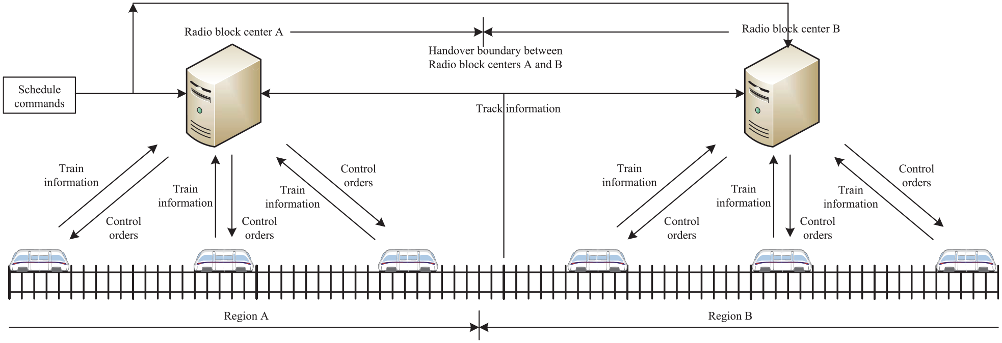
RBC control architecture of high-speed trains.

Train operation mechanism

In the MA, there are two important indicators to ensure a train to run in safety, that is, the allowable operation distance and speed for a valid time period, in short, MA length and speed, defined as L_MA(R) and v_MA(R), respectively, where R represents the currently addressed train. Within each period, the RBCs will collect the information from trains and railway lines, then they will generate complete effective MAs and send them to trains, and the trains will move by following the MA restrictions.

MA length

We define P(x) as the position of point x in a railway line, R _i as the objective train, and R _j as the front adjacent train of R _i . To obtain the MA length of train R _i , we define a point E as the endpoint of MA in case that the MA is valid during the current period. The point E is determined by two points A and B, where A is the point to enter the radio block section which is occupied by R _j , and B is the point where the next station locates. The point which is closer to train R _i will be selected as point E. P(A) and P(B) are the positions of points A and B in a railway line, d_a and d_b represent the distances from train R _i to points A and B, respectively. Figure 2 demonstrates the relationship among these parameters. In this way, the front adjacent trains and stations are represented in a uniform manner.

Figure 2.

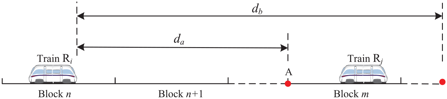
The distances related to movement authority length.

Accordingly, d_a and d_b are formulated as

$$d_a=P(\mathrm{A})-P({\mathrm{R}}_i)$$

(1)

$$d_b=P(\mathrm{B})-P({\mathrm{R}}_i).$$

(2)

The MA length of R _i is the minimum distance of d_a and d_b, represented by

$$L_{\mathrm{MA}}({\mathrm{R}}_i)=min(d_a,d_b).$$

(3)

For safety, the braking distance of train R _i related to its current speed must be less than or equal to L_MA(R _i ) at any time.

MA speed

In the current MA of train R _i , the velocity of R _i cannot exceed a speed limit at any moment, which is defined as the target speed of R _i , or the speed restriction in the MA of R _i , in short, the MA speed. The target speed is determined by the following factors:

1. Maximum speed of train: This is the maximum speed that a train can achieve in design, dependent on the train type. It is defined as v_max.

2. Block-section speed restriction: This speed is decided by the position and status of the radio block section. Different positions of block sections have different speed restrictions, engendering multiple speed limits for a train. It is defined as v_block.

3. Allowable maximum speed: This speed is calculated from the MA length of train R _i . It is the maximum speed that a train can be allowed if the brake distance equals to L_MA(R _i ). It is defined as v_s.

Figure 3 depicts the relationship among these three speeds. In practice, the MA speed might not detail these three speeds, but they are indispensable for train movement description. The minimum of the above speed limits is the target speed of train R _i , which is the maximum speed that train R _i can reach in its current MA, formulated as

$$v_{\mathrm{MA}}({\mathrm{R}}_i)=min(v_{\max },v_{\mathrm{block}},v_{\mathrm{s}}).$$

(4)

Figure 3.

The speed restrictions related to movement authority speed.

Speed variation mechanism

The speed change of train R _i is controlled by the MA length, MA speed and brake distance. We use two variables AC₁ and AC₂ to express the speed change tendency of train R _i at instants t and t + 1. If train R _i need not decelerate at instant t, then AC₁ = 1, otherwise AC₁ = 0. Based on the calculation of train R _i movement at instant t, if the speed need not be decreased at next instant t + 1, then AC₂ = 1, otherwise AC₂ = 0.

We define v_t as the speed of train R _i at instant t, v_t + 1 as the speed at instant t + 1, d_t as the brake distance of speed v_t, and d_t + 1 as the brake distance of speed v_t + 1. The acceleration and deceleration at instant t are denoted as a_t and b_t, respectively. We presume the temporarily predicted speed of R _i is $v{\prime }_{t+1}$ at instant t + 1, the corresponding brake distance is $d{\prime }_{t+1}$ , and the MA length is L_MA(R _i )- $v{\prime }_{t+1}$ at instant t + 1. The relationship between speed and brake distance can be approximately formulated as follows:

$$d_t=v_t^2/2b_t$$

(5)

$$d{\prime }_{t+1}=v{\prime }_{t+1}^2/2b_{t+1},$$

(6)

where,

$$v{\prime }_{t+1}=v_t+a_t·A{C}_1.$$

(7)

It should be noted that, if a_t is numerically represented in unit time, it is numerically equal to the result that a_t is multiplied by the unit time, so the unit time can be omitted in equation (7). This is similar to the CA description in Nagel and Schreckenberg. ³

We can acquire the values of AC₁ and AC₂ decided by the MA length and brake distance in the following ways:

$$A{C}_1=\{\begin{array}{c}0,L_{\mathrm{MA}}({\mathrm{R}}_i)<d_t\hfill \\ \multicolumn{1}{c}{1,L_{\mathrm{MA}}({\mathrm{R}}_i)\ge d_t}\end{array}$$

(8)

$$\begin{array}{c}\multicolumn{1}{c}{A{C}_2=\{\begin{array}{c}0,L_{\mathrm{MA}}({\mathrm{R}}_i)-{v\prime }_{t+1}<{d\prime }_{t+1}\hfill \\ \multicolumn{1}{c}{A{C}_1·1,L_{\mathrm{MA}}({\mathrm{R}}_i)-{v\prime }_{t+1}\ge {d\prime }_{t+1}}\end{array}}\end{array}$$

(9)

Similarly, if $v{\prime }_{t+1}$ is numerically represented in unit time, which is numerically equal to the result that $v{\prime }_{t+1}$ is multiplied by the unit time, so the unit time is also omitted in equation (9).

Speed and position update algorithm

If there exist only acceleration and deceleration processes without one-step forward prediction in the train movement description, it will cause intense train speed fluctuations, which deviate from the practical cases, and will be substantially unfavorable to the comfortableness of passengers if being regarded as control objectives. For the sake of safe and stable operations of trains, we introduce AC₁ and AC₂ to describe the speed update rules, that is, acceleration and deceleration behaviors with one-step forward prediction. In this way, the periodic speed oscillations between accelerations and decelerations can be prevented, which are incurred by model imperfections themselves beyond practical requirements of accelerations and decelerations. We define x_t and x_t + 1 to indicate the position of train R _i at instants t and t + 1. The position update of train movement is based on the newly updated speed.^4,5 The speed and position updates of train movement is described in Algorithm 1.

Algorithm 1: Speed and position updates algorithm of train movement.

Input: Speed $v_t$ of train R i at instant t, MA length $L_{\mathrm{MA}}({\mathrm{R}}_i)$ , MA speed $v_{\mathrm{MA}}({\mathrm{R}}_i)$ , accelerations $a_t$ and decelerations $b_t$ related to different speeds. Output: Speed and position at next instant t + 1. 1: Configure AC1 and AC2 according to equations (5)–(9). 2: if $v_t>v_{\mathrm{MA}}({\mathrm{R}}_i)$ 3:   $v_{t+1}=max(v_t-b_t,0)$ 4: else if $v_t=v_{\mathrm{MA}}({\mathrm{R}}_i)$ 5:  if $A{C}_1=1$ 6:    $v_{t+1}=v_t$ 7:  else 8:    $v_{t+1}=max(v_t-b_t,0)$ 9:  end if 10: else 11:  if $A{C}_1=1$ 12:   if $A{C}_2=1$ 13:     $v_{t+1}=min(v_t+a_t,v_{\mathrm{MA}}({\mathrm{R}}_i))$ 14:   else 15:     $v_{t+1}=v_t$ 16:   end if 17:  else 18:   if $v_t>b_t$ 19:     $v_{t+1}=min(v_t-b_t,L_{\mathrm{MA}}({\mathrm{R}}_i))$ 20:   else 21:     $v_{t+1}=L_{\mathrm{MA}}({\mathrm{R}}_i)$ 22:   end if 23:  end if 24: end if 25:  $x_{t+1}=x_t+v_{t+1}$

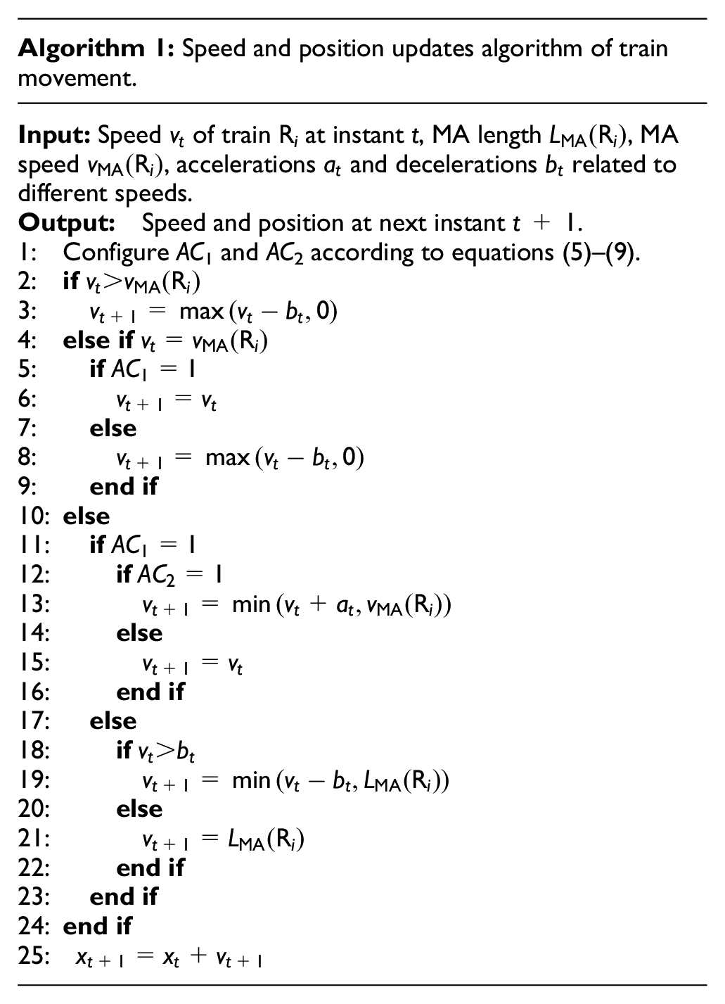
In Algorithm 1, at first AC₁ and AC₂ are calculated according to equations (5)–(9). And then, train R _i judges if its speed exceeds the MA speed. If so, the deceleration will be enforced onto train R _i , as lines 2 and 3 indicate. If the speed is equal to the MA speed, speed holding or deceleration will be implemented, as lines 4–9 describe. Lines 10–24 represent that, if AC₁ = 1, train R _i either accelerates or maintains its current speed, which is determined by AC₂ = 1 or 0; otherwise, train R _i will decelerate with an appropriate deceleration.

Parallel simulation of train movement

Parallel computing architecture

Apache Spark is a big data processing engine that was developed by the UC Berkeley AMPLab. The Spark architecture is composed of a driver and several executors. In actual applications, a complete Spark cluster contains a master node and multiple worker nodes. The driver belongs to the master node, executors belong to worker nodes, and a worker node can deploy plural executors. Figure 4 demonstrates the parallel computing architecture on the Spark cloud, which reveals the relationship between the driver and the executors. The driver analyzes the applications that users submit and generates a directed acyclic graph. Then, the driver will divide the applications into several stages, and each stage includes multiple tasks which will be scheduled to the executors to perform. In this way, the executors can process the tasks in the same stage to realize the purpose of parallel computing.

Figure 4.

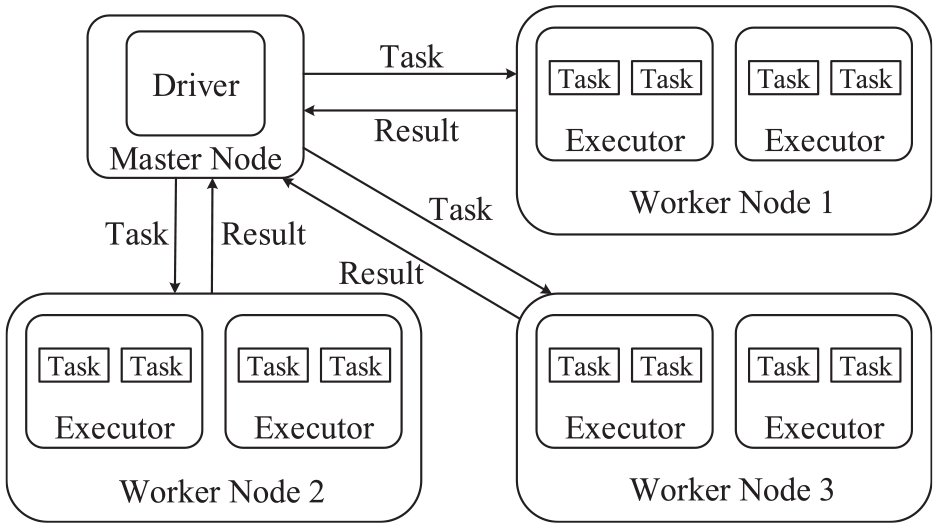
Parallel computing architecture on Spark cloud.

A core of Spark is the Resilient Distributed Dataset (RDD), which is the basic unit for any action of parallel computing on Spark. The RDD has resilient, distributed, read-only, and creation features suitable for big data processing. The resilience makes the RDD can save data adaptively. By default, the RDD is stored in RAM, which endues Spark with a high-speed calculation capability. When there is not enough space in RAM, Spark will store the RDD on hard disks. In Spark, the RDD is divided into partitions and stored at different computing nodes. Every partition of a same RDD will be carried out by a same program simultaneously, which brings Spark the ability of parallel computing. The characters of read-only and creation provide Spark with the ability of fault tolerance. If there is a partition lost at a node, Spark will recalculate the partition from its parent RDD to recover the whole computation.

The operations on RDDs can be summarized into two categories, that is, transformations and actions. The transformation creates a new RDD from an existing one. But they are lazy operations because they do not immediately work out results and just record these operations need being applied to some RDDs. The action will return values to the driver which are the calculation results on RDDs. The transformations are computed only when the actions are triggered, and then, they will calculate results and return them to the driver. When an application is submitted to the driver, it will engender a directed acyclic graph according to the transformations in the application after the actions are triggered, and subsequently, the driver will schedule executing the tasks of the graph. The operation mechanism on RDDs is illustrated in Figure 5. In Figure 5, blocks A to I represent different RDDs, and the little blocks in them denote data. The operations such as map, union, join, reduceByKey, and groupByKey are the transformations, but saveAsTextFile is the action. A, B, and D are the initial RDDs, and they are created from raw data. C, E, F, and G are the child RDDs, and they are created by transformations from the initial RDDs. I is the RDD providing the final results of the entire application, which will be returned to the driver by actions. Stages 1, 2, and 3 are the different stages that are partitioned by the directed acyclic graph.

Figure 5.

Operations on RDDs.

Parallel simulation

Computing architecture

Train movement simulation prediction plays a crucial role in the conflict prediction and scheduling optimization, which involves great computing burden. Train movement prediction information constructs the RDD for parallel computing. The RDD is decomposed into some partitions, with each partition addressing the movements of a definite number of trains on railway lines. In the common big data processing, the RDD is fixed, and the datasets being decomposed into are mutually independent and separately handled by worker nodes. Different from these aspects, the RDD in this study is expanded with time, and the data handled by a worker node may come from some datasets at different partitions, which brings operation complexity for parallel iterative computing.

Train movement information contains time, speed, position, and train states such as move or not, dwell at a station or not, and adjacent train number. Since train movement information will be iteratively updated with time, we adopt SparkSQL to process train movement information for convenience, which is a module for working with structured data of Spark. Dataframe is a kind of RDD with a schema to distinguish the different properties and meanings of data, so Dataframe is employed to store the train information. Comparing with the other RDDs, Dataframe has a higher computing speed and is better at handling structured data. Dataframe imports schema to the data structure such that Spark can handle the data that needs calculating by controlling the schema, which makes the operations on big data more concise and convenient.

Train movement data construction and handling are illustrated in Figure 6. The train movement RDD is handled by calling the schema. The data is cut into multiple partitions and respectively stored at different worker nodes in the form of Dataframe. In each simulation cycle, the data will be calculated by executors at the same time and recorded after all executors have accomplished their computing tasks. However, before being recorded, the data in the form of Dataframe should be converted into arrays which will be converted into the variables capable of being added to Dataframes. When train movement is predicted in prediction horizon P, the Dataframes are expanded with time. In each unit-time step, train movement calculations are performed using some worker nodes to deal with the datasets sequentially partitioned according to train number. In this way, many expandable datasets can be accessed by a worker node, especially when the front adjacent train movement information locates at other worker node.

Figure 6.

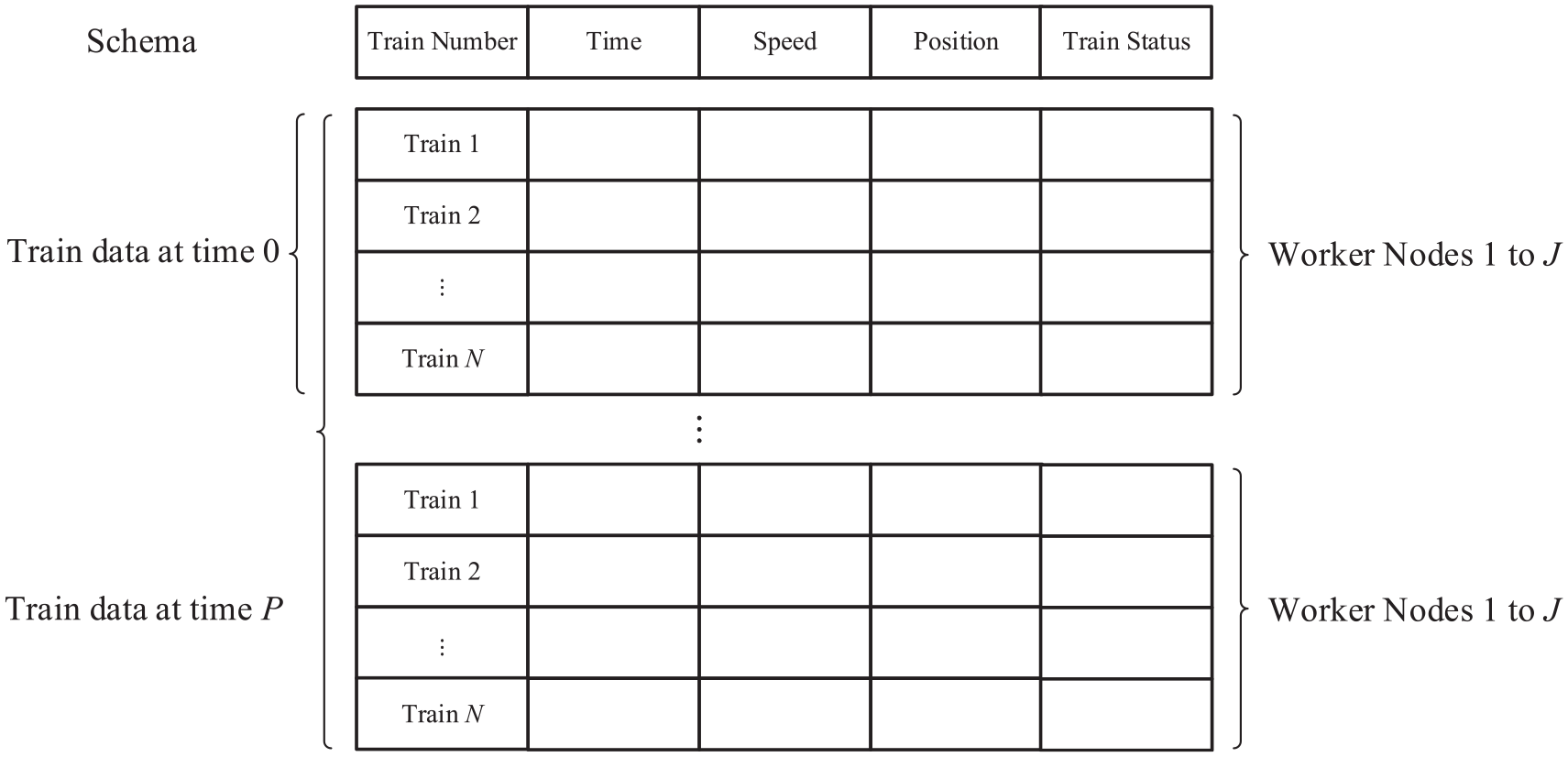
Train movement data construction and handling.

Algorithm description

The processes of train movement parallel simulation are described in Algorithm 2, including initialization, parallel computing, and result submission. Line 1 represents the initialization processes, lines 2–30 elaborates the parallel computing processes, and line 31 indicates the result submission.

Algorithm 2: Train movement simulation based on parallel computing architecture.

Input: Number of worker nodes J, number of running trains N, original information of running trains TrainRecord_Origin, and prediction horizon P. Output: Train movement information in prediction horizon P. 1:  Initialize the Spark basic architecture, and send the original information to the master node. Declare and define the train information update functions. Initialize the parameters such as J, N and P. 2: fort = 1 to P do 3:  ift = 1 then 4:   Create Dataframe DF_Train from TrainRecord_Origin. 5:  else 6:   Create Dataframe DF_Train from the record of train information at the last  simulation time step TrainRecord_Time[t−1]. 7:  end if 8:  Divide DF_Train into J partitions DF_Train[1], DF_Train[2], …, and DF_Train[J], and send each partition to a worker node. 9:  parallel forj = 1 to J do 10: for each train of DF_Train[j] 11:  Acquire the information of the front adjacent train such as speed and position. 12:  Acquire the information of the front closest station such as station location, that whether the train needs to stop at the station, and the speed restriction if the  train pass through the station. 13:  Calculate the train speed at the next time step t + 1 according to the above information using Algorithm 1. 14:  if the train arrives at the station but not the terminal 15:   Check the train dwell time at the station and the speed at the next time step. If the dwell time has run out and the speed is not 0, the train can leave the current station; otherwise, it will still stay at the station. 16:  else if the train arrives at the terminal 17:  Remove the train from the railway network, and record all data of the train generated from the simulation. 18:  else (the train is within the block section) 19:   Check its status mark. If the mark is “unmoved,” according to the speed update within a time step, and change the mark into “moved”; otherwise, no action is performed. 20:  end if 21:  end for 22:  Create the new Dataframe DF_UpdateTrain[j] from the updated train information as the result at current simulation step, and send DF_UpdateTrain[j] to the master node. 23: end parallel for 24: Convert the data type of all partitions DF_UpdateTrain[1] to DF_UpdateTrain[J] from Dataframe to arrays, and combine them into one variable UpdateTrainData. 25: ift = 1 then 26:  Add UpdateTrainData to TrainRecord_Origin to form an updated record TrainRecord_Time[1] of train information for the first simulation time step. 27: else 28:  Add UpdateTrainData to TrainRecord_Time[t-1] to form an updated record  TrainRecord_Time[t] of train information for the current simulation time step. 29: end if 30: end for 31: Submit train movement record TrainRecord_Time[P] as the final result to the user.

The initialization processes include cloud computing system initialization and train movement initialization. The Spark session function is adopted to initialize the constructed computing cluster such as master and worker nodes, and also achieve the initialization of Dataframe. The train movement initialization contains the declaration and definition of the functions and parameters, such as speed and position update, train number, and prediction horizon.

Parallel computing processes involve Dataframe construction, parallel computing, and Dataframe update for each time step. Lines 3–8 show the Dataframe construction processes. In the parallel computing processes, at first, data acquisition is performed as lines 11 and 12 outline. That is, each train running in a railway network will find its front adjacent train and acquire its position and speed, find its front closest station and acquire the information about stopping at or passing through that station, and so on. After that, the system will generate the MA for each train based on the information collection before, and send it to each train. Then, the speed and position updates will be performed using Algorithm 1 using the Dataframes locating at worker nodes. Subsequently, according to the train whether at station or at terminal or within block section, the corresponding operations are performed as lines 14–20 state. If the train is at station, it either leaves from the station or continue dwelling at the station based on that if the dwell time has run out or not and the speed is 0 or not. If the train has arrived at the terminal, the train will not appear in the railway network any more, and its movement processes will be recorded. If the train is within the block section, check the train movement status and update it to avoid the repetitive processing. Line 22 points out the information that the worker nodes submit to the master node. Lines 24–29 demonstrate the processes how the newly generated structured data at next time step are added into the Dataframe at the current time step, in which manner, the Dataframes are expanded with time, and the problem is resolved that the RDD should be fixed in the common big data processing.

In the end, as line 31 sketches, after all calculations of the program have been completed, the record TrainRecord_Time[P], which contains the information of each train at each instant in the prediction horizon, will be collected by the master node. At the master node, the record will be saved as a database file such as csv type by the Spark cloud, and the user can download the file by accessing the master node.

Simulation results

Simulation conditions

The simulation conditions include railway network conditions, train conditions, and cloud computing conditions. The railway network consists of eight transverse lines and eight longitudinal lines. The departure interval is set as 3 min. Therefore, in 24 h, the maximum train number is 7680 for one way. In this high-speed railway network, the trains can run at the maximum speed of 350 km/h. In this study, the cloud computing cluster was built on the third-party cloud service by the Alibaba Cloud Computing Corporation. ²² The service provides customers with a large number of nodes to build computing clusters. The Cloud service parameters are shown in Table 1. The simulation program is written by Scala to achieve the highest execution speed, because the Spark cloud platform is developed by Scala.

Table 1.

Cloud service parameters.

	Master node	Worker node
CPU type	Intel Xeon Platinum 8269CY	Intel Xeon Platinum 8269CY
CPU clock frequency	2.5 GHz	2.5 GHz
Number of cores	4	4
RAM	16 GB	16 GB
Band width	1.024 Gbps	1.024 bps
Apache Spark version	Apache Spark 2.4.7

Computing performance and rationality

Figure 7 and Table 2 illustrate the execution times with different number of computing nodes in the cloud computing cluster in the prediction horizon of 300 s. As shown in Figure 7, when the number of computing nodes is no more than 9, the running time of the program decreases substantially with the increase of the node number. When the number of computing nodes is more than 9, with the increase of the number of computing nodes, the program runtime only has a slight change and tends to keep stable. It indicates that the parallelization execution of the program is obviously effective if the scale of the cluster is under nine computing nodes for the simulation case. The variation trend demonstrates that if the scale of the cluster exceeds a quantity, with the time cost of communications increasing between computing nodes, the computing time performance by parallelization will not be ideal. The time cost of parallel computing is composed of multiple aspects, including time costs of computing tasks, communications between nodes, task scheduling, synchronization, and so on. With the increase of computing nodes, if the time cost of computing tasks reduced by computing nodes are roughly compensated by those increased by other aspects, the total computing time tends to be stable. However, if not so, the total computing time may increase as the cases with computing nodes 8, 10, 11, 14, and 16. From Table 2, it can be found that the minimum runtime case of the program execution is that the cluster employs nine computing nodes, and the time consumption is 186,845 ms. This time takes 62.3% of the entire prediction horizon, which demonstrates that the proposed parallel algorithm can achieve the task of real-time train movement simulation in the prediction horizon, because within the prediction horizon, the simulation can be accomplished for conflict discovery and scheduling optimization.

Figure 7.

The execution times of the program under different node numbers.

Table 2.

The computing efficiency of the cluster with different number of computing nodes.

Number of computing nodes	Execution time of the program (ms)
2	504 869
3	303 059
4	256 219
5	216 544
6	212 015
7	190 693
8	196 974
9	186 845
10	196 518
11	211 083
12	199 075
13	191 391
14	194 792
15	190 613
16	197 824

Figure 8 illustrates the relationship between the braking distance and the initial speed of braking for one kind of high-speed trains. Based on the braking-distance curve in Figures 8 and 9 demonstrates the time-position relationships of a part of trains in case of different departure times such as 60, 120, and 180 s. As shown in Figure 9(a) to (c), when the departure interval is short, the speed changes have great fluctuations. But along with the increase of the departure interval, the fluctuations tend to be not so extensive. These processes indicate that, when the departure interval is short, the MA distances that the later trains acquire will also become short, and correspondingly, the reaction spaces of the later trains will become small. In this situation, the later trains will be more sensitive to the speed changes of their ahead trains. From Figure 9(a) to (c), it can also be found that there exist no coincidence points in the train running trajectories except at the stations with platforms accommodating more trains. This indicates that there is no conflict happening to trains. Further, the following phenomena between trains imply that no train moves beyond the MA constraints. When trains leave from stations or run toward stations, they will accelerate or decelerate smoothly and stably, and no sudden or abnormal speed changes occur. The rational results can be achieved using the parallel simulation program, which accounts for that the MA granting, train speed and position updates, as well as the Dataframe construction, worker node computing, and master node handling are correct.

Figure 8.

The braking-distance curve under different initial braking speeds of a train.

Figure 9.

Time-position tracking of a part of trains in the network: (a) 60-s departure interval, (b) 120-s departure interval, and (c) 180-s departure interval.

Conclusions

Cloud computing is a powerful measure to realize train movement prediction, and management and control of high-speed railway networks. In this study, we have proposed the train movement model based on the MAs issued by RBCs and the parallel computing algorithm which is realized on the Spark cloud platform. The simulation results demonstrate that the time cost is huge for the prediction of the movements of all trains in a railway network, and the parallel algorithm realized on the Spark cloud can effectively reduce the time cost. The advantage at the time cost makes more trains in a railway network can be predicted at the same time, and more complex and massive calculations and functions combined with the train movement prediction can be accomplished in a real-time manner. Indeed, Spark initiates memory-based computing, which has made a progress for scientific iterative and real-time computing based on clouds, but the applications about that, a computing node can employ multiple expandable datasets, require indirect ways to realize. This study provides a solution to realize iterative and real-time computing using Spark cloud, to overcome the limitations of common applications that, one computing node only employs a fixed dataset in the current cloud-based big-data processing architecture. Spark cloud is an advanced distributed computing platform with high efficiency and easy accessibility. With the advancement of clouding computing, the applications of clouding computing to railway industry will become pervasive, and the parallel simulation and prediction of train movements will provide a support for real-time train operation optimization.