Sage Journals: Discover world-class research

Abstract

The sensitivity analysis model is frequently used to express the influence of conditional elements on structural reliability. However, the traditional sensitivity analysis model is limited to a few influencing factors, and has a small scope of application. In this paper, a modified sensitivity model is proposed by combining the optimal polynomial response surface function with the Sobol sensitivity algorithm. And the sensitivity calculation approach was combined with coupling factor test design, range verification, multi-body dynamics analysis and structural statics analysis, which enables to achieve the quantitative sensitivity value of the influence of conditional factors on structural reliability. Finally, a typical harvester structure is selected as a case, to verify the evaluation accuracy and effectiveness of the revised model. The results show that the sensitivity of threshing drum speed has the greatest influence, while the sensitivity of granary load has the least influence. The average quantitative prediction accuracy of revised approach is up to 97.36%. The revised model can accurately evaluate the sensitivity value of coupled influencing factors for industrial equipment.

Keywords

Multiple coupling factors sensitivity model response surface function reliability working conditions

Introduction

The operation safety assessment of large mechanical equipment has gradually become an important link in the maintenance process, which is developing toward lightweight structure, uninterrupted operation and real time monitoring.^1–3 Small damage may cause great harm to the equipment operation safety, with the working time increasing.^4,5 At the same time, the combined effect of external random factors and operating condition parameters will directly affect the damage process,⁶ and become an important factor affecting the operation safety of equipment.^7,8 Therefore, quantitatively evaluate the relationship between influencing factors and structure reliability indicators is very important for further ensure the operation safety of equipment, which has become the research focus in the field of reliability.^9,10 However, for industrial applications, there will also be internal coupling effect between the influencing factors, which will have a composite impact on the reliability index.^11,12 Comparing with the influence of a single factor, the combination of multiple factors is more harmful to the equipment safety.^13–16 For the reliability optimization of turbine blisk structure, Zhang et al.¹⁷ considered the relation between the comprehensive reliability indicators and working conditions. Zhu¹⁸ developed a hybrid iterative conjugate first-order reliability method for fuzzy reliability analysis (FRA) of the stiffened panels. Taking the dynamical mechanical parameters as the reference condition and considering the influence of other conditions, the measure of the fuzzy reliability index, boundaries of uncertainty interval of the panel were proposed. In addition, the feasibility and accuracy of the proposed approach are verified by the case study. Scozzese et al.¹⁹ proposed an advanced Fluid Viscous Damper (FVD) model for the influence of the values of the safety factors for FVDs on the reliability of the structural systems. Also the accuracy of the proposed approach were verified by the case study. Gu²⁰ evaluated the influence of different factor on the performance of a microwave microscope. And the performance of the system in terms of measurement accuracy and stability is derived as a function of different setting parameters. The validation case also illustrated the computational accuracy. The above researches can realize the effect of influence factors on equipment performance. However, the quantitative sensitivity influence degree of coupled effects is needed for the in-depth study of equipment performance.

Sensitivity analysis, an approach to study the sensitivity state or output changes of a system. It can also used to determine which parameters have a greater impact on the system or model.^21–27 Greco and Trentadue²⁸ proposed a reliability sensitivity evaluation model using the time domain covariance theory, through which the sensitivity statistics of different quantities of dynamic response with respect to structural parameters can be achieved. Zhang et al.²⁹ studied the sensitivity analysis based on the frequency reliability theory and Sobol’ theory. Through the direct integration of the sensitivity reliability model, the accurate first-order and quasi-failure probability sensitivity index of mechanical structure under dynamic excitation can be obtained.^30–33

Jensen³⁴ proposed a simple post-processing step associated with an advanced sampling-based reliability analysis to quantify the impact of individual input variable on the output parameter, which also validated on two nonlinear structural models under stochastic ground excitation. Zhu³⁵ studied a response surface function Kriging model with Sobol’ sensitivity algorithm. Through the new corrected model, the impact of different factors on the structural reliability of port cranes are analyzed. The research results show that it has high prediction accuracy.

The quantitative evaluation of the influence degree between factors and reliability indexes can be realized, in the literature.^32–35 However, the interaction between factors cannot be reflected in the analysis results, due to the lack of global sensitivit consideration.^36–38 Therefore, it is very important to quantitatively evaluate the coupling relationship between reliability indicators and complex influencing factors precisely. Not only the local sensitivity, but also the global sensitivity should be taken into account.

Combining the Sobol’ sensitivity theory with the modified response surface function, a modified sensitivity analysis model of structural influencing factors is proposed in this paper, to investigate the structural reliability in a comprehensive way. Also taking the structure of the harvester as an example, the specific operation steps of the proposed method are introduced through the industrial case study. Finally, the feasibility and accuracy of the proposed method are verified.

Revised sensitivity model

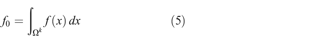
This paper define that the spatial domain of the input factor in the model recognition parameter is k-dimensional unit volume $Ω^{k}$ .

Ω^{k} = {x | 0 \leq x_{i} \leq 1, i = 1, 2, . . ., k}

(1)

Where, $Ω^{k}$ is the unit body, $x_{i}$ is the parameter, $k$ is the dimension.

According to the Taylor expansion, any function $f (x)$ can be expressed as the sum of sub-items.

\begin{matrix} f (x_{1}, x_{2}, . . ., x_{k}) = & f_{0} + \sum_{i = 1}^{k} f_{i} (x_{i}) + \sum_{1 \leq i < j \leq k} f_{ij} (x_{i}, x_{j}) \\ + \cdot \cdot \cdot f_{1, 2, . . ., k} (x_{1}, x_{2}, \dots, x_{k}) \end{matrix}

(2)

$2^{k}$ is the total number of decomposition term in equation (2). Sobol and Kucherenko proposed a decomposition method using multi-function integration.³⁹ The algorithm is characterized by:

① $f_{0}$ is a constant. The integration of each sub-item for any factor in equation (2) is 0, which can be expressed as

\int_{0}^{1} f_{i_{1}},_{i_{2}}, . . .,_{i_{s}} (x_{i_{1}}, x_{i_{2}}, . . ., x_{i_{s}}) d {x_{i}}_{j} = 0

(3)

② The sub-items are orthogonal. The condition for the existence of the equation (4) is that $(i_{1}, i_{2}, \cdot \cdot \cdot, i_{s}) \neq (j_{1}, j_{2}, \cdot \cdot \cdot, j_{l})$ exists.

\int_{Ω^{k}} {f_{i_{1}, i_{2}, \cdot \cdot \cdot i_{s}} \cdot f}_{j_{1}, j_{2}, . . ., j_{s}} dx = 0

(4)

The equation (3) has a unique decomposition form, and each sub-item can be obtained through multiple integration.

f_{0} = \int_{Ω^{k}} f (x) dx

(5)

f_{i} (x_{i}) = - f_{0} + \int_{0}^{1} \cdot \cdot \cdot \int_{0}^{1} f (x) d x_{- i}

(6)

f_{ij} (x_{i}, x_{j}) = - f_{0} - f_{i} (x_{i}) - f_{j} (x_{j}) + \int_{0}^{1} \cdot \cdot \cdot \int_{0}^{1} f (x) d x_{- (ij)}

(7)

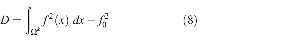
In equations (6) and (7), there exist $1 \leq i < j \leq k$ . Where, $x_{- i}$ represents the input factors other than $x_{i}$ , $x_{- (ij)}$ represents the input factors other than $x_{i}$ and $x_{j}$ .

The total variance of the proposed model is calculated as:

D = \int_{Ω^{k}} f^{2} (x) dx - f_{0}^{2}

(8)

The variance of the sub-terms of each order in equation (8) is the partial variance of each order, and its s-order partial variance can be expressed as

D_{i_{1}, i_{2}, \cdot \cdot \cdot i_{s}} = \int_{0}^{1} \cdot \cdot \cdot \int_{0}^{1} f_{i_{1}, i_{2}, \cdot \cdot \cdot, i_{s}}^{2} (x_{i_{1}}, x_{i_{2}}, \cdot \cdot \cdot, x_{i_{s}}) d x_{i_{1}} d x_{i_{2}} \cdot \cdot \cdot d x_{i_{s}}

(9)

From equations (2) and (9), the relationship between the total variance and the partial variance of each order can be expressed as

D = \sum_{i = 1}^{k} D_{i} + \sum_{1 \leq i < j \leq j} D_{ij} + \cdot \cdot \cdot D_{1, 2, \cdot \cdot \cdot k}

(10)

The sensitivity coefficient $S_{i_{1}, i_{2}, \cdot \cdot \cdot, i_{s}}$ is defined as the ratio of the deviation variance of each order $D_{i_{1}, i_{2}, \cdot \cdot \cdot i_{s}}$ over the total variance $D$ .

S_{i_{1}, i_{2}, \cdot \cdot \cdot, i_{s}} = \frac{D_{i_{1}, i_{2}, \cdot \cdot \cdot i_{s}}}{D}

(11)

Where, is the first-order sensitivity coefficient of factor $x$ ; $S_{ij} (i \neq j)$ is the second-order sensitivity coefficient; $S_{1, 2, \cdot \cdot \cdot, k}$ is the k-order sensitivity.

When many factors are considered to solve the sensitivity model, traditional Sobol’ solution approach is very computationally intensive and unstable.^40–42 In addition, due to various factors and their obvious coupling effects, the reliability problem of the actual engineering equipment structure is more complicated.

To address these challenges, optimal polynomial response surface functions between structural responses and model parameters are constructed by fitting samples based on the optimal error reduction ratio. Sensitivity values can then be obtained by direct integration.

This method has high matching accuracy, is easy to integrate directly, can effectively avoid a large number of sample calculations, and provides the possibility to analyze the coupling effect between multiple influencing factors.

The optimal polynomial response surface function can be combined by the complete polynomial of the parameter, expressed as

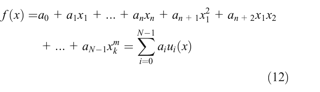
\begin{matrix} f (x) = & a_{0} + a_{1} x_{1} + . . . + a_{n} x_{n} + a_{n + 1} x_{1}^{2} + a_{n + 2} x_{1} x_{2} \\ + . . . + a_{N - 1} x_{k}^{m} = \sum_{i = 0}^{N - 1} a_{i} u_{i} (x) \end{matrix}

(12)

Where, $u_{i} (x)$ is the complete polynomial of variable $x = (x_{1}, x_{2}, . . . x_{n})$ ; $a_{i}$ is the undetermined coefficient; $N$ is the total number of polynomial terms, defined as

N = \frac{(n + m)!}{n! \cdot m!}

(13)

Equation (12) can be transformed into an orthogonal form, to determine the polynomial model coefficients, expressed as

f (k) = \sum_{i = 0}^{N - 1} h_{i} p_{i} (k)

(14)

Where, $f (k)$ is the target response value for the kth sampling, $k = 1, 2, . . ., L$ ; $p_{i} (k)$ is the orthogonal term under the kth sampling, which can be obtained by orthogonal transformation in equation (14); $h_{i}$ is the coefficient of the orthogonal term.

According to the orthogonality of each item in equation (14), it can be deduced into

\frac{1}{L} \sum_{k = 1}^{L} p_{i} (k) p_{j} (k) = 0

(15)

By using the Gram-Schmidt orthogonalization process,⁴³ $p_{i} (k)$ can be further expressed as

p_{i} (k) = u_{i} (k) - \sum_{j = 0}^{i - 1} α_{ij} p_{j} (k)

(16)

$u_{i} (k)$ is the k-th sampling polynomial.⁴⁴

And the coefficient $α_{ij}$ can be expressed as

α_{ij} = \frac{\sum_{k = 1}^{L} u_{i} (k) p_{j} (k)}{\sum_{k = 1}^{L} p_{j}^{2} (k)}

(17)

Define the error function Mean Square Error $(MSE)$ as⁴⁵

MSE = \frac{1}{L} \sum_{k = 1}^{L} (f (x) - \sum_{i = 0}^{N - 1} {h_{i} p_{i} (k))}^{2}

(18)

Set the derivative of $h_{i}$ in equation (18) equal to 0.⁴⁶ Then the coefficient of the orthogonal term $h_{i}$ can be expressed as⁴⁷

h_{i} = \frac{\sum_{k = 1}^{L} f (k) p_{i} (k)}{\sum_{k = 1}^{L} p_{i}^{2} (k)}

(19)

Equation (19) is substituted into equation (18) based on the orthogonality of $p_{i} (k)$ terms, and $h_{0}$ is always constant⁴⁸, then the error function MSE can be expressed as

MSE = \frac{1}{L} \sum_{d = 1}^{L} {(f (k))}^{2} - {(\frac{1}{L} \sum_{d = 1}^{L} f (k))}^{2} - \sum_{i = 1}^{N - 1} h_{i}^{2} (\frac{1}{L} \sum_{d = 1}^{L} p_{i}^{2} (k))

(20)

And the maximum value of MSE can be expressed as

MS E_{\max} = \frac{1}{L} \sum_{d = 1}^{L} {(f (k))}^{2} - {(\frac{1}{L} \sum_{d = 1}^{L} f (k))}^{2}

(21)

The contribution $C_{MSE}$ of the orthogonal term $p_{i} (k)$ to the reduction of MSE can be expressed as

C_{MSE} = \frac{1}{L} \sum_{k = 1}^{L} h_{i}^{2} p_{i}^{2} (k)

(22)

Then, in order to quantify the contribution of each orthogonal term to the reduction of the error function MSE, the error reduction ratio $ER R_{i}$ was expressed as⁴⁹

ER R_{i} = \frac{100 \cdot \sum_{d = 1}^{L} h_{i}^{2} p_{i}^{2} (k)}{\sum_{d = 1}^{L} {(f (k))}^{2} - \frac{1}{L} {(\sum_{d = 1}^{L} f (k))}^{2}}

(23)

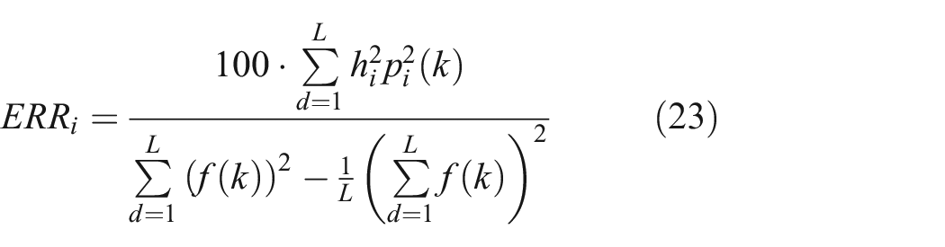
The contribution rate of the remaining items is solved by orthogonal transformation until the maximum $ER R_{i}$ of the remaining functional items is less than the set threshold. Further, the coefficient of reserved term in equation (8) can be obtained by the inverse orthogonal transformation, expressed as

a_{i} = \sum_{j = 1}^{N - 1} h_{j} q_{j}

(24)

q_{j} = - \sum_{r = i}^{j - 1} α_{jr} q_{r}

(25)

From this model, the coefficients of the polynomial optimal model and the target response function relative to the design parameters can be determined. The sensitivity of each parameter can be calculated directly by integral.

As shown in Figure 1, the limit function for structural reliability evaluation is established, and to identify the reliability influencing factors are included in the function. After that, the response surface function should be constructed, and the initial design points of which are defined. The least square approach is used to calculate the coefficients of response surface function, and based on which to solve the reliability index. After the solving process, the next generation design points should be constructed, and to generate all the design points, contain the experimental design points. Then the corrected coefficients of response surface function can be calculated, and the reliability index is solved again. Further, the response surface function can be solved by using the convergence judgment and loop calculation.

Figure 1.

Flow chart for solving response surface function.

Case study

Impact factors of structural reliability based on the revised sensitivity model

The sensitivity analysis approach based on revised sensitivity model can be proposed by combining multiple analysis steps, the flow chart of which is shown in Figure 2.

Figure 2.

Flow chart of the revised sensitivity model.

First of all, according to the working conditions of the equipment, the influence factors of the structure, the conventional value range of the influence factors, the number of sample points and variable space are studied. And the specific experimental scheme of various influencing factors can be made.

Then through the multi-body dynamics analysis, the load value corresponding to experimental group is calculated. And the load value of multi-body dynamics analysis is imported into the structural statics analysis step to accomplish the static analysis. Also the rationality of the experimental scheme is evaluated by the method of range verification. When the evaluation meets the requirements, the sensitivity value of each structural reliability factor are calculated, through the revised sensitivity model based on the response surface function. Then, the degree of influence of factors on reliability indexes and their coupling effects can be expressed quantitatively.

Experimental scheme

In order to verify the evaluation accuracy of the revised sensitivity model, a typical harvester structure is chosen to carry out the case study. In the context of considering the working environment for typical harvester structure, the controllable factors mainly include⁵⁰: forward speed $z_{1}$ , reel speed $z_{2}$ , stubble height $z_{3}$ , granary load $z_{4}$ , and threshing drum speed $z_{5}$ . The controllable influencing factors above are chosen as the experimental variables, and the maximum equivalent stress of the harvester structure is chosen as the evaluating indicator.

The common value of influencing factors for harvester structure as shown in Table 1 are obtained, according to the existing experimental research data. Relying on the concept of orthogonal experimental design.⁵¹

Table 1.

The design scheme of experimental factors.

Forward speed/( $m \cdot s^{- 1}$ )	Reel rotation speed/( $r \cdot min^{- 1}$ )	Stubble height/ $cm$	Granary load/ $t$	Drum rotation speed/( $r \cdot min^{- 1}$ )
0.25	133.6	10	2.06	280
0.45	116.8	15	1.74	410
0.66	100	20	1.42	540
1.28	83.4	25	1.1	670
1.48	66.7	30	0.78	800
1.69	50.1	35	0.46	980
2.31	33.3	40	0.14	1110

This is an experiment with five factors and seven levels. If all experiments have been conducted, 5⁷ = 78125 experimental combinations should be conducted. Therefore, the feasibility of comprehensive testing in practical applications is not high. At this point, orthogonal experiments are needed to determine the experimental combination. For tests with five factors and seven levels, there is an L49 (5⁷) orthogonal table that meets the conditions. Based on this, a testing plan was designed, which only requires 49 test combinations to obtain inspection indicators for operating parameters. Rules for interaction and influence. Combine the above working conditions with orthogonal experiments to obtain the L49 (5⁷) orthogonal experimental combination shown in Table 2

Table 2.

L₄₉ (5⁷) orthogonal test combinations.

Forward speed/( $m \cdot s^{- 1}$ )	Reel rotation speed/( $r \cdot min^{- 1}$ )	Stubble height/ $cm$	Granary load/ $t$	Drum rotation speed/( $r \cdot min^{- 1}$ )
0.25	133.60	10	2.06	280
0.25	116.80	20	1.10	800
0.25	100.00	30	0.14	410
0.25	83.40	40	1.42	980
0.25	66.70	15	0.46	540
0.25	50.10	25	1.74	1110
0.25	33.30	35	0.78	670
0.45	133.60	40	0.46	800
0.45	116.80	15	1.74	410
0.45	100.00	25	0.78	980
0.45	83.40	35	2.06	540
0.45	66.70	10	1.10	1110
0.45	50.10	20	0.14	670
0.45	33.30	30	1.42	280
0.66	133.60	35	1.10	410
0.66	116.80	10	0.14	980
0.66	100.00	20	1.42	540
0.66	83.40	30	0.46	1110
0.66	66.70	40	1.74	670
0.66	50.10	15	0.78	280
0.66	33.30	25	2.06	800
1.28	133.60	30	1.74	980
1.28	116.80	40	0.78	540
1.28	100.00	15	2.06	1110
1.28	83.40	25	1.10	670
1.28	66.70	35	0.14	280
1.28	50.10	10	1.42	800
1.28	33.30	20	0.46	410
1.48	133.60	25	0.14	540
1.48	116.80	35	1.42	1110
1.48	100.00	10	0.46	670
1.48	83.40	20	1.74	280
1.48	66.70	30	0.78	800
1.48	50.10	40	2.06	410
1.48	33.30	15	1.10	980
1.69	133.60	20	0.78	1110
1.69	116.80	30	2.06	670
1.69	100.00	40	1.10	280
1.69	83.40	15	0.14	800
1.69	66.70	25	1.42	410
1.69	50.10	35	0.46	980
1.69	33.30	10	1.74	540
2.31	133.60	15	1.42	670
2.31	116.80	25	0.46	280
2.31	100.00	35	1.74	800
2.31	83.40	10	0.78	410
2.31	66.70	20	2.06	980
2.31	50.10	30	1.10	540
2.31	33.30	40	0.14	1110

Multibody dynamics analysis

The software ADAMS is used to perform the multibody dynamics simulation of the harvester. The input conditions and boundary conditions imposed on structure are shown in Figure 3. The load is mainly concentrated on the connected position between the reel and the header, the header auger and the header, the cutting knife and header.⁵²

Figure 3.

Structural components and the loading conditions.

The boundary conditions are shown in Table 3. Also the driving function as shown in Table 4 are applied on the various pairs, in the software ADAMS. The obtained load spectrum at the reel, cutter, and auger are shown in Figure 4. Due to different working conditions, the three load values of the header structure show a fluctuating trend, among which the auger rotates the fastest, and its load value amplitude is the most obvious.

Table 3.

Boundary conditions.

Constraint object	Constraint type
Reel – Bearing	Rotating pair
Car body – Earth	Sliding pair
Header – Car body	Fixed pair
Wheel – Axle	Rotating pair
Drum – Header	Rotating pair

Table 4.

Driving function program of case structure.

Function type	Function expression	Meaning
Whole machine moving function	0.25*time	The forward speed is 0.25 m/s
Reel rotation function	Step (time,0,0,2,801.6d)	The reel rotation speed is 133.6 r/min
Drum rotation function	Step (time,0,0,2,1680d)	The drum rotation speed is 280 r/min

Figure 4.

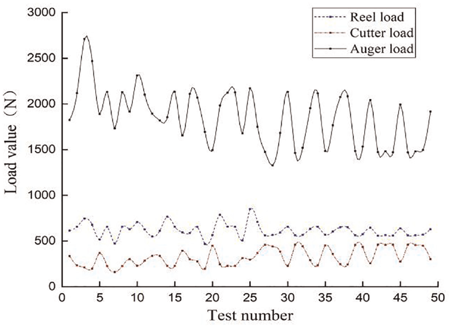
Load spectrum extracted from dynamic simulation.

Structural statics analysis

The 3D model is imported into the ANSYS software, and the loads at the reel, cutter, auger obtained from the dynamic analysis are set as the input parameters. Also the constraints are added at the feeding port. As shown in Figure 3, B is the load at the cutter, C and D are the load at the reel, E and F are the load at the auger, and fixed constraint is added at the feed port A. After the pre-processing is completed, 49 groups of data under the conditions of different matching influencing factors are input into the simulation process. Then the statics analysis cloud diagram under typical working conditions can be obtained, as shown in Figure 5. 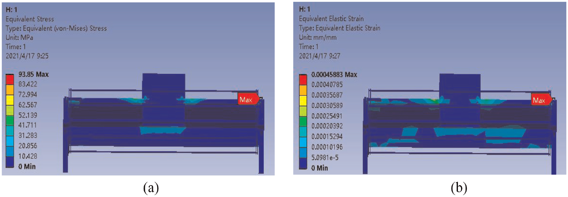Among them, the test plan corresponding to working condition 1 is: the speed of the threshing drum is 280 $r / min$ , the speed of the reel is 133.6 $r / min$ , the forward speed is 0.25 $m / s$ , the stubble height is 10 $cm$ , and the granary load is 2.06 $t$ .

Figure 5.

Statics analysis results under working condition 1: (a) equivalent stress and (b) equivalent strain.

The simulation results of 49 sets are shown in Figure 6. As shown in Figure 6. The average value of the test results are shown in Figure 6. The average prediction accuracy of the simulation results is 93.6%.

Figure 6.

Statics simulation and test results.

Range verification

The stress solution result for the influence factor under j-th column and $β$ -th level is $K_{β j}$ . $\bar{K_{β j}}$ is the average stress value of $K_{β j}$ , and $R_{j}$ is the range of the influence factor under j-th column, that is the difference between maximum value and minimum value of the j-th column factor index under each level.

R_{j} = max {{\bar{K}}_{1 j}, {\bar{K}}_{2 j}, . . ., {\bar{K}}_{β j}} - min {{\bar{K}}_{1 j}, {\bar{K}}_{2 j}, . . ., {\bar{K}}_{β j}}

(26)

$R_{j}$ is the maximum change of the test index when the level of the j-th column factor changes. The larger the $R_{j}$ , the more significant impact of the change of the influencing factor value on the test index is.

The range analysis model is used to analyze the data in the Figure 6, and the range analysis results as shown in Table 5 can be obtained. As shown in Table 5, the descending order of sensitivity degree for five influencing factors are: threshing drum speed, reel speed, forward speed, stubble height, and granary load. When the reliability is the control objective, the optimum threshing drum speed E should be the seventh level; the optimum reel speed B should be the second level; the optimum forward speed A should be the third level; the optimum stubble height C should be the seventh level; the optimum granary load D should take the first level. So the level combination of influencing factors is $A_{3} B_{2} C_{7} D_{1} E_{7}$ . It can be judged that the accuracy of simulation data under combination level is 96.37%, which guaranteed the rationality of the coupling factor experimental design.

Table 5.

Range analysis results of various influencing factors.

Factor	Forward speed	Reel rotation speed	Stubble height	Granary load	Drum speed
$K_{1 j}$	127.65	128.04	119.87	129.42	109.27
$K_{2 j}$	128.67	130.96	121.46	126.15	122.45
$K_{3 j}$	128.83	125.14	132.12	116.69	130.94
$K_{4 j}$	114.26	120.65	120.61	129.39	116.13
$K_{5 j}$	123.64	122.64	128.77	119.87	128.53
$K_{6 j}$	124.38	124.85	132.79	126.18	118.87
$K_{7 j}$	116.30	111.43	134.38	115.99	137.52
$R_{j}$	14.57	19.53	14.51	13.43	28.25
Ranking	3	2	4	5	1

Also nine groups of random prediction results shown in Figure 7 can be obtained, according to the range analysis results of various influencing factors, in which (a) is the simulated prediction value by the range analysis and (b) is the error rate. As shown in Figure 7, the stress corresponding to test number 17 is the largest, and its value is 154.79 MPa; the stress corresponding to test number 46 is the smallest, and its value is 84.15 MPa. The maximum error rate is 13.5%, which occurs in group 19. And the minimum error rate occurs in group 3, its value is 0.3%.

Figure 7.

The prediction results of range analysis.

Based on the above multi factor experimental analysis, the response surface function error contour map between the two structural strength influencing parameters of the harvester was obtained. It is obvious that there is a coupling relationship between the structural strength and parameters of the harvester. The relative error between the reel speed and the drum speed is the largest, as shown in Figure 8(g), while the relative deviation between the stubble height and the grain bin load is the smallest, as shown in Figure 8(h).

Figure 8.

Response surface function error fitting contour diagram: (a) error between F₁ and F₂, (b) error between F₁ and F₃, (c) error between F₁ and F₄, (d) error between F₁ and F₅, (e) error between F₂ and F₃, (f) error between F₂ and F₄ (g), error between F₂ and F₅, (h) error between F₃ and F₄, (i) error between F₃ and F₅, and (j) error between F₄ and F_5.

Sensitivity analysis

Local sensitivity analysis

The sensitivity analysis model mentioned above is used to calculate the sensitivity value of different influencing factors for the case structure. Then the results as shown in Table 6 can be obtained after the data summarizing.

Table 6.

The sensitivity for influencing factor of different level.

Influencing factor		Forward speed/ $m \cdot s^{- 1}$	Reel rotation speed/ $r \cdot min^{- 1}$	Stubble height/ $cm$	Granary load/ $t$	Drum rotation speed/ $r \cdot min^{- 1}$
Level	1	0.161	0.114	0.005	0.004	0.431
	2	0.147	0.123	0.005	0.003	0.471
	3	0.114	0.139	0.006	0.003	0.502
	4	0.094	0.152	0.006	0.002	0.520
	5	0.087	0.176	0.006	0.001	0.560
	6	0.075	0.196	0.006	0.001	0.614
	7	0.065	0.216	0.006	0.003	0.637

As shown in Figure 9, the sensitivity value of the drum rotation speed and the reel rotation speed shows an increasing trend with the change of level for single influencing factor, while the sensitivity value of forward speed shows a decreasing trend with the change of level for single influencing factor. Meanwhile, the sensitivity of granary load and stubble height are basically unchanged.

Figure 9.

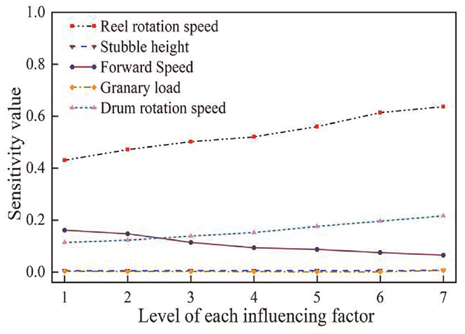
Sensitivity for single influencing factor.

The results can be obtained after the data summarizing, to quantitatively evaluate the sensitivity distribution interval of each influencing factor, as shown in Figure 10. As shown in Figure 10, the sensitivity value range of the drum rotation speed is the largest, and that of stubble height is the smallest.

Figure 10.

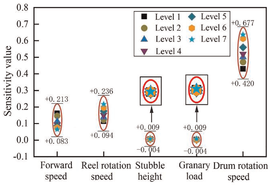
Sensitivity distribution range for single factor.

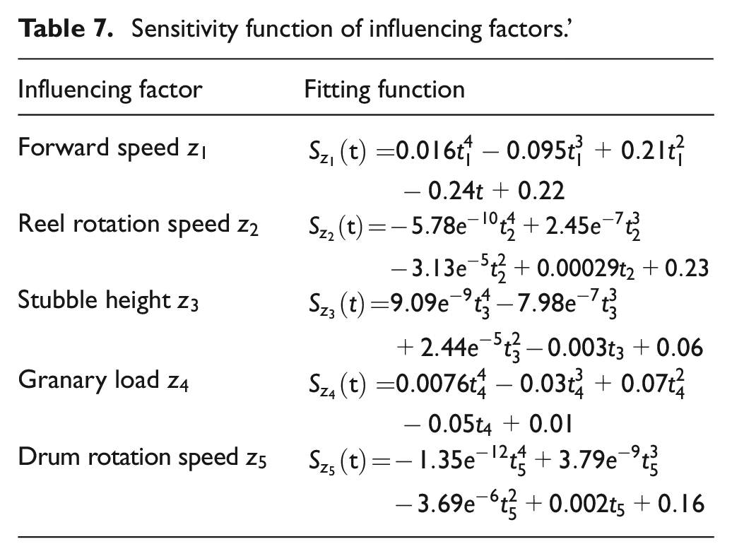
According to the results obtained in Figure 10, by fitting the sensitivity state distribution equation with Matlab, the sensitivity relationship functions of the five influencing factors shown in Table 7 can be obtained. Then the line diagram of sensitivity fitting function for the influencing factors can be obtained, as shown in Figure 11.

Table 7.

Sensitivity function of influencing factors.

Influencing factor	Fitting function
Forward speed $z_{1}$	$S_{z_{1}} (t) = 0.016 t_{1}^{4} - 0.095 t_{1}^{3} + 0.21 t_{1}^{2} - 0.24 t + 0.22$
Reel rotation speed $z_{2}$	$S_{z_{2}} (t) = - 5.78 e^{- 10} t_{2}^{4} + 2.45 e^{- 7} t_{2}^{3} - 3.13 e^{- 5} t_{2}^{2} + 0.00029 t_{2} + 0.23$
Stubble height $z_{3}$	$S_{z_{3}} (t) = 9.09 e^{- 9} t_{3}^{4} - 7.98 e^{- 7} t_{3}^{3} + 2.44 e^{- 5} t_{3}^{2} - 0.003 t_{3} + 0.06$
Granary load $z_{4}$	$S_{z_{4}} (t) = 0.0076 t_{4}^{4} - 0.03 t_{4}^{3} + 0.07 t_{4}^{2} - 0.05 t_{4} + 0.01$
Drum rotation speed $z_{5}$	$S_{z_{5}} (t) = - 1.35 e^{- 12} t_{5}^{4} + 3.79 e^{- 9} t_{5}^{3} - 3.69 e^{- 6} t_{5}^{2} + 0.002 t_{5} + 0.16$

Figure 11.

Sensitivity fitting line for each influencing factor.

Global sensitivity analysis for the influencing factors

The local sensitivity analysis is usually used to judge the influence of single factor.⁵³ So the global sensitivity analysis and the multiple-order sensitivity result are needed, to effectively confirm the coupling degree between influencing factors. The first-order sensitivity coefficient and the global sensitivity coefficient of the five influencing factors as shown in Table 8 are obtained, based on the revised sensitivity analysis model.

Table 8.

Global sensitivity value of influencing factors.

	Influence factor	Global sensitivity value
L1	Forward speed	0.149
L2	Reel rotation speed	0.368
L3	Stubble height	0.114
L4	Granary load	0.026
L5	Drum rotation speed	0.379

Then the specific influence degree of different factors can be effectively identified. Further, the distribution of sensitivity value for different influencing factors can be obtained as shown in Figure 12.

Figure 12.

Global sensitivity values of influencing factors.

As shown in Figure 12, the drum rotation speed and the reel rotation speed accounted for the largest proportion of sensitivity, the granary load and stubble height accounted for the smallest proportion. The sensitivity value of threshing drum speed is the largest, which further demonstrates that drum speed plays a leading role for the influence on case structure reliability. And the influence degree of the puller speed and the forward speed is different, which is mainly caused by the speed ratio of the puller speed and the forward speed. The load of the granary and the height of the stubble have little effect on the reliability of case structure during the harvester operation process.

The sensitivity prediction accuracy results shown in Table 9 are obtained by summarizing the simulation and test results. As shown in Table 9, the average value of sensitivity prediction accuracy of the case study is 97.36%.

Table 9.

The sensitivity prediction accuracy of factors.

Influencing factor	Prediction accuracy
Forward speed	97.23%
Reel Rotation speed	95.36%
Stubble height	97.52%
Granary load	98.24%
Drum rotation speed	98.45%

Considering the different factors affecting harvester operation under the analysis of global sensitivity, the optimal operation parameter range as shown in Figure 12 can be obtained, according to the results of global sensitivity distribution and equation (27).

ρ_{j} = \pm \frac{{[(1 - S_{j}) (1 - \frac{R_{j}}{\sum_{j = 1}^{5} R_{j}})]}^{\frac{1}{λ}}}{β^{\frac{2}{λ}}} \times 100 %

(27)

$ρ$ is the best operation parameter range of influencing factors; $S_{j}$ is the sensitivity value of influencing factors; $β$ is the number of influencing factors; $R_{j}$ is the maximum change of the test index when the level of the j-th column factor changes; $λ$ is the order number.

Figure 13 shows the best operation parameter ranges for different condition factors. As shown in Figure 13, the best operation parameter range of forward speed is between ±2.85% of K_4f; reel rotation speed is between ±1.98% of K_7r; stubble height is between ±2.97% of K_1s; granary load is between ±3.32% of K_7g; drum rotation speed is between ±1.71% of K_1d.

Figure 13.

The optimal operating parameters interval of case structure under first-order sensitivity revision.

Also the coupling relationship between different factors should also be considered, after analyzing the affection degree of single influencing factor. In order to further study the detailed sensitivity index, it is necessary to calculate the second order sensitivity value. The results shown in Table 10 are solved. $S_{ij}$ denotes the coupling of load $L_{i}$ and $L_{j}$ $(i \neq j)$ .

Table 10.

The second-order sensitivity of two-factor coupling.

Coupling factor	Second-order sensitivity value
L1 & L2 → S12	−0.021
L1 & L3 → S13	−0.016
L1 & L4 → S14	−0.016
L1 & L5 → S15	−0.006
L2 & L3 → S23	0.033
L2 & L4 → S24	0.009
L2 & L5 → S25	0.014
L3 & L4 → S34	−0.002
L3 & L5 → S35	0.007
L4 & L5 → S45	0.006

And the sensitivity index distribution of the parameters can be obtained, as shown in Figure 14. The coupling degree between the reel speed and the stubble height is the most prominent, and the coupling degree between the stubble height and the threshing drum speed is the least prominent. At the same time, the analysis results show that the interaction between the influencing factors produces the total order sensitivity of the analysis.

Figure 14.

Sensitivity distribution of coupling factors.

Considering the different degrees of factors affecting harvester operation under the analysis of second-order sensitivity, the optimal operation parameter range as shown in Figure 15 can be obtained, according to the results of global sensitivity distribution and equation (27). Figure 15 illustrates the best range of operation parameters for different condition factors. As shown in Figure 15, the best operation parameter range of forward speed is between ±1.77% of K_4f; reel rotation speed is between ±1.70% of K_7r; stubble height is between ±1.78% of K_1s; granary load is between ±1.81% of K_7g; drum rotation speed is between ±1.63% of K_1d.

Figure 15.

The optimal operating parameters interval of case structure under second-order sensitivity revision.

The distribution of optimal operating parameters interval under five order sensitivity revision can be achieved, as shown in Figure 16. With the increase of the order, the optimal value range is gradually reduced. With the increase of the order of the solution, the range of the optimal operation parameters is gradually refined. From the point of view of protecting the operation safety of the equipment structure, a more detailed range of operation parameters is beneficial.

Figure 16.

The distribution of optimal operating parameters interval under five order sensitivity revision.

Conclusion

This paper has developed a response surface modified sensitivity model for local and global sensitivity analysis of multiple influencing factors, by integrating the optimal polynomial response surface function with the Sobol’ algorithm. Through the direct integration of the revised sensitivity reliability model, the accurate multiple-order sensitivity index of mechanical structure can be obtained. Not only the change of single factor, but also the mutual coupling between the factors are studied.

The industrial case shows that the proposed revised approach has a high prediction accuracy of 97.36%. The results reveal that the coupling induction between the reel rotation speed (L2) and the stubble height (L3) is the highest, and the coupling induction between the stubble height (L3) and the drum rotation speed (L5) is the weakest. Based on this method, other industrial cases can be analyzed, to get the coupling induction of different working conditions.

The distribution of optimal operating parameters interval under five order sensitivity revision are achieved. With the increase of the order, the optimal value range is gradually reduced. The revised approach may provide a good mean for the choose of the best operation parameters of equipment.

Footnotes

Handling Editor: Chenhui Liang

Declaration of conflicting interests

The author(s) declared no potential conflicts of interest with respect to the research, authorship, and/or publication of this article.

Funding

The author(s) disclosed receipt of the following financial support for the research, authorship, and/or publication of this article: This work was supported by National Natural Science Foundation of China (51805447), Natural Science Foundation of Jiangsu Province (BK20190911), Agricultural Science and Technology Independent Innovation Fund of Jiangsu Province (CX(20)3060), Natural Science Foundation of the Jiangsu Higher Education (22KJB460010).

References

Zhu

Jia

Lin

, et al. Structural health assessment method combining stress concentration factor and Bayesian theory. Chin J Mech Eng 2019; 55: 21–27.

Zhao

Jia

Bin

, et al. Multiple-order graphical deep extreme learning machine for unsupervised fault diagnosis of rolling bearing. IEEE Trans Instrum Meas 2021; 70: 3506012.

Zhang

Qin

, et al. VoI-informed decision-making for SHM system arrangement. Struct Health Monit Int J 2022; 21: 37–58.

Yan

Gao

. Hilbert-Huang transform-based vibration signal analysis for machine health monitoring. IEEE Trans Instrum Meas 2006; 55: 2320–2329.

Zhou

, et al. Multiscale dynamic fusion global sparse network for gearbox fault diagnosis. IEEE Trans Instrum Meas 2021; 70: 3516111.

Wang

Yang

, et al. Structural design optimization based on hybrid time-variant reliability measure under non-probabilistic convex uncertainties. Appl Math Model 2019; 69: 330–354.

Gazi

Alhan

. Reliability of elastomeric-isolated buildings under historical earthquakes with/without forward-directivity effects. Eng Struct 2019; 195: 490–507.

Owerko

Winkelmann

Gorski

. Application of probabilistic tools to extend load test design of bridges prior to opening. Struct Infrastruct Eng 2020; 16: 931–948.

Zhang

Anderson

Bland

, et al. All-printed strain sensors: Building blocks of the aircraft structural health monitoring system. Sens Actuators A Phys 2017; 253: 165–172.

10.

Barranco-Cicilia

Lima

ECP

Sagrilo

LVS

. Reliability-based design criterion for TLP tendons. Appl Ocean Res 2008; 30: 54–61.

11.

Liu

Zhang

Mao

. Analysis of influencing factors in pre-evacuation time using interpretive structural modeling. Saf Sci 2020; 128: 104785.

12.

Pereira

Ahn

Han

, et al. Finding causal paths between safety management system factors and accident precursors. J Manag Eng 2020; 36: 04019049.

13.

Xiao

, et al. Maximum variation analysis based analytical target cascading for multidisciplinary robust design optimization under interval uncertainty. Adv Eng Inform 2019; 40: 81–92.

14.

Xiao

Garg

, et al. A new approach to solve uncertain multidisciplinary design optimization based on conditional value at Risk. IEEE Trans Autom Sci Eng 2021; 18: 356–368.

15.

Wang

, et al. Energy saving design optimization of CNC machine tool feed system: A data-model hybrid driven approach. IEEE Trans Autom Sci Eng 2022; 19: 3809–3820.

16.

Xiao

Gao

. Improved collaboration pursuing method for multidisciplinary robust design optimization. Struct Multidiscipl Optim 2019; 59: 1949–1968.

17.

Zhang

Song

Fei

, et al. Advanced multiple response surface method of sensitivity analysis for turbine blisk reliability with multi-physics coupling. Chin J Aeronaut 2016; 29: 962–971.

18.

Zhu

Keshtegar

Bagheri

, et al. Novel hybrid robust method for uncertain reliability analysis using finite conjugate map. Comput Methods Appl Mech Eng 2020; 371: 113309.

19.

Scozzese

Gioiella

Dall’Asta

, et al. Influence of viscous dampers ultimate capacity on the seismic reliability of building structures. Struct Saf 2021; 91: 102096.

20.

Haddadi

El Fellahi

, et al. Setting parameters influence on accuracy and stability of near-field scanning microwave microscopy platform. IEEE Trans Instrum Meas 2016; 65: 890–897.

21.

Dashliborun

Larachi

. CFD study and experimental validation of multiphase packed bed hydrodynamics in the context of rolling sea conditions. AIChE J 2019; 65: 385–397.

22.

Chung

Ihme

. Examination of diesel spray combustion in supercritical ambient fluid using large-eddy simulations. Int J Engine Res 2020; 21: 122–133.

23.

Caparco

Wang

Das

, et al. Tuning the morphology of protein-inorganic calcium-phosphate supraparticles via directed assembly. Langmuir 2020; 36: 15296–15308.

24.

Andreini

Bacci

Insinna

, et al. Modelling strategies for the prediction of hot streak generation in lean burn aeroengine combustors. Aerosp Sci Technol 2018; 79: 266–277.

25.

Sudret

. Global sensitivity analysis using polynomial chaos expansions. Reliab Eng Syst Saf 2008; 93: 964–979.

26.

Abbiati

Marelli

Tsokanas

, et al. A global sensitivity analysis framework for hybrid simulation. Mech Syst Signal Process 2021; 146: 106997.

27.

Sudret

Mai

. Computing derivative-based global sensitivity measures using polynomial chaos expansions. Reliab Eng Syst Saf 2015; 134: 241–250.

28.

Greco

Trentadue

. Structural reliability sensitivities under nonstationary random vibrations. Math Probl Eng 2013; 2013: 426361.

29.

Zhang

Zhou

, et al. Frequency reliability sensitivity for dynamic structural systems. Mech Based Des Struct Mach 2010; 38: 74–85.

30.

Dong

Sheng

Zhao

, et al. Robust optimization design method for structural reliability based on active-learning MPA-BP neural network. Int J Struct Integr 2023; 14: 248–266.

31.

Liu

Tong

, et al. Mixed uncertainty analysis for dynamic reliability of mechanical structures considering residual strength. Reliab Eng Syst Saf 2021; 209: 107472.

32.

Zhang

Liu

, et al. Reliability analysis of excavator boom considering mixed uncertain variables. Qual Reliab Eng 2021; 37: 1468–1483.

33.

Jiang

Liu

Wang

, et al. Interval dynamic reliability analysis of mechanical components under multistage load based on strength degradation. Qual Reliab Eng Int 2021; 37: 576–582.

34.

Jensen

Mayorga

Valdebenito

. Reliability sensitivity estimation of nonlinear structural systems under stochastic excitation: A simulation-based approach. Comput Methods Appl Mech Eng 2015; 289: 1–23.

35.

Zhu

Qiu

Chen

, et al. Approach for the structural reliability analysis by the modified sensitivity model based on response surface function - Kriging model. Heliyon 2022; 8: e10046.

36.

Nariman

. Aerodynamic stability parameters optimization and global sensitivity analysis for a cable stayed bridge. KSCE J Civil Eng 2017; 21: 1866–1881.

37.

Huang

Zhao

. Probabilistic flutter analysis of bridge considering aerodynamic and structural parameter uncertainties. J Wind Eng Ind Aerodynamics 2020; 201: 104168.

38.

Hamdia

Ghasemi

Zhuang

, et al. Sensitivity and uncertainty analysis for flexoelectric nanostructures. Comput Methods Appl Mech Eng 2018; 337: 95–109.

39.

Sobol

Kucherenko

. Derivative based global sensitivity measures. Proc Soc Behav Sci 2010; 2: 7745–7746.

40.

Azzini

Rosati

. Sobol' main effect index: an Innovative Algorithm (IA) using dynamic adaptive variances. Reliab Eng Syst Saf 2021; 213: 107647.

41.

Chen

Lin

Wang

, et al. Further results on orthogonal arrays for the estimation of global sensitivity indices based on alias matrix. Stat Methods Appl 2015; 24: 411–426.

42.

Carneiro

Antonio

. Sobol' indices as dimension reduction technique in evolutionary-based reliability assessment. Eng Comput 2020; 37: 368–398.

43.

Rivaz

Moghadam

Sadeghi

, et al. An approach of orthogonalization within the Gram–Schmidt algorithm. Comput Appl Math 2018; 37: 1250–1262.

44.

Chiachío

Saxena

, et al. Bayesian model selection and parameter estimation for fatigue damage progression models in composites. Int J Fatigue 2015; 70: 361–373.

45.

Yun

Feng

, et al. Two efficient AK-based global reliability sensitivity methods by elaborative combination of Bayes' theorem and the law of total expectation in the successive intervals without overlapping. IEEE Trans Reliab 2020; 69: 260–276.

46.

Garcia-Cabrejo

Valocchi

. Global sensitivity analysis for multivariate output using polynomial chaos expansion. Reliab Eng Syst Saf 2014; 126: 25–36.

47.

Wei

Wang

Tang

. Time-variant global reliability sensitivity analysis of structures with both input random variables and stochastic processes. Struct Multidiscipl Optim 2017; 55: 1883–1898.

48.

Wei

Liu

, et al. A probabilistic procedure for quantifying the relative importance of model inputs characterized by second-order probability models. Int J Approx Reason 2018; 98: 78–95.

49.

Qian

Massenzio

Brizard

, et al. Sensitivity analysis of complex engineering systems: Approaches study and their application to vehicle restraint system crash simulation. Reliab Eng Syst Saf 2019; 187: 110–118.

50.

Yin

Qin

Zhang

, et al. Compensation control strategy for the cutting frequency of the cutterbar of a combine harvester. Biosyst Eng 2021; 204: 235–246.

51.

Fang

Liski

. A new approach in constructing orthogonal and nearly orthogonal arrays. Metrika 2000; 50: 255–268.

52.

Guan

Tang

. Experiments on influencing factors of cutting force of rape stem. Trans Chin Soc Agric Eng 2009; 25: 141–144.

53.

van Keulen

Haftka

Kim

. Review of options for structural design sensitivity analysis. Part 1: Linear systems. Comput Methods Appl Mech Eng 2005; 194: 3213–3243.

Influence of coupling factors on structural reliability based on polynomial response surface optimization model

Abstract

Keywords

Introduction

Revised sensitivity model

Case study

Impact factors of structural reliability based on the revised sensitivity model

Experimental scheme

Multibody dynamics analysis

Structural statics analysis

Range verification

Sensitivity analysis

Local sensitivity analysis

Global sensitivity analysis for the influencing factors

Conclusion

Footnotes

Declaration of conflicting interests

Funding

References