Integration of multiple failure mechanisms in a life assessment method for centrifugal pump impellers

Abstract

Methods in predictive maintenance are frequently confronted with limited applicability to realistic scenarios. The available approaches are often used for a single design, requiring an entirely new analysis for a slightly different case. A solution for this issue could be using a physical model. However, physical models focus on one unique failure mechanism, while, in a practical application, several mechanisms are typically active at the same instant. This work proposes and demonstrates a new methodology that combines different failure mechanism into an integrated life prediction model. Failure Modes and Effects Analysis is used to identify the different failure mechanisms that occur in a component simultaneously. Physical and empirical models are then analyzed and modified to be implemented in a realistic case of a centrifugal pump impeller applied in a maritime environment. As erosion, cavitation, and corrosion are the main failure mechanisms of an impeller, the combination of them quantifies the degradation increment during different types of pump operation. The proposed methodology is compared with traditional failure rate models and an established cavitation model that uses an aging factor to cover other failure mechanisms. In conclusion, it is demonstrated that the proposed methodology is more sensitive and reliable in describing the degradation process for a wide range of operating conditions, since all the mechanisms are considered.

Introduction

Maintenance represents a significant fraction of the total operational costs of many assets. Therefore, methodologies are constantly being developed to decrease losses and achieve reliable and efficient operations. For example, Kimera and Nangolo ¹ proposed a stochastic optimization model to determine the maintenance interval that provides the optimal balance between costs and system performance for marine mechanical systems. Further, diagnostic strategies focus on fault detection, isolation, and identification. ² Complementary Ensemble Empirical Mode Decomposition and bispectrum imaging are examples of diagnostic techniques used to identify stages of cavitation in centrifugal pumps.^3,4 However, these techniques are not sufficient to predict the future behavior of the equipment, so a strategy to deal with this must be developed.

In predictive maintenance, the most advanced maintenance policy that attracts a lot of attention nowadays, also various tools and models are used to optimize maintenance intervals. The first approach considered here is the group of data-driven methods. These methodologies are based on historic failure data or sensor data, and typically focus on the failure of a component in a specific case or scenario. For example, some authors use vibration data and performance measurements to predict the remaining useful life (RUL) of the component.^5,6 The model on diesel engine fault prediction as proposed by Liu et al. ⁷ uses a neural network to predict the ship engine exhaust temperature and aims to detect differences between measured and predicted values. Mohammed ⁸ also presented a data-driven approach using multiple linear regression, where the data collected was based on both expert knowledge and pump failures. This approach seems to be feasible for use in a variety of applications, although this is not explicitly demonstrated in the paper. However, as in this approach the models fully depend on the specific data-set used, the complete analysis needs to be redone when the component application or environment is changed. Moreover, these methodologies are often applied when there is a lot of data available and no physical model describing the dominant failure mechanism.

In the second approach, the models use historical failure rates as the main factor for failure prediction. ⁹ For example, the failure rate models in the handbook NSWC-11 ¹⁰ are derived from sources or theories that have already been consolidated in the literature. Such models use the failure rate and some additional physical equations to describe the component failure behavior under different operating conditions, but can typically not distinguish between different failure mechanisms.

The third approach uses physical models to describe the components’ failure behavior. Physical models are accurate mathematical models in which a failure mechanism is quantitatively characterized using physical laws. ¹¹ These methods simulate the degradation of a component^12,13 with a mathematical model and usually address a unique failure mechanism. However, this may complicate the coverage of the total degradation (typically being a combination of different failure mechanisms) in a real application. An example of a single failure mechanism approach is the physical corrosion model for bioabsorbable metal stents presented by Grogan et al., ¹⁴ assuming that the corrosion is driven by magnesium diffusion alone. Other failure mechanisms are not considered, which limits the applicability of the approach. Sackett and Narasimhan ¹⁵ examined the current approaches in mathematical modeling of the degradation of polymers, and it is observed that most of the models examine only one of the failure mechanisms. Also the fretting motion prediction model for controllable pitch propellors (CPP), as proposed by Godjevac et al., ¹⁶ only considers the fretting failure mechanism, while for a CPP also fatigue and abrasive wear could lead to failure. The authors mentioned above suggest that combining models that account for different phenomena could be a way to overcome this gap. This reveals that existing methods have at least one of the three main limitations: (i) models only work for the specific situation they are derived for (data-driven); (ii) models cannot distinguish between individual failure mechanisms (failure rate models); (iii) models only consider one specific failure mechanism (physical models).

For the specific case of the centrifugal pump impeller, the focus of this work, different approaches can be found in the literature to describe the degradation and many of them use physical models. However, it is important to evaluate whether the so-called physical model is purely physical or is combined with a data-driven approach (a hybrid model). ¹⁷ The main failure mechanisms, leading to insufficient yield in the impeller, are cavitation causing fatigue damage, wear by erosion of particles in the fluid, and corrosion due to exposure to seawater or high-temperature fluids. ¹⁸ Physical corrosion models are not well established in the literature. ¹⁹ Thus, an empirical model is an alternative; such a model is generally developed based on data collected from the field or from experiments, ²⁰ but still includes the governing physical quantities (e.g. temperature).

Physical models that describe the cavitation phenomena can use different approaches. Some authors use computational fluid dynamics to analyze centrifugal pump performance under developed cavitating conditions. ²¹ However, this is a purely numerical model, and experimental validation is required. ²² In 2003, the Turbomachinery Society of Japan presented a guideline for predicting and evaluating the cavitation degradation in pumps. ²³ Such a physical methodology calculates the cavitation erosion rate at the maximum damage point. However, it was observed that the scatter in the measured rates is about twice the one in predicted rates. Therefore, Hattori and Kishimoto ²⁴ proposed a methodology that reduces this gap between measured and predicted rate. Further, cavitation is not the only mechanism addressed in this approach; some scaling factors are used to cover the other mechanisms, such as erosion and corrosion. However, such factors don’t cover all possible scenarios and therefore delimit the method’s application range.

Furthermore, many authors discuss erosion models to describe material loss during the operation.^25,26 Archard’s equation is often used to calculate the wear volume loss between metal contact surfaces. ²⁷ Moreover, Serrano et al. ²⁸ proposed a methodology to calculate the amount of worn material of an impeller using Archard and Hirst’s wear law. ²⁹ However, this technique covers only erosion degradation, and the impeller is also worn by cavitation and corrosion as discussed before.

It can be concluded that approaches that address multiple (potentially interacting) failure mechanisms are rather scarce in the literature. This holds for the specific case of the pump impeller, but also more generically. Besides that, it would be convenient to use a technique that applies a unique model to multiple scenarios. This work brings a solution for these issues; it focuses on an impeller of a centrifugal pump, but it can rather easily be extended to other applications.

In this work, the authors present a new methodology to combine models, that is, to accumulate degradation, covering the main failure mechanisms (FM) for the pump impeller. These mechanisms are identified through the Failure Modes and Effects Analysis (FMEA), and the associated prediction models are then integrated. The combination of the models delivers the total degradation increment at each instance; besides, it also reveals which of the failure mechanisms is dominant in a specific situation. Such insights can be used to optimize the system and extend the lifetime of the component.^30,31 Finally, the proposed methodology is compared with different approaches that are available in the literature, by simulating various scenario’s.

The original contribution of this work is firstly the structured review and numerical comparison of three different types of life prediction methods for centrifugal pump impellers. Secondly, the main scientific contribution is the integration of three separate (and existing) physical degradation models into a formulation that allows to consider them simultaneously. This requires adaptation of the three models to yield a common degradation parameter, and to use similar load parameters as input. This process is developed and demonstrated for a centrifugal pump case, but is generic in nature.

This paper is organized in the following way. Firstly, in section “Failure mechanism identification,” the process of identifying the relevant failure mechanisms is described. In section “Current models for impeller life time and reliability,” the current models in the literature are analyzed, and the issues or applicability of these approaches are investigated. In section “Integrated life prediction model,” the models are adjusted and the new methodology integrating the various failure mechanisms is proposed. In section “Comparison of different models,” the different models are compared based on practical applications. Finally, sections “Model development challenges” and “Conclusion” contain the results discussion and the conclusions of the work.

Failure mechanism identification

A key element in the development of the proposed life assessment model is the identification of the relevant failure mechanisms for the component under consideration. The usage of pumps is extensively observed in maritime, industrial, infrastructure, and military sectors. For the case study analyzed in this work, a pump used in ship fire fighting systems was selected. The specification of the pump is NISM 125-250/01 from Allweiler, see Figure 1. In this section the functional failure modes as well as the failure mechanisms for this system will be analyzed. With this starting point it is possible to recognize the failure mechanisms that together cover most of the degradation phenomena in the selected critical component of the pump. Based on this information, the proposed method, later denoted as physical combination model (PCM), can be developed.

Figure 1.

Centrifugal pump driven by an electric motor and closed impeller.

The process of the failure mechanism identification is presented schematically in Figure 2. It is based on the failure analysis method proposed by Peeters et al., ³³ combining Failure Modes, Effects and Criticality Analysis (FMECA) and Fault Tree Analysis (FTA) in a recursive manner. The first step of the methodology is making a fault tree for the systems level (i.e. the pump in this case). However, as a detailed analysis of the complete fault tree would be too extensive, only one intermediate event is selected for further analysis, while the others are neglected. For that, the most critical event is selected using the Risk Priority Numbers (RPN) in an FMECA analysis. This selection can be based on failure data (from a Computerized Maintenance Management System (CMMS) or expert experience, i.e. FMEA).^34,35 The same methodology for prioritizing parts of the fault tree is then applied at the functional and component level, ultimately leading to a list of relevant failure mechanisms (see bottom part of Figure 2). For the case analyzed, FMEA was used in each level, where experts selected the most critical branch of the fault tree. As a result, for the impeller of a centrifugal pump erosion, cavitation, and corrosion are determined to be the main failure mechanisms. Note that this assessment of the failure mechanisms is essential when developing physics-based life prediction models. The procedure from Peeters et al. ³³ assists in structuring this process, but it is still not trivial to execute. Specific domain and system knowledge is required to find the relevant failure modes and mechanisms.

Figure 2.

FTA and FMEA in a recursive technique for the centrifugal impeller.

Current models for impeller life time and reliability

The life prediction method proposed in this work combines models of various failure mechanisms. The models for these individual failure mechanisms are already available in the literature. However, some modifications are needed to solve some inconsistencies in these models, so these will be introduced and briefly discussed in this section. Firstly, the traditional failure rate model will be described, as that will be used as the benchmark for the proposed method.

Failure rate model

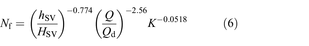
A commonly applied method to quantify the reliability of a pump is the failure rate model. This method uses the empirically determined base failure rate and some additional physical equations to describe the component failure behavior under different operating conditions. As this approach is already available in the literature, it will be used as a reference method in this work, to which other approaches will be benchmarked. The failure rate for the pump fluid driver, that is, the impeller, is calculated as follows ¹⁰ :

$${\lambda }_{\mathrm{FD}}={\lambda }_{\mathrm{FD},\mathrm{B}}{C}_{\mathrm{PF}}{C}_{\mathrm{PS}}{C}_{\mathrm{C}}{C}_{\mathrm{SF}}$$

(1)

In this equation, ${\lambda }_{\mathrm{FD}}$ is the failure rate for the fluid driver [failure/million operating hours], ${\lambda }_{\mathrm{FD},\mathrm{B}}$ is the base failure rate [failure/million operating hours], $C_{\mathrm{PF}}$ is the percent flow multiplying factor [−], $C_{\mathrm{PS}}$ is the operating speed multiplying factor [−], $C_{\mathrm{C}}$ is the contaminant multiplying factor [−], and $C_{\mathrm{SF}}$ is the service factor multiplying factor [−]. This equation quantifies the impeller failure rate by multiplying the base failure rate with four different influence factors. These factors are related to respectively the magnitude of the flow, the pump operating speed, the presence (and size) of contaminants in the fluid, and the service loads. In NSWC-11, ¹⁰ the base failure rate ( ${\lambda }_{\mathrm{FD},B}$ ) is reported to vary between 0.12 and 0.2 failures per million hours of operation for a centrifugal pump. However, in other literature sources much higher values are reported for this failure rate, for example, around 7.275 failures per million hours of operation. ³⁶ It is also noted that ${\lambda }_{\mathrm{FD},B}$ can vary vastly due to many factors, such as the installation.^5,37 This indicates the need for obtaining a value for the base failure rate typical for the application considered, as is advised for many other components in the handbook. Such a value can typically be provided by the manufacturer.

The detailed expressions for the multiplication factors will be discussed next. The expression for the percent flow multiplying factor is as follows^38–40:

$$\mathrm{For}0.1\le Q/Q_{\mathrm{r}}\le 1.0:$$

$$C_{\mathrm{PF}}=9.94-0.90\left(\frac{Q}{Q_{\mathrm{r}}}\right)-10{\left(\frac{Q}{Q_{\mathrm{r}}}\right)}^2+1.77{\left(\frac{Q}{Q_{\mathrm{r}}}\right)}^3$$

(2a)

$$\mathrm{For}1.0\le Q/Q_{\mathrm{r}}\le 1.1:$$

$$C_{\mathrm{PF}}=1.0$$

(2b)

$$\mathrm{For}1.1\le Q/Q_{\mathrm{r}}\le 1.7:$$

$$C_{\mathrm{PF}}=-30.6+36\left(\frac{Q}{Q_{\mathrm{r}}}\right)-4.5{\left(\frac{Q}{Q_{\mathrm{r}}}\right)}^2-2.2{\left(\frac{Q}{Q_{\mathrm{r}}}\right)}^3$$

(2c)

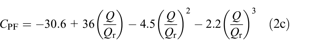
In these equations and also presented in Figure 3, $Q$ is the discharge at the operating point $[{\mathrm{m}}^3/\min ]$ and $Q_{\mathrm{r}}$ is the maximum pump specific flow $[{\mathrm{m}}^3/\min ]$ .

Figure 3.

Percent flow multiplying factor as a function of pump capacity.

The operating speed factor is determined with the following equation, Figure 4 ¹⁰ :

$$C_{\mathrm{PS}}=5{\left(\frac{V_{\mathrm{O}}}{V_{\mathrm{D}}}\right)}^{1.3}$$

(3)

Figure 4.

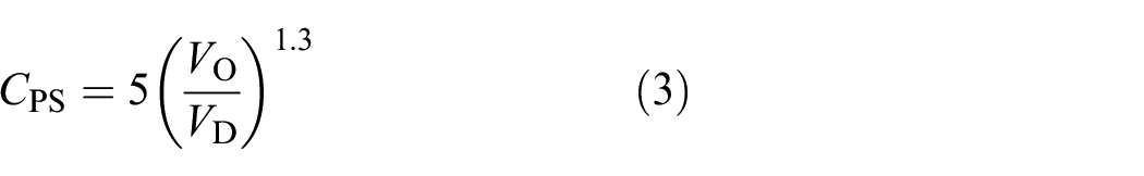
Pump operating speed multiplying factor.

where $V_O$ is the operating speed $[\mathrm{m}/\mathrm{s}]$ and $V_{\mathrm{D}}$ is the maximum allowable design speed $[\mathrm{m}/\mathrm{s}]$ .

And finally, the contaminant factor $C_{\mathrm{C}}$ , Figure 5, which considers the filter size, is given by:

$$C_{\mathrm{C}}=0.6+0.05F_{\mathrm{AC}}$$

(4)

Figure 5.

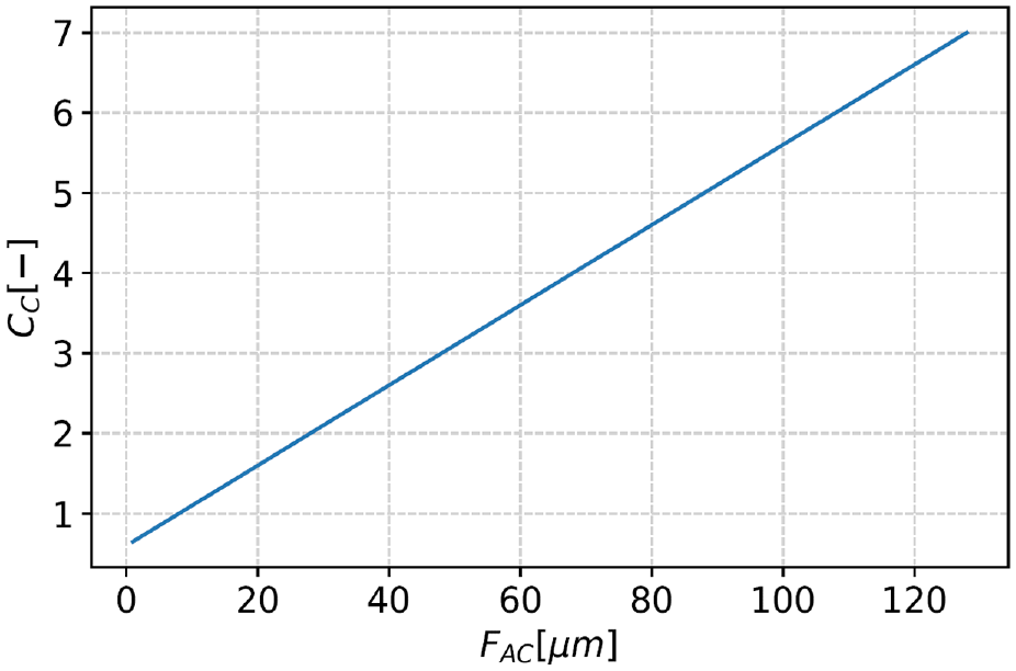
Particle size multiplying factor.

However, in a practical application the filter size does not determine the size of the contaminants in the fluid, but only the maximum size of the particles. In many applications, the particle size distribution, therefore, differs from the filter size. Besides that, the filter type also influences the particle size. ⁴¹ For this reason, it is proposed here to consider the actual value of particle size for the parameter $F_{\mathrm{AC}}$ $\left[\mu \mathrm{m}\right]$ and not the filter size.

To conclude, the above equations raised some issues, indicating the need to check and understand the background of available methods. With the proposed modifications, this model can be used and compared with other models that will be discussed in the following subsection. The model without these modifications is analyzed and discussed in previous work. ⁴²

Physical and empirical models

For the impeller, a number of physical and empirical models are available. As discussed before, none of the models covers all failure mechanisms, so a combination of them seems necessary. The physical models are based on equations with a physical meaning, while an empirical model is an expression fitted to a data-set collected from the field or experiments. Three specific models were selected and will be introduced here.

Cavitation model

Cavitation occurs when bubbles develop in the pumped fluid, which subsequently collapse and cause shock waves. These shocks lead to (fatigue and wear) damage in the impeller material. The model to calculate the cavitation wear rate at the maximum damage point $E{R}_p$ $[\mathrm{m}/\mathrm{s}]$ will be analyzed and discussed. Equation (5) is a non-dimensional equation that is used to predict the degradation increment by cavitation. ²⁴

$$\frac{E{R}_{\mathrm{p}}}{D_{\mathrm{e}}2\pi \omega }=4.57·{10}^{-12}{N}_{\mathrm{f}}{\left(\frac{\mathrm{HV}}{197}\right)}^{-1.13}{m}_1{m}_2{m}_3{m}_4$$

(5)

where $D_{\mathrm{e}}$ is the eye diameter of the impeller $\left[\mathrm{m}\right]$ , see Figure 6, $\omega$ is the rotational speed $\left[{\mathrm{s}}^{-1}\right]$ , $\mathrm{HV}$ is the Vickers hardness of the material $\left[\mathrm{HV}\right]$ , and $N_f$ is the flow factor [−], see equation (6). The factors $m_1$ , $m_2$ , $m_3$ , and $m_4$ represent the relative effects of temperature, aging, type of fluid, and influence of microstructure, respectively. These factors were introduced by Hattori and Kishimoto ²⁴ to predict the damage due to effects other than cavitation. The impeller dimensions that are needed as input for the physical models are indicated in Figure 6.

Figure 6.

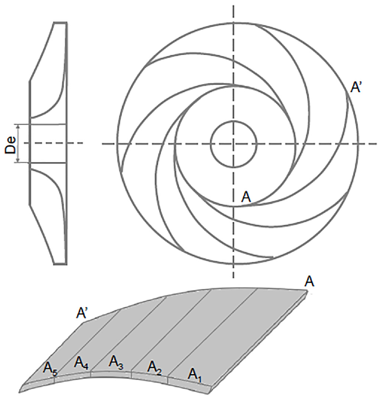
Impeller dimensions.

As the occurrence of cavitation in a pump fully depends on the flow conditions, the most important factor in equation (5) is the flow factor $N_f$ :

$$N_{\mathrm{f}}={\left(\frac{h_{\mathrm{SV}}}{H_{\mathrm{SV}}}\right)}^{-0.774}{\left(\frac{Q}{Q_{\mathrm{d}}}\right)}^{-2.56}{K}^{-0.0518}$$

(6)

where $h_{\mathrm{SV}}$ is the actual net positive suction head NPSH_a $\left[\mathrm{m}\right]$ , see equation (8), $H_{\mathrm{SV}}$ is the allowable net positive suction head NPSH_r $\left[\mathrm{m}\right]$ , and $Q_{\mathrm{d}}$ is the flow at best efficiency point $[{\mathrm{m}}^3/\min ]$ . The factor $K$ is defined as:

$$K=2\pi n\frac{\sqrt{Q_{\mathrm{d}}/60}}{{\left(gH\right)}^{3/4}}$$

(7)

where $H$ is the total head $\left[\mathrm{m}\right]$ and $g$ is the gravity constant $[\mathrm{m}/s^2]$ .

The $h_{\mathrm{SV}}$ , also called NPSH_a, takes into account all the parameters regarding installation. So, for each particular set-up, a different value of $h_{\mathrm{SV}}$ is obtained. All the factors that can lead to losses, such as curves and valves in the pipes connected to the pump, must be added in the calculation. ³⁸ The following equation holds for the most generic setup where the pump is installed without any curves or valves in the entrance line:

$$h_{\mathrm{SV}}=\frac{0.0136h_{\mathrm{b}}}{\mathrm{SG}}+h-Z-h_{\mathrm{f}}+\frac{V^2}{2g}-h_{\mathrm{\upsilon }\mathrm{p}}$$

(8)

where $h_{\mathrm{b}}$ is the barometric pressure $\left[\mathrm{mm}\mathrm{Hg}\right]$ , $\mathrm{SG}$ is the specific gravity of the pumped fluid [−] relative to water, $h$ is the reservoir fluid level $\left[\mathrm{m}\right]$ , $Z$ is the elevation head $\left[\mathrm{m}\right]$ , $h_{\mathrm{f}}$ is the friction head loss $\left[\mathrm{m}\right]$ , $V$ is the velocity $[\mathrm{m}/\mathrm{s}]$ , and $h_{\mathrm{\upsilon }\mathrm{p}}$ is the fluid vapor pressure $\left[\mathrm{bar}\right]$ .

The friction head loss is obtained from the friction factor $f$ [−], the tube length ( $L_{\mathrm{tube}}$ $\left[\mathrm{m}\right]$ ), and inside diameter ( $D_{\mathrm{tube}}$ $\left[\mathrm{m}\right]$ ) as ⁴³ :

$$h_f=f\frac{L_{\mathrm{tube}}}{D_{\mathrm{tube}}}\frac{V^2}{2g}$$

(9)

Equation (10) expresses the velocity of the pumping fluid. ⁴³

$$V=\frac{Q_{\mathrm{s}}}{A_{\mathrm{tube}}}$$

(10)

where $Q_{\mathrm{s}}$ is the discharge at the operating point $[{\mathrm{m}}^3/\mathrm{s}]$ , and $A_{\mathrm{tube}}$ is the tube cross section area $\left[{\mathrm{m}}^2\right]$ .

This completes the description of the flow related aspects of the cavitation degradation, and only the four influence factors ( $m_1-m_4$ ) need to be explained. To calculate the temperature effect ( $m_1$ ) on the cavitation phenomena:

$$m_1=\frac{F\left(T_{\mathrm{r}}\right)}{F\left(25\right)}$$

(11)

The relationship between relative temperature and cavitation is described by the following empirical relation:

$$F\left(T_{\mathrm{r}}\right)=C_4{T}_{\mathrm{r}}^4+C_3{T}_{\mathrm{r}}^3+C_2{T}_{\mathrm{r}}^2+C_1{T}_{\mathrm{r}}+C_0$$

(12)

with the dimensionless constants $C_4$  = 6.21 $·{10}^{-8}$ , $C_3$  = −1.13 $·{10}^{-5}$ , $C_2$  = 2.85 $·{10}^{-4}$ , $C_1$  = 1.16 $·{10}^{-2}$ , and $C_0$  = 0.455.

The cavitation degradation thus increases with the fluid relative temperature $T_{\mathrm{r}}$ $[°\mathrm{C}]$ until it reaches a peak at 45 $°\mathrm{C}$ and then decreases. ⁴⁴

Equations (13a) and (13b) calculate the relative temperature ( $T_{\mathrm{r}}$ ). $T_{\mathrm{r}}$ is calculated because it was observed that most fluids have a similar behavior if compared to the range between freezing and boiling temperature Hattori et al. ⁴⁴

$$\mathrm{For}\mathrm{fresh}\mathrm{water}\{\begin{array}{c}{p}_{\mathrm{v}}=107145e^{-5173/T}\hfill \\ \multicolumn{1}{c}{p_{\mathrm{r}}=0.1013p_{\mathrm{v}}/p_{\mathrm{u}}}\\ \multicolumn{1}{c}{T_{\mathrm{r}}=5173/(11.58-\mathrm{Ln}\left(p_{\mathrm{r}}\right))}\end{array}$$

(13a)

$$\begin{array}{c}\multicolumn{1}{c}{\mathrm{For}\mathrm{seawater}\{\begin{array}{c}{p}_{\mathrm{v}}=105000e^{-\frac{5173}{T}}\hfill \\ \multicolumn{1}{c}{p_{\mathrm{r}}=0.0993\frac{p_{\mathrm{v}}}{p_{\mathrm{u}}}}\\ \multicolumn{1}{c}{T_{\mathrm{r}}=\frac{5173}{(11.56-\mathrm{Ln}\left(p_{\mathrm{r}}\right))}}\end{array}}\end{array}$$

(13b)

where $T$ is the fluid temperature $\left[\mathrm{K}\right]$ , $p_{\mathrm{u}}$ is the entrance pressure $\left[\mathrm{MPa}\right]$ , and $p_{\mathrm{v}}$ is the vapor pressure $\left[\mathrm{MPa}\right]$ .

The parameter $m_2$ in equation (14) represents the aging effect. This parameter was obtained through empirical evidence and assuming the lifetime of impellers is 10,000 h for all cases. In addition, Hattori and Kishimoto ²⁴ indicates that this factor represents the erosion failure mechanism.

$$m_2={\left(\frac{t}{10,000}\right)}^{-0.543}$$

(14)

where $t$ is the operating time $\left[\mathrm{hour}\right]$ .

The influence of fluid type indicated by the factor $m_3$ was also obtained through empirical evidence. A factor equal to 1 was defined for water and seawater because ²⁴ considered that the degradation rate of both fluids is almost the same. The factor for ethanol was defined as 1/48 because this is the degradation rate of 100% ethanol compared with deionized water. ²⁴ Hattori and Kishimoto ²⁴ did not analyze or discuss the $m_3$ factor for other fluids. Besides that, for this factor, it was not identified whether the degradation was due to cavitation or other failure mechanisms.

$$m_3=\{\begin{array}{c}\frac{1}{48}\left(\mathrm{ethanol}\right)\hfill \\ \multicolumn{1}{c}{1\left(\mathrm{water}\mathrm{and}\mathrm{seawater}\right)}\end{array}$$

(15)

The last factor to be analyzed is the material factor $m_4$ . Through empirical evidence, it was concluded that the degradation rate of a ferrite phase material is about 7.8 times higher than for austenite materials. ²⁴ However, the variations in these materials are not discussed. Besides that, such behavior was observed in only one sample from the ferrite phase; other samples from the same material presented a behavior similar to the austenite phase.

$$m_4=\{\begin{array}{c}7.8\left(\mathrm{ferrite}\mathrm{phase}\right)\hfill \\ \multicolumn{1}{c}{1\left(\mathrm{austenite}\mathrm{phase}\mathrm{and}\mathrm{others}\right)}\end{array}$$

(16)

In conclusion, the factor $m_1$ seems to be a robust physical aspect to be added in the original equation; this factor is presented in detail in other work of Hattori et al. ⁴⁴ However, the other factors, $m_2$ to $m_4$ , are empirical and seem to compensate for other failure mechanisms such as erosion and corrosion that are not included in the physical model. As this cavitation model also includes aging effects, it will be denoted Cavitation Aging (CavAg) model in the remainder of this work. The next subsection discusses the erosion effect in impellers and analyzes the applicability of the available erosion model.

Erosion model

Serrano et al. ²⁸ use Archard’s law for an erosion model, where it is considered that the particles present in the fluid come in contact with the impeller surface and cut away small particles. Equation (17) calculates the volume of lost material according to Archard’s wear law. The wear coefficient $k$ covers the original quantity ( $K/H_{\mathrm{m}}$ ), where $K$ is the wear factor, and $H_{\mathrm{m}}$ is the hardness of the material. ⁴⁵

$$Q_{\mathrm{w}}=k{F}_{D}S$$

(17)

where $Q_{\mathrm{w}}$ is the volume of material worn $\left[{\mathrm{m}}^3\right]$ , $k$ is the wear coefficient of the material $[{\mathrm{m}}^3/(\mathrm{N}·\mathrm{m})]$ , $F_D$ is the drag force acting on a 1  $\mathrm{c}{\mathrm{m}}^2$ area on the blade $\left[\mathrm{N}\right]$ , and $S$ is the relative sliding distance of the particle along the blade $\left[\mathrm{m}\right]$ .

The value of the wear coefficient $k$ can be obtained experimentally through experiments on the micro-scale abrasive ball-cratering wear test machine. ²⁸ In the present work, data is used from an experiment using different materials and a variation of Sediment Concentration ( $S_{\mathrm{c}}$ ); the data used here are from Gray cast iron and Nodular cast iron tests. For the abrasive feed, in the experiment, distilled water with various sediment concentrations from the Acre River in Brazil was used. Equations (18a) and (18b) describe the wear coefficients $[{\mathrm{m}}^3/(\mathrm{N}·\mathrm{m})]$ for the materials as a function of the sediment concentration ⁴⁵ :

$$\mathrm{Gray}\mathrm{cast}\mathrm{iron}:k=2·{10}^{-13}\ln \left(S_{\mathrm{c}}\right)+1·{10}^{-13}$$

(18a)

$$\mathrm{Nodular}\mathrm{cast}\mathrm{iron}:k=1·{10}^{-13}\ln \left(S_{\mathrm{c}}\right)+8·{10}^{-14}$$

(18b)

where $S_{\mathrm{c}}$ is the sediment concentration $[\mathrm{g}/\mathrm{l}]$ .

The abrasive fluid’s drag force ( $F_{\mathrm{D}}$ ) is calculated in equation (19) as a function of the relative velocity in a 1  $\mathrm{c}{\mathrm{m}}^2$ area. ⁴⁵ $F_{\mathrm{D}}$ is evaluated during the experiment using different values for the relative fluid velocity ( $V_{\mathrm{r}}$ ). $V_{\mathrm{r}}$ has different speeds along the blade, so at different points, a different drag force and wear value are observed.

$$F_{\mathrm{D}}=\frac{C_{\mathrm{D}}\rho V_{\mathrm{r}}^2{A}_{\mathrm{b}}}{2}$$

(19)

where $C_{\mathrm{D}}$ is the drag coefficient [−], $\rho$ is the fluid density $[\mathrm{kg}/{\mathrm{m}}^3]$ , $V_{\mathrm{r}}$ is the fluid relative velocity at area $A_2$ $[\mathrm{m}/s]$ , see Figure 6. Relative velocity is calculated through the velocity triangle, which is obtained by subtracting the tangential velocity from the absolute velocity at the corresponding point. ⁴⁶ $A_{\mathrm{b}}$ is the area analyzed during the experiment $\left[{\mathrm{m}}^2\right]$ .

The drag coefficient, equation (20), is calculated from the Reynolds number ( $\mathrm{Re}$ ) ⁴⁷ :

$$C_{\mathrm{D}}=\frac{0.0742}{R{e}^{0.2}}-\frac{1740}{\mathrm{Re}}(5·{10}^5<\mathrm{Re}<{10}^7)$$

(20)

The Reynolds number is calculated as^48,49:

$$\mathrm{Re}=\frac{\omega r_2^2}{\nu }$$

(21)

where $\omega$ is the rotational speed $\left[s^{-1}\right]$ , $r_2$ is the impeller outer radius $\left[\mathrm{m}\right]$ , and $\nu$ is the kinematic viscosity of the pump fluid $[{\mathrm{m}}^2/\mathrm{s}]$ .

The relative sliding distance of the blade, $S$ , is calculated using the relative velocity $V_{\mathrm{r}}$ for the case of an impeller. ²⁸

$$S=V_{\mathrm{r}}t$$

(22)

where $t$ is the time of pump operation $\left[\mathrm{s}\right]$ .

The above presented methodology seems to be suitable to calculate the degradation rate for a situation in which only erosion takes place (without cavitation and corrosion). However, the wear coefficient is obtained from an experiment. The reference article presents some material-specific wear coefficients ( $k$ ). ⁴⁵ This present work used the $k$ representation of the material that resembles the mechanical and physical properties of the analyzed impeller by Serrano et al. ⁴⁵ However, it is recommended to do an experiment to determine $k$ according to impeller material and fluid pumped.

Corrosion model

As mentioned before, for corrosion empirical models are used in the present paper since physical corrosion models are not well established in the literature. Some authors,^50,51 investigated the corrosion degradation related to the relative velocity ( $V_{\mathrm{r}}$ ). It was observed that the corrosion rate increases rapidly in moving water in relation to still water. The corrosion rate also varies considerably with the material used. Gülich ⁵¹ describes the corrosion rate for the materials used in the present work, G-CuAl10Ni for the case study and GG-25 for a comparative case. As no generic equation is available that covers a wide range of situations for corrosion, in this work a constant (material dependent) corrosion rate will be used.

Integrated life prediction model

Now the existing models for impeller degradation mechanisms have been discussed, the aim of the present work is to combine them into an integrated life prediction model. This section will describe that integration process, which requires solving three challenges: (i) each of the constituting models must be limited to only a single failure mechanisms, to avoid that certain degradation contributions are added twice; (ii) the spatial distribution of the various degradation types must be considered to achieve a proper accumulation of damage (i.e. damage occurring at two different locations should not be summed); (iii) the individual models should yield the same degradation quantity to allow proper summation.

Firstly, it is necessary to identify the critical location or, in some cases, multiple locations where the failure mechanisms of a component interact. For the impeller case, the area presented in red in Figure 7 is selected. This area is identical to area $A_2$ in Figure 6 which is the most affected area as described by Serrano et al. ⁴⁵ This selection was based on multiple studies that observed which impeller area is most affected by erosion and cavitation.^52–54 Corrosion is also observed in impellers, but the affected area is then distributed over the whole impeller. ⁵¹

Figure 7.

Impeller area that is most affected by erosion and cavitation.

The equations (5) (cavitation) and (17) (erosion) are now modified to satisfy the conditions of the approach proposed in this work, where each failure mechanism is addressed separately. For the cavitation degradation, the factors $m_2$ , $m_3$ , and $m_4$ are eliminated from equation (5) since these factors do not directly represent the cavitation failure mechanism. As was discussed before, $m_2$ is related to the aging effect, the factors $m_3$ and $m_4$ were obtained by empirical evidence, and there is no physical meaning associated to the cavitation failure mechanism. These factors are more realistically covered by separate erosion and corrosion models. The modified cavitation degradation equation then becomes:

$$\begin{array}{c}\mathrm{\Delta }{C}_{i,\mathrm{ca}}=\frac{E{R}_{\mathrm{p},i}\mathrm{\Delta }{t}_i}{t_{\mathrm{hk}}}=4.57·{10}^{-12}{D}_{\mathrm{e}}2\pi {\omega }_i\hfill \\ N_{\mathrm{f},i}{\left(\frac{\mathrm{HV}}{197}\right)}^{-1.13}{m}_{1,i}\frac{\mathrm{\Delta }{t}_i}{t_{\mathrm{hk}}}\hfill \end{array}$$

(23)

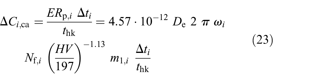
The cavitation degradation rate ( $E{R}_{\mathrm{p},i}$ ) is multiplied by the time period analyzed ( $\mathrm{\Delta }{t}_i$ ) to obtain the increase in wear depth. Dividing this value by the impeller blade thickness ( $t_{\mathrm{hk}}$ ), which represents the maximum allowable wear depth, then yields the decrement of the condition number as caused by cavitation $\mathrm{\Delta }{C}_{i,\mathrm{ca}}$ in the $i^{\mathrm{th}}$ time step. Note that the dimensionless condition number $C$ now represents the relative condition on a scale from 1 (no damage) to 0 (completely degraded or failed).

For the second failure mechanism, that is, erosion, the degradation rate was obtained from equation (17). As the experiment in Serrano et al. ⁴⁵ determined the volume worn in a determined plate area, it is necessary to divide the worn volume by the analyzed area ( $1\mathrm{c}{\mathrm{m}}^2$ ) to obtain the wear depth of the plate. Also for this model the degradation is transformed to a dimensionless condition number by dividing the wear depth by the blade thickness ( $t_{\mathrm{hk}}$ ). Thus, the following expression for the decrement of the condition number caused by erosion ( $\mathrm{\Delta }{C}_{i,\mathrm{er}}$ ) is obtained:

$$\mathrm{\Delta }{C}_{i,\mathrm{er}}=\frac{k_i{F}_{\mathrm{D},i}{V}_{\mathrm{r},i}\mathrm{\Delta }{t}_i{10}^3}{A_{\mathrm{b}}{t}_{\mathrm{hk}}}$$

(24)

Finally, equation (25) represents the decrement of the condition number caused by corrosion ( $\mathrm{\Delta }{C}_{i,\mathrm{co}}$ ). As aforementioned, an equation that could cover all situations for corrosion is not available. Besides, for different used materials, the corrosion rate differs significantly. Therefore, the parameter ${\omega }_{\mathrm{co},i}$ represents the corrosion rate in terms of corrosion depth per time unit ⁵¹ and $\mathrm{\Delta }{t}_i$ is the time period analyzed. The change in impeller condition (due to corrosion) is again obtained by dividing the corrosion depth by the wall thickness ( $t_{\mathrm{hk}}$ ):

$$\mathrm{\Delta }{C}_{i,\mathrm{co}}=\frac{{\omega }_{\mathrm{co},i}\mathrm{\Delta }{t}_i}{t_{\mathrm{hk}}}$$

(25)

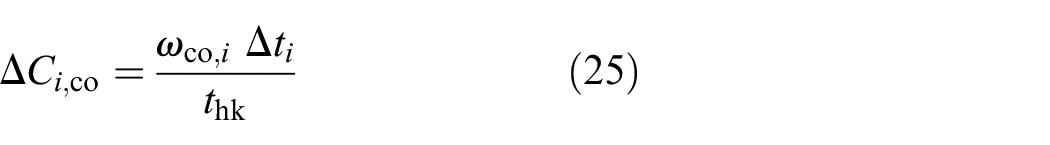
The next step is to integrate the three separate models into the new model, which is denoted the Physical Combination Model (PCM). The process to calculate the impeller condition consists of the steps as presented in Figure 9. For the input of the process, two sets of parameters are used. Some parameters are constant for the operational period ( $x$ ), that is, the usage data related to the installation or design. The other group of parameters varies over time, where sensors usually provide the values. These parameters, load data, also define the number of iterations ( $n$ time steps). In each iteration ( $i$ ) the cavitation, erosion, corrosion, and accumulated degradation $\mathrm{\Delta }{C}_i$ are calculated. $\mathrm{\Delta }{C}_i$ is subtracted from the previous value of the impeller condition $C_{\mathrm{imp}}$ . In this way, $C_{\mathrm{imp}}$ decrease from 1 (blade without degradation) to 0 (impeller completely degraded). Figure 8 presents the degradation scale from green to red, as also will be used on the y-axis of all figures presenting the impeller lifetime in section “Comparison of different models.” Note that at a condition value of 1 the impeller is new and smooth, and the pump will show optimal performance and efficiency. The condition “completely degraded,” $C_{\mathrm{imp}}$  = 0, indicates that the most affected area is completely worn away, that is, a hole appears in the impeller wall. Although it is known that at this point the pressure head or pump efficiency starts to drop substantially, ⁵⁵ it does not yet imply that the pump stopped working completely.

Figure 8.

Degradation scale.

After analyzing the load case $x$ , the Impeller Condition at the end of period $x$ ( $C_{\mathrm{imp},x}$ [−]), the accumulated operational time ( $t_{\mathrm{ac}}$ $\left[\mathrm{operational}\mathrm{hours}\right]$ , equation (27)) and the average degradation rate during the operational time for the target case $\overline{{(\mathrm{dC}/\mathrm{dt})}_x}$ [−], equation (28) are obtained.

The decrease of the condition number by each failure mechanism is represented by equations (23) until (25). It is assumed that several operational conditions ( $x$ ) will occur, in which the loads (e.g. flow, pressure, contamination, etc.) are not constant, and are therefore covered by $n$ time steps, while the configuration data (e.g. installation, tube length, etc) are constant. The actual impeller condition at the end of load case $x$ ( $C_{\mathrm{imp},x}$ ) is obtained by subtracting the accumulated degradation ( $\mathrm{\Delta }{C}_i$ ) from the previous impeller condition ( $C_{\mathrm{imp},x-1}$ ). The accumulated operational time ( $t_{\mathrm{ac},x}$ ) is obtained by adding the previously accumulated operational time to the sum of the $n$ time steps ( $\mathrm{\Delta }{t}_i$ ), in load case $x$ , see equation (27). Equation (28), finally, represents the average degradation rate during load case $x$ .

$$\begin{array}{c}\multicolumn{1}{c}{C_{\mathrm{imp},x}=C_{\mathrm{imp},x-1}-\sum _{i=1}^n\mathrm{\Delta }{C}_i}\\ =C_{\mathrm{imp},x-1}-\sum _{i=1}^n(\mathrm{\Delta }{C}_{i,\mathrm{er}}+\mathrm{\Delta }{C}_{i,\mathrm{ca}}+\mathrm{\Delta }{C}_{i,\mathrm{co}})\hfill \end{array}$$

(26)

$$t_{\mathrm{ac},x}=t_{\mathrm{ac},x-1}+\sum _{i=1}^n\mathrm{\Delta }{t}_i$$

(27)

$$\overline{{(\mathrm{dC}/\mathrm{dt})}_x}=\frac{{\sum }_{i=1}^n\mathrm{\Delta }{C}_i}{{\sum }_{i=1}^n\mathrm{\Delta }{t}_i}$$

(28)

The process in Figure 9 is related to one load case $x$ in the Physical Combination Model (PCM) process. Initially, $C_{\mathrm{imp}}$ is one, which means that the impeller is new and without degradation. The same process is repeated for all load cases, see Figure 10. After that, the procedure verifies whether the $C_{\mathrm{imp},x}$ is already zero, which means that the impeller achieved the end of its lifetime. If the $C_{\mathrm{imp},x}$ is still larger than zero, the physical combination model process can be applied to a next or future operational condition. In this evaluation, it is checked whether the actual/future case is the same as any past case. If so, the average wear from the past case can be used to save computation time. If the operational condition was not experienced before, the PCM process is executed with the actual/estimated parameters, that usually consist of data for a new configuration, and an estimation of the load parameters. This procedure is executed until the $C_{\mathrm{imp},x}$ is zero. Then the accumulated operational time ( $t_{\mathrm{ac},x}$ ) represents the component lifetime.

Figure 9.

Physical combination model process.

Figure 10.

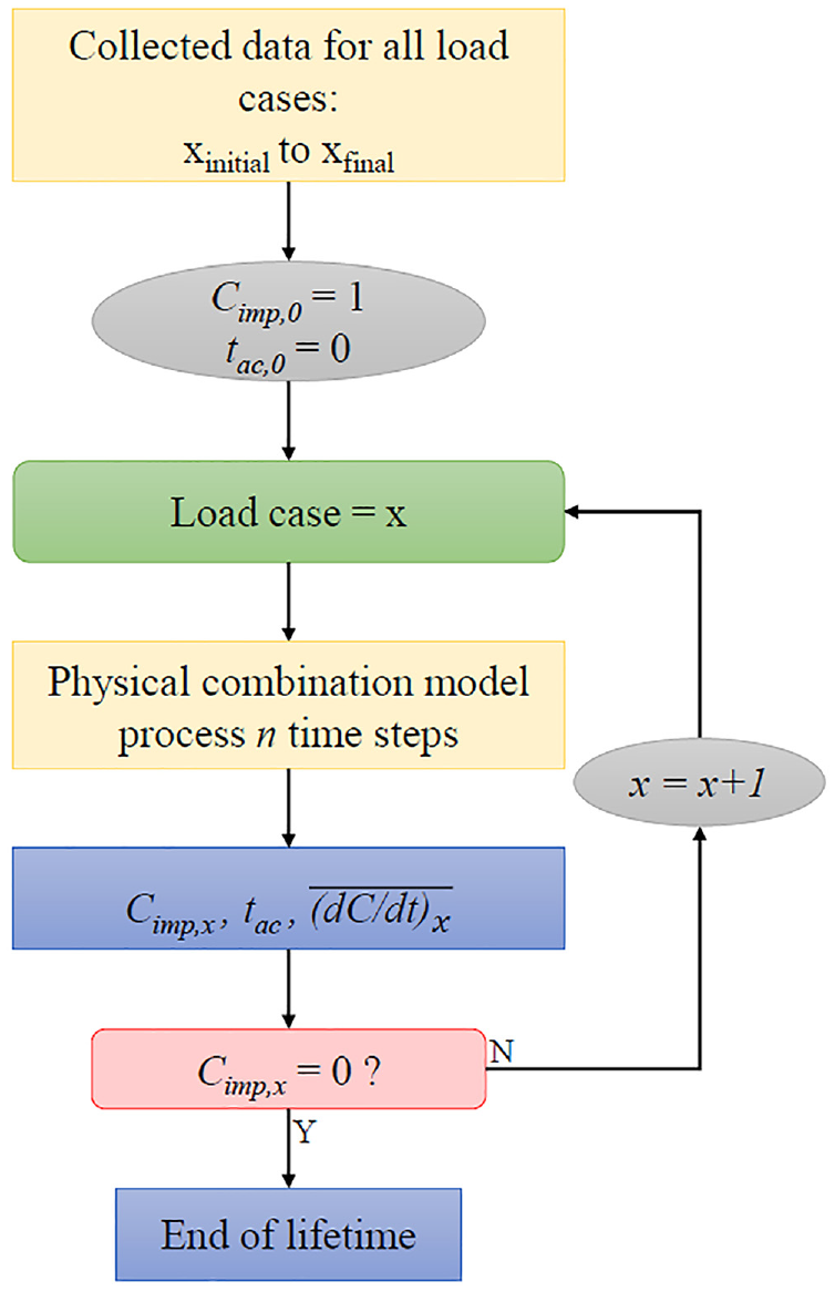
Flow diagram for the physical model combination process.

The methodology proposed here is applied in the next section. The proposed combination of physical and empirical models is compared to the reference failure rate model as well as to the separate cavitation model as modified by Hattori and Kishimoto. ²⁴

Comparison of different models

For this case study, data from a seawater pump NISM 125-250/01 was analyzed. ⁵⁶ The sensors mounted on this pump measured pressure and temperature over time, thus providing a description of the operating history of the pump. Other characteristics as installation and flow were estimated based on a practical application. The base failure rate, used in the failure rate model, was obtained from the OREDA database. ³⁶ These assumptions were necessary due to the difficulties in finding a case with all the required data. Table 1 specifies all the parameters used in this work with the respective references. Note that for all parameters a reference value is given, and for many parameters also the range over which these parameters typically vary (defined by a minimum and maximum value).

Table 1.

Reference, minimal, and maximum parameter values used in the case study.

Param.	Ref Val.	Min Val.	Max Val.	Unit	Reference
λFD,B	4.85	2.425	7.275	f./Mhrs*	Silveira et al. 42
Q	est.(p)**	1	400	m3/h	Silveira et al. 42
Q r	400	–	–	m3/h	Silveira et al. 42
V O	1750	1700	1800	m/s	Silveira et al. 42
F AC	32	1	128	µm	Silveira et al. 42
CSF	1.5	1	2	–	Silveira et al. 42
D e	0.035	–	–	m	Approximate
ω	29.17	28.3	30	s−1	Silveira et al. 42
HV	200	–	–	HV	AMPCO 57
H SV	f(Q)***	2	14	m	Janse 56
Q d	260	–	–	m3/h	Janse 56
H	f(Q)***	10	24	mmHg	Janse 56
h b	760	–	–	m	Rafferty 58
S.G.	1.026	–	–	–	Strachan 59
h	−1	–	–	m	Case study
Z	9	1	9	m	Case study
g	9.81	–	–	m/s 2	–
h vp	0.0229	0.0064	0.042	bar	ITTC 60
f	0.018	0.01	0.1	–	Takacs 61
L tube	1.5	–	–	m	Case study
D tube	0.2	–	–	m	Case study
T	Value	273.15	308.15	K	Read value
p u	0.46	–	–	MPa	Hattori et al. 44
p v	0.0023	0.00064	0.0042	MPa	ITTC 60
S c	0.75	0.5	1.5	g/l	Lauwaert et al. 62 ; Green et al. 63
ρ	1024	1021.8	1028.1	kg/m3	ITTC 60
V r	f(Q)***	13.85	24.23	m/s	Korpela 46
A b	0.0012	–	–	m2	Approximate
r 2	0.12	–	–	m	Approximate
ν	1.051E-06	8.43E-07	1.79E-06	m2/s	ITTC 60
wco	0.1	0.01	1	mm/year	Janse 56 ; Gülich 51
t	5	–	–	s	Read value
t hk	7.8	–	–	mm	Approximate

*

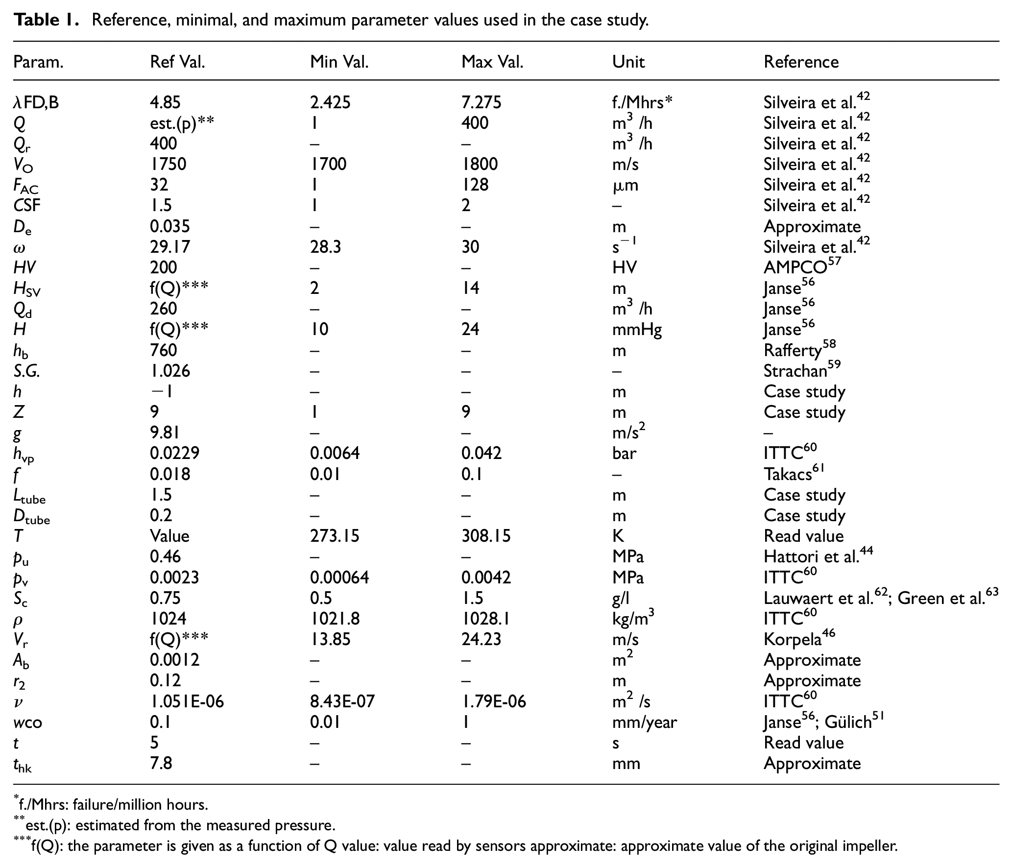
f./Mhrs: failure/million hours.

**

est.(p): estimated from the measured pressure.

***

f(Q): the parameter is given as a function of Q value: value read by sensors approximate: approximate value of the original impeller.

The assumptions for the data that was used for the corrosion mechanism is based on an empirical model. The data is for G-CuAl10Ni material operating with seawater. ⁵⁶

Model implementation

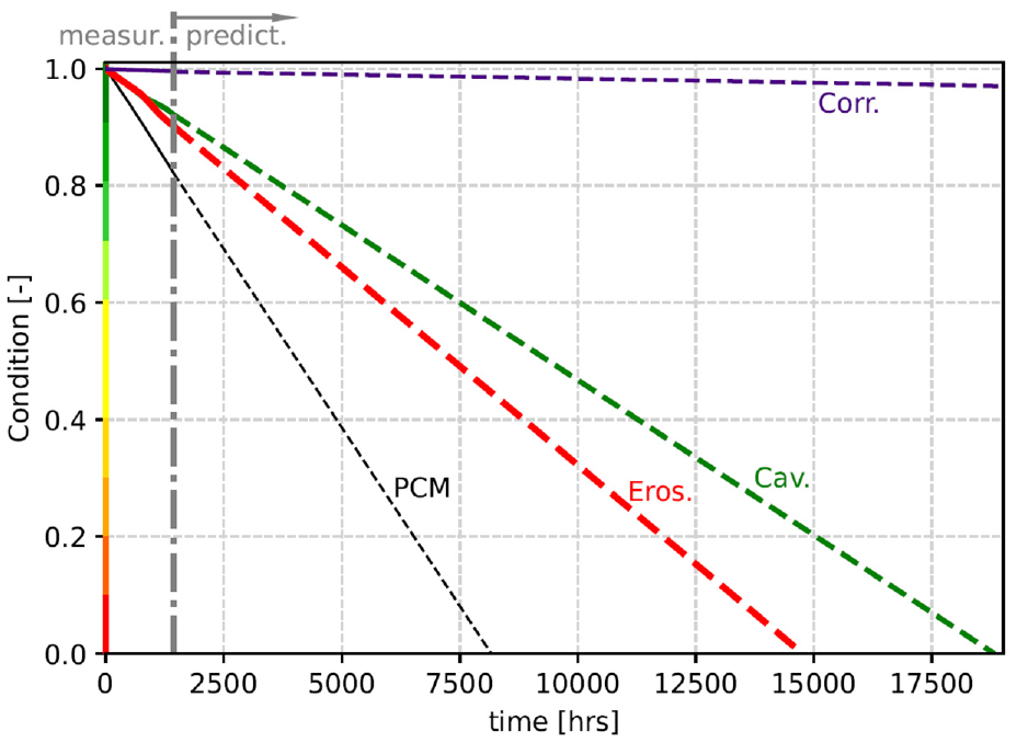
The first step for analyzing the case is applying the proposed model combining the failure mechanisms discussed in section “Integrated life prediction model.” In the result plots, the condition of the impeller will range from 1, representing the initial healthy state to 0, the final and totally degraded state. Figure 11 presents the results of the three failure mechanisms separately, showing the degradation as quantified by the Cavitation model (Cav.), Erosion model (Eros.), and Corrosion model (Cor.). The combined degradation of the failure mechanisms is represented by the Physical Combination Model (PCM); for each time period, the degradation increment was added to the initial state until the end of the measured history was reached, around 2000 h. After that, from this calculated state, a prediction was made by extrapolation, using the average of the degradation increments obtained previously, equation (28). Figure 11 shows that the dominant failure mechanism is erosion, followed by cavitation. It is expected that corrosion has a low degradation rate since it is possible to select a suitable (corrosion resistant) material.

Figure 11.

Evolution of the impeller health state over time under reference conditions, using three degradation models and their combination (PCM): (a) first time period (∼1500 h) based on actual measurements and (b) first time period based on actual measurements, and after that, a prediction (pred.) is made.

Model comparison at the reference condition

The next step in the case study is the comparison of the different models for the reference situation, as specified in the Ref. Val. column in Table 1. Figure 12 presents three different methods to determine the total lifetime for an impeller. First, the physical combination model (PCM), which is the methodology proposed in this work, then the cavitation with aging effect (CavAg) as developed by Hattori and Kishimoto, ²⁴ see equation (5), and finally the traditional failure rate model (FRM), see equation (1). All models are analyzed with the same load, that is, measured data for pressure and temperature, as presented by Silveira et al. ⁴² It is observed that PCM yields the least conservative prediction of the time to failure (∼8100 h), followed by the cavitation aging model (∼7000 h). It is essential to point out that the CavAg model only directly evaluates the end of the lifetime and not the decrease in remaining lifetime point by point as is done in this work. For this reason and due to the aging factor ( $m_2$ , see equation (14)), that it is an exponential equation expressing the aging behavior, the observed parabolic condition decrease of the impeller is not necessary realistic.

Figure 12.

Total lifetime as predicted by different model approaches with reference values.

Table 1. Moreover, as the absolute values of the predicted lifetimes largely depend on the selected parameter values, the best way to compare the three types of models is by normalizing the outputs. After that, different scenario’s can be simulated and the relative changes in response can be compared. Figure 13 represents the lifetime normalization of the three different model approaches for the reference scenario. This is achieved by scaling the time axis with the time to failure for each model separately, yielding fractions of the life time. After the lifetime normalization it is possible to analyze the sensitivity of the models and assess which model better describes the influence of the different scenarios. In the next subsection, various scenarios are simulated and compared.

Figure 13.

Normalization of the total lifetime.

Scenario analyses

In this section, multiple scenarios will be analyzed to identify the sensitivity and response of the proposed PCM model and the other two existing models. The first scenario is varying the sediment concentration in the fluid from 0.75 to 1.5 g/l. The results are presented in Figure 14, showing that the PCM model is the only model that covers this variation in operational condition, as the included erosion model can account for the variation of the sediment concentration. It incorporates the effect of particle size and concentration in the $k$ coefficient, see equation (18b). In that way, the model provides a proper response to the change of operational conditions in this scenario. ⁶⁴ The FRM model does not show any change in predicted lifetime, because the sediment concentration is not covered in this model. The only parameter in the FRM related to particles in the fluid is the filter size, but that is a configuration parameter that does not change with operational conditions (like sediment concentration). Also the CavAg model is unable to quantify this effect.

Figure 14.

Changes in relative lifetime of the impeller due to varying sediment concentration, length of pipe, material, and speed.

The second scenario to be analyzed is the situation with an increase in the length of the pipe preceding the pump. This is a practically relevant scenario, as all installation parameters interfere directly with the component performance and lifetime. ⁶⁵ As observed in Figure 14, $L_{\mathrm{tube}}$ has a larger impact on the relative lifetime when using the Cavitation Aging Model (CavAg) than for the PCM model. This is due to the fact that both models use the same expression to incorporate tube length effects on cavitation, but in the PCM model cavitation is just one of the three mechanisms. The effect of tube length on the total degradation is therefore amplified by the $m_2$ factor for the CavAg model. Finally, the FRM model does not present any change because this model does not include the pump installation into the lifetime prediction.

The change of impeller material in the third scenario impacts various parameters as it affects the material hardness ( $\mathrm{HV}$ ), wear coefficient ( $k$ ), and corrosion degradation increment ( $\mathrm{\Delta }{C}_{i,\mathrm{co}}$ ). This can give misleading results if not all failure mechanisms are considered. For example, in Figure 14 the material was modified from a G-CuAl10Ni (NCI) to GG-25 Gray Cast Iron (GCI). Compared with NCI materials, GCI materials have slightly higher durability and can withstand localized force without deformation. For this reason, GCI materials present a slightly higher relative lifetime regarding cavitation compared with NCI. ⁶⁶ In the cavitation and CavAg models, the hardness is represented by the $\mathrm{HV}$ parameter, 200HV for NCI and 210HV for GCI material. This explains why the relative lifetime increases for a pure cavitation model. However, $k$ represents the wear by the erosion mechanism, and the erosion degradation is higher for GCI than for NCI.^28,67 Besides that, the corrosion degradation is much higher for GCI than for NCI. ⁵¹ All these factors make the relative lifetime for GCI lower than for NCI, as the PCM model correctly shows. The CavAg model therefore presents an unrealistic relative lifetime because it considers only one failure mechanism. The FRM model does not present any change because again no parameter regarding material properties is included in this model.

Lastly, Figure 14 presents the variation in relative lifetime associated to the impeller rotational speed. This parameter is included in all three models analyzed in this work. However, it is observed that the PCM model is more sensitive to this parameter because the speed is affecting all three failure mechanisms.

Degradation during downtime

Another aspect to consider is the degradation in an idle period. Commonly, pumps can be inactive for a while for several reasons, such as scheduled maintenance or the use of a spare pump in a system. During the inactive period, the pump continues to degrade by the corrosion failure mechanism, mainly if the material is not the most suitable for the environment. The PCM methodology is able to cover all scenarios, also when the pump is inoperative. Figure 15 presents the degradation for the case with a downtime. In this case, the material suffers an imperceptible degradation during the 6 months of downtime because the analyzed material is quite resistant to corrosion degradation. Analyses up to 9 years turned out to reveal more visible degradation, even though the material is appropriate for the application.

Figure 15.

Total lifetime prediction with a 6 months inoperative period using a corrosion-resistant material.

In a second scenario, the same period is analyzed, but with a different material. In this case, the studied material is GG-25, the same material analyzed before in Figure 14. Figure 16 presents the degradation, and the jump related to the corrosion failure mechanism during the inoperative period of 6 months is clear. Although the degradation rate in the pump during the downtime period is lower than in active mode, since there is no erosion and cavitation failure mechanism active; it is clearly observed. The downtime degradation is important to be considered because, in some systems, the pump stays idle for a long time, mainly for systems with one or several redundant pumps.

Figure 16.

Total lifetime prediction with 6 months inoperative using an inappropriate material.

Varying scenarios during service life

Another aspect considered in this work is the possibility of changing scenarios during impeller service life. Figure 17 illustrates a case where the sediment concentration during service starts to deviate from the initial scenario, that is, changes from 0.75 to 1.5 g/l. This can occur when the impeller pumps a different fluid or, for example, when a ship goes to a part of the sea with a different sediment concentration. The other parameter values are the same as those in the previous cases. Figure 17 shows a clear change in the slope of the erosion part of the model, while the other two mechanisms are unaffected.

Figure 17.

Load case transition for the various failure mechanisms with a change in sediment concentration after 1432 operating hours.

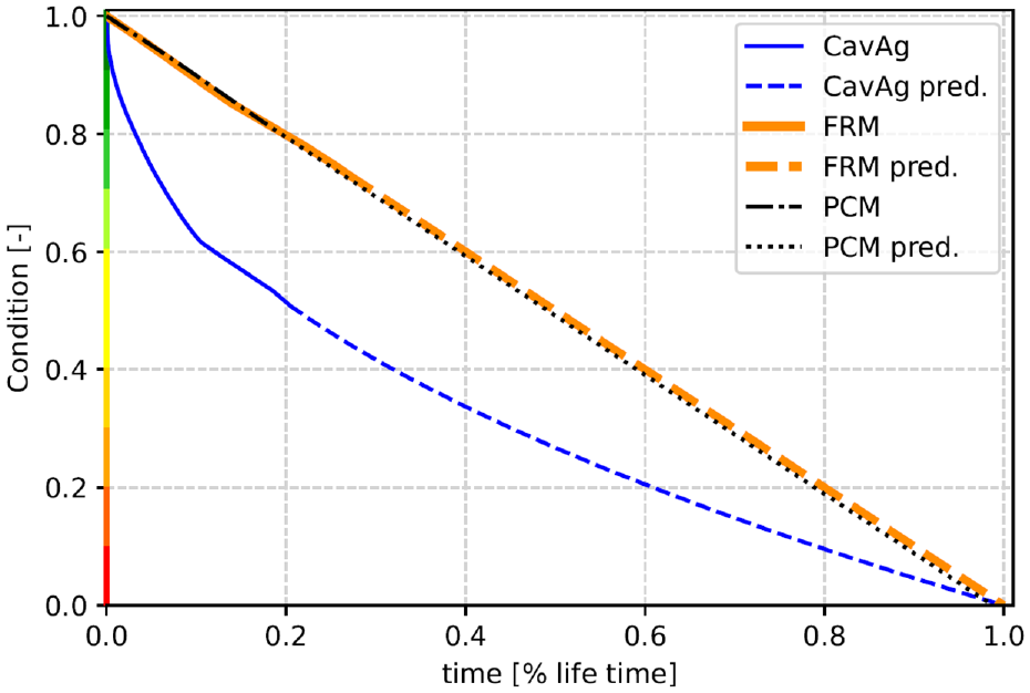
Figure 18 presents the comparison between different models using the case shown in Figure 17. This shows a clear change in slope for the PCM model at the moment the load case changes, while the other two models do not show this response. This is explained by the fact that the FRM and CavAg models have been designed to calculate the failure rate resp. time to failure for a given (constant) load case. The PCM model has been developed to work incrementally in time: the load history is processed in consecutive time steps, allowing to incorporate changes in loads in the degradation calculation. This makes the proposed model much more flexible in calculating the impeller life time for varying operating conditions.

Figure 18.

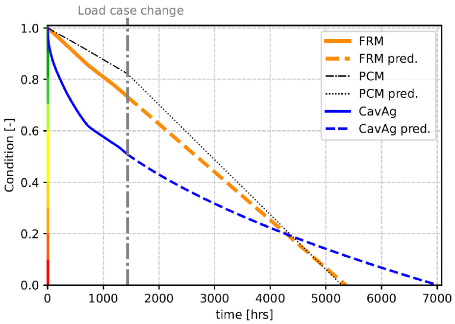
Total lifetime prediction using different model approaches with a change in sediment concentration after 1432 operating hours.

The results from these different scenarios demonstrated the applicability of the proposed methodology. All the failure mechanism and their parameters are considered in the PCM concept, while for the other models, there are some factors without physical meaning, such as the aging effect and base failure rate. Nonetheless, these factors are necessary to adjust the models to a more practical application. The new approach quantifies all the parameters influencing the degradation rate in a meaningful way.

Model development challenges

This section discusses some of the challenges encountered during model development, as well as some assumptions that were necessary for this work. The first stage of this work was to find the main failure mechanisms for the problem “Pump is not functioning properly.” This is not computational and mathematically complex, but it demands specialists to assist in finding the primary failure modes and mechanisms. Otherwise, it can be challenging for someone without knowledge of the component and may demand an extensive literature review. Besides that, a technique developed by Peeters et al. ³³ was used, advising to use FMEA and FTA recursively. This appeared to be effective: otherwise only this process could already be very time-consuming.

The second stage was to identify and understand the available models. Again specific skills are required, in this case, scientific knowledge. The so-called physical models are often not purely physical, and it is necessary to understand the physical phenomena to identify if the equations describe the target failure mechanism. Further, as discussed before, it is important to consider, compare, and evaluate the various models that use different techniques. In this process, some inconsistencies in existing models were discovered. Moreover, models, such as the failure rate model (FRM), may have been built for a specific application, and some modifications are needed to apply these models to other applications.

Another important assumption made in this stage is that the considered failure mechanisms act independently. It is assumed that the occurrence of one mechanism does not affect the degradation rate of another mechanism that occurs simultaneously. This is not always true in practice, as is shown by Alavi Shoushtari. ⁶⁸ Detailed analysis of the casing of a booster pump revealed that the pitted area due to cavitation had a slightly increased surface hardness, which might increase the erosion resistance. On the other hand, the increased surface roughness caused by cavitation increases the erosion wear rate. Although these kind of interactions can always be present, it is assumed here that (i) they only have a minor effect on the degradation rates, and (ii) in most cases one mechanism is dominantly responsible for the degradation rate.

Thirdly, after an extensive model analysis, it is essential to identify the critical degradation area because there is a different degradation rate at different points of the impeller. For this step, it is necessary to investigate the various locations and degradation behavior in relation to the failure mechanisms, which may again require insights from domain specialists.

Finally, the developed methodology has been compared with some established models to assess its performance. Ideally, the prediction results would also be compared to failure data from fielded systems. This is one of the main challenge in the field of (predictive) maintenance, as maintenance aims to prevent failures, and failure data is by definition scarce. Indeed, the authors faced extreme difficulty in finding available cases in the industry. Despite pumps being widely used, and also failing occasionally, the data quality and failure registration is very limited. Also failure data from lab experiments could not be obtained, especially since in open literature no experimental results are available for experiments conducted at real conditions, including phenomena like idle time and irregular flows. Future efforts of the authors will therefore focus both on finding a company case including the relevant data and on developing an experimental set-up that allows for simulating realistic usage patterns.

Another way to assess the predictive performance of the proposed method would be to compare with periodic condition measurements or inspections, that define the momentary condition of the impeller. In scientific literature, several hybrid approaches are available to use Bayesian updating to tune (physical) models with this kind of data, see for example Keizers et al. ⁶⁹ However, in industrial practice, especially for relatively simple systems like pumps, these condition measurements or inspection results are typically not available, and can thus not be used to update or validate the prediction models. Due to this lack of realistic validation data, the authors decided to normalize data to the available case. After that, several scenarios are analyzed, and the relative responses could be compared with the literature.

For most cases, the developed PCM technique had a more realistic response, and proved to be quite sensitive for different scenarios. Also, the scenario with changes in impeller material showed that the proposed model can handle counteracting effects, while in that specific case, the CavAg model presented a change in an unexpected direction. Finally, in most cases, the FRM model does not show any response, indicating that it performs badly in case of changing operational conditions.

Conclusion

In this work, a new methodology for predictive maintenance of centrifugal pump impellers is presented, combining various physical models, analyzing their applicability, and using expert knowledge in a structured strategy. Since the main failure mechanisms are considered, this process can be used for any centrifugal pump impeller application and operational condition. Two other prediction models available in literature, that is, the failure rate model and cavitation model with aging factor, were analyzed and applied to compare with the proposed strategy. The models were simulated in various scenarios, and their response was compared. The developed model presented a more realistic and more sensitive response in the simulated scenarios, considering variations in sediment concentration, pipe length, material, impeller rotational speed, and idle time. Moreover, the proposed method could deliver the lifetime prediction as well as insight in the dominant failure mechanism, which indicates the process that most degrades the impeller. Finally, it was demonstrated that the new proposed model can predict the impeller life time under varying operating conditions, due to the incremental formulation of the model. For future work, the authors recommend that the proposed methodology be demonstrated on a real industrial case or a lab-scale experimental set-up. Furthermore, a fractographic analysis is recommended to verify the dominant failure mechanism and the location of the affected areas.