
Abstract
Functionally Graded Material (FGM) plate is a complicated structure with complex allocation of spatially changing proportions of ceramic and metal within the matter. Various analytical and numerical methods have been applied with a view to evaluating the critical load of FGM plate. However, these conventional methods struggle when the computational complexity is significant, which represents an obstacle to incorporation with other advanced techniques where computational power is required (e.g. optimization or random simulations). The Neural Network (NNet) model has been successfully applied to resolve this issue. However, the conventional NNet requires proper configuration to take advantage of the model, and thus, careful parameter tuning is required. Furthermore, the NNet is typically a “black box,” where the prediction mechanism is hidden. This paper establishes an optimized architecture for NNet, with parametric study of the model’s hyperparameters. Variance propagation is also applied to observe the variation of the model’s performance on random sub-databases splintered from the database. To this end, the explicit expression of the trained NNet model is provided after mathematically deploying the hidden algebra behind an NNet prediction. The developed model has very promising evaluation metrics: R2, MAE, and RMSE on the test set are 0.999925, 0.067516, and 0.146438, respectively.
Introduction
Originating in Japan in the 1980s as thermally resistant material for aerospace vehicles,1,2 Functionally Graded Material (FGM) plate is an advanced structure which has a spatially changing mixture of ceramic and metal constituents. This mixture improves the material’s fire resistance and stiffness, due to the inclusion of ceramic as compared to a purely metal material. Conversely, the ductility of metal compensates for the brittleness of ceramic. The history of the FGM and its applications are detailed in Jha et al. 3 More details on the theories of modeling and analysis of functionally graded plates and shells can be found in Thai and Kim 4 and Thai et al. 5 Besides, a summary of literature review on vibration characteristics of plates can be found in Zarastvand et al.6,7 Last but not least, sound propagation analysis of plate structures is well documented in Ghafouri et al. 8 and Talebitooti et al. 9 Additionally, the FGM’s modeling and analysis were also reviewed by Birman and Byrd. 10
FGM, with the advantages listed above, has been attracting the interest of many researchers, with various theories and techniques applied. To comprehend the buckling behavior of FGM plate, both conventional analytical methods and numerical methods have been applied. 11 A wide range of mathematical and mechanical methods have been used to analyze FGM plates. First-order shear deformation is a critical method that is widely accepted.12–15 Higher-order versions of this method have subsequently been applied, in publications such as.16–19 Various problems related to FGM buckling analysis have also been published, such as the critical load of FGM under mechanical and thermal load cases.14–16,20 The structures’ nonlinearity also affects matters such as load types 20 ; geometry,19,21 imperfection,20,22 and material.23,24
The approaches conventionally applied are advanced methods which require interactions and continuously solving matrices, especially for the cases where FE methods or nonlinear problems are involved. As a result, these approaches are computationally expensive, including in terms of the speed and memory required. Consequently, to further incorporate these models with advanced techniques requiring integrations is no easy task.25,26 A data-driven approach has been shown to be helpful in addressing these difficulties. A machine-learning model such as Artificial Neural Network, NNet, is a sensible choice, provided databases are available. NNet has often been applied to predict the mechanical behavior of FGM structures.21,26–28 Duong et al. 26 used Monte Carlo simulation to stochastically assess the critical buckling load for FGM plate. The paper noted that FE or analytical models were unable to cope with the millions of predictions required. Khatir et al. 21 proposed a two-phase approach: the Frequency Response Function is applied in the first stage to predict the failure elements, and an Improved Artificial Neural Network is subsequently run to predict damage level through a range of indicators. The vibrating characteristics of FGM plates, resting on an elastic foundation is predicted using NNet and the FEA database in Tran et al. 27 Abdeen and Bichir 28 developed an NNet model to predict the deflection of FGM plates supported by fluid matter.
However, finding a proper architecture for the NNet requires careful hyper-parametric tuning 29 or advanced techniques. 30 The user must also possess advanced knowledge and skills. In addition, a problem arises when applying NNet – the implicit expression of the predicting process, commonly known as a “black box.” This leads to difficulty for practical engineering applications. Consequently, there is a desire for the explicit expression of the NNet model or an empirical model. Many research projects have been published, with a view to developing a semi-data driven and semi-analytical model; the aim is for the final result to be a solid equation for predicting the variable of interest with optimized factors.31–33 These models have the obvious advantages of being explicit and requiring least computational effort. Phan et al. 31 use pre-fixed equations with changeable factors, and optimize them by minimizing the error between simulated and predicted outputs. The authors later developed their study with Phan et al., 32 developing an empirical model to predict defective pipe moment capacity, with 49 factors. The advantage of such an approach was also applied to improve the accuracy of the Folias factor for the same problem. 34
This paper has a similar aim: to develop a ready-to-use model to predict critical load for FGM plate. Specifically, the results of the hidden mathematical operations in the network are explicitly provided in the equation format, making it practically applicable for users who have no advanced knowledge of ML or coding skill. The database employed in developing the model is derived from the fundamental analytic method, whilst the NNet architecture is obtained by hyper-parameter tuning. The dependence on model variance and on the database are investigated by variance propagation.
Materials and methods
Ultimate load of functionally graded structures
The dimensions of the plate used in this study are given in Figure 1: its width, a; length, b and thickness, h. As discussed above, FGM is a mixture of metal and ceramic, with proportions differing along the thickness of the plate (e.g. z-axis).

Diagram of FGM plate in the coordinate system.
Consequently, the overall Young’s modulus of the FGM, E, is z-axis dependent. The relationship with the Young’s moduli of metal and ceramic (Em and Ec, respectively) can be quantified as shown in equation (1) 35 :

where p is the positive volume fraction exponent; and υ is the Poisson’s ratio.
Based on first-order shear deformation theory (FSDT), the critical load of a simply supported plate can be found by solving equation (2). 26

where K is the stiffness matrix of the FGM plate. K can be expressed as in equation (3), with


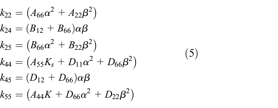
where:
-
- k is the axial load factor on the x and y axis, (i.e.

-

- Ks is the factor of the transverse shear correction (chosen as 5/6 38 ).
The dimensionless critical load

By randomly generating inputs, including k, p, b/h, a/b, and Ec/Em and solving equation (8) for
Characteristics of the database.

Methods used
Neural Network and its architecture
One tool that is commonly employed for data-driven operations is Neural Network (hereinafter called NNet, for short). The technique was developed by McCulloch and Pitts 40 in 1943, aiming to emulate the biological neural network found in human brains. Thus, NNet’s architecture is an inter-connected set of artificial processing elements (i.e. artificial neurons), arranged in layers or vectors, that carry out computational tasks for the problem at hand. 25 To simulate the synapses of the human brain, an NNet model is constructed including inputs, variable weights and outputs (these are similar to the dendrites, cell bodies, axons, and synapses in the human brain). NNet displays crucial benefits over the classic computational techniques that are most commonly used. Firstly, NNet does not require any pre-constraints or hypotheses during the learning phase. Unaided, the model is able to detect complex and nonlinear relationships within the database. From a computational standpoint, NNet is extremely powerful for high-dimensional problems, thanks to its capability to carry out processing tasks in parallel.
An NNet model is composed of three basic parts: the input layer, the hidden layer(s) and the output layer. In this study, a one-hidden-layer NNet model was chosen to predict the critical load of functionally graded material plates. The architecture is illustrated in Figure 2. For such an architecture, the NNet model computes the following nonlinear function 41 :

where f is the nonlinear function, X is the vector of independent variables of dimension N and Y is the vector of dependent variables of dimension M. Like the asynchronous activity of the human nervous system, the artificial neurons can also be activated with the weighted input signal in an asynchronous manner. In other words, the weights and bias of each neuron are adjusted to identify the optimal set of parameters for the model. Mathematically, the function f in equation (9) is expressed below for the problem in question 42 :

Firstly, fh, W, and b are the transfer function, weight matrix, and bias for neurons in the hidden layer. Secondly, fo, M, and bo are the transfer function, weight matrix, and bias for neurons in the output layer. These parameters are also represented in Figure 2.
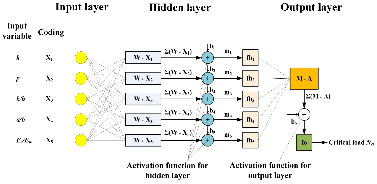
One-hidden-layer architecture of the NNet model considered in this study, including five inputs and one output.
In this case, m is computed as:

The procedure for computing weight and bias for neurons in the model is called the “learning phase.” Typically, learning employs an optimization technique (in this study, it uses backpropagation as a gradient computing method43,44). More specifically, the optimizer searches for the minimum cost function based on gradient descent, while the backpropagation computes the gradient for the optimizer to employ. For a specific problem, it is very hard to directly identify which transfer function, learning algorithm and cost function are most appropriate. The choice depends on numerous factors – for instance, the nature of the prediction problem, the size of the dataset, the size of the hidden layer and the error target. 45 Consequently, in this work, a parametric run was designed and performed to identify the most suitable specifications for the NNet architecture. Thus, transfer function, cost function, learning function and number of neurons in the hidden layer are described below for the parametric run.
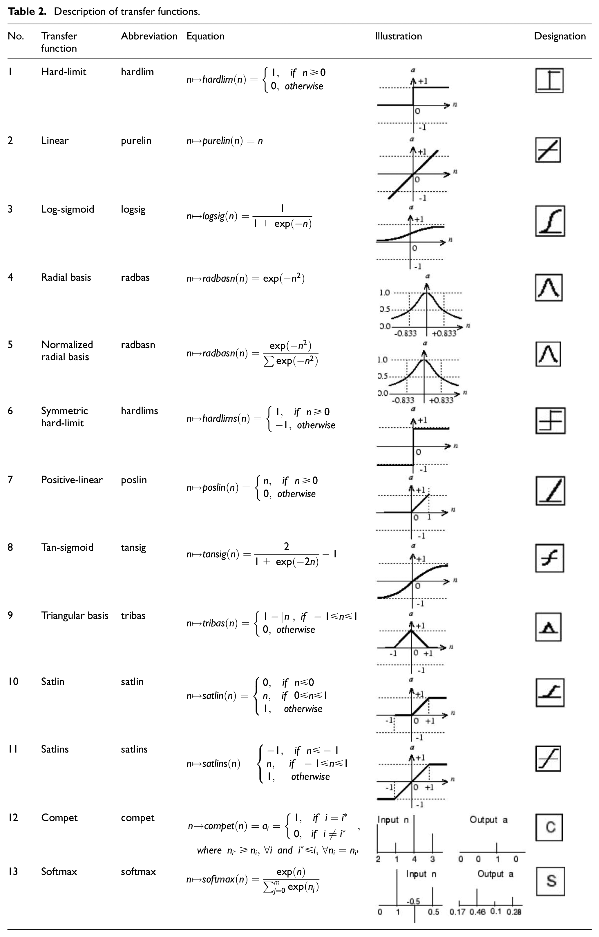
In this work, 13 transfer functions were considered; Table 2 gives their name, abbreviation, equation, illustration and designation. In addition, 11 backpropagation learning algorithms were employed, listed in Table 3 including their name, abbreviation, characteristics, drawbacks and reference. Next, three cost functions were used: mean squared error (MSE), mean absolute error (MAE), and sum absolute error (SAE). Finally, the number of neurons in the hidden layer ranged from 1 to 35.
Description of transfer functions.
Activation functions used.

This study optimizes the NNnet model and also opens up the “black-box” machine-learning technique for practical applications. To this end, the weights and biases of the optimized NNet model are appended to this manuscript, including a closed-form prediction equation.
Monte Carlo simulation and statistical convergence
The Monte Carlo method was chosen for this study to investigate the impact of input variability on response via prediction models (see Figure 3). This technique has several advantages in terms of generation, 58 parallelization, 59 and numerical analysis. 60 The technique works by repeatedly and randomly generating a set of variables, each of which follows a different probability density function. 61 As a result, variability and uncertainty in the input may be transferred to the output via the numerical model. However, several statistical convergence indicators must be incorporated in order to regulate the number of realizations. In this study, statistical convergence was controlled as a function of the mean and standard deviation for a given random variable. The mean estimator is based on the equation below62,63:

where


Diagram of Monte Carlo method.
Statistical quality metrics
The statistical quality evaluation metrics used in this study are Coefficient of determination, Mean squared error, and Root mean squared error. Details of these metrics and their expressions are provided in Table 4 below.
Details of statistical metrics of quality used in this study.

Methodology
The methodology flowchart is represented in Figure 4, including the six main steps as below:

Methodology flowchart.
Results and discussion
Optimization of model
Results of parametric study
In this section, the optimal number of hidden neuron layers is identified. It is worth noting that other parameters – learning function, transfer function and cost function were retained as Levenberg-Marquardt, tansig, and mean square error, respectively (default parameters). Figure 5(a)–(c) show the distribution (mean and standard deviation) of RMSE, MAE, and R2 respectively, as a function of the number of neurons, which was varied from 1 to 35 with a step of 1. Such line plots with error bar highlight the probability distribution of statistical metrics over 2000 random runs. Figure 5 reveals that a low number of neurons (i.e. fewer than 5) provided an unsatisfactory predictive performance, with respect to all statistical quality metrics. Next, Figure 5 also indicates that the predictive performances converge if the neuron number is higher than 30. This observation indicates that there is an optimal neuron number for the problem at hand (i.e. increasing the number of neurons does not significantly improve model performance beyond a certain threshold). In addition, the results were similar using both the training and testing datasets. It is apparent that no overfitting occurred during the training process, as the two curves correlate closely. Moreover, the higher the number of neurons, the smaller the deviation of statistical metrics – especially in the case of R2, as seen in Figure 5(c). This point confirms that the performance of NNet depends heavily on variability in the input space, for fewer than 15 neurons in this case. Finally, 30 was chosen as the optimal neuron number.

Parametric study as a function of neuron number: line plot with error bar (mean and standard deviation values) for (a) RMSE, (b) MAE, and (c) R2. Both training and testing data points are represented.
Figure 6 presents the optimization process for the NNet model’s training algorithm. Other parameters – transfer function, neuron number and cost function – were kept as tansig, 30 (as identified previously) and mean square error, respectively. Figure 6(a)–(c) show the evolution of RMSE, MAE, and R2, respectively, as a function of the learning algorithms shown in Table 3. Similar to Figure 5, the probability distribution of statistical metrics over 2000 Monte Carlo random runs is presented through mean and standard deviation (line plot with error bar). The performance was classified based on the mean value of the histogram. The results in Figure 6 indicate that the LM algorithm outperformed other functions, considering all metrics R2, RMSE, and MAE. Moreover, the LM function also generated the smallest standard deviation (i.e. slightest fluctuation). Based on these observations, the LM function was chosen as the best training algorithm.

Parametric study as a function of training function: line plot with error bar (mean and standard deviation values) for (a) RMSE, (b) MAE, and (c) R2. Both training and testing data points are represented.
This section discusses how different transfer functions affect the performance of the NNet model. The other parameters – learning function, neuron number, and cost function – were set to Levenberg-Marquardt (as previously found), 30 (as previously identified), and mean square error, respectively. Figure 7(a)–(c) depict the line plot with error bar distribution of RMSE, MAE, and R2 as a function of the 13 transfer functions utilized. In Figure 7, mean and standard deviation values depict the probability distribution of statistical measures over 2000 random sample runs. The performance was classified based on the distribution’s mean value. The results showed that the logsig, tansig, and softmax functions performed better for the NNet model, particularly the softmax function. As a result, the softmax function was ultimately picked as the best.

Parametric study as a function of activation function: line plot with error bar (mean and standard deviation values) for (a) RMSE, (b) MAE, and (c) R2. Both training and testing data points are represented.
Figure 8(a)–(c) show the line plot with error bar distribution of RMSE, MAE, and R2, respectively, as a function of the three cost functions used. However, it can be seen that there is no remarkable difference between these three functions. Thus, MSE was finally chosen.
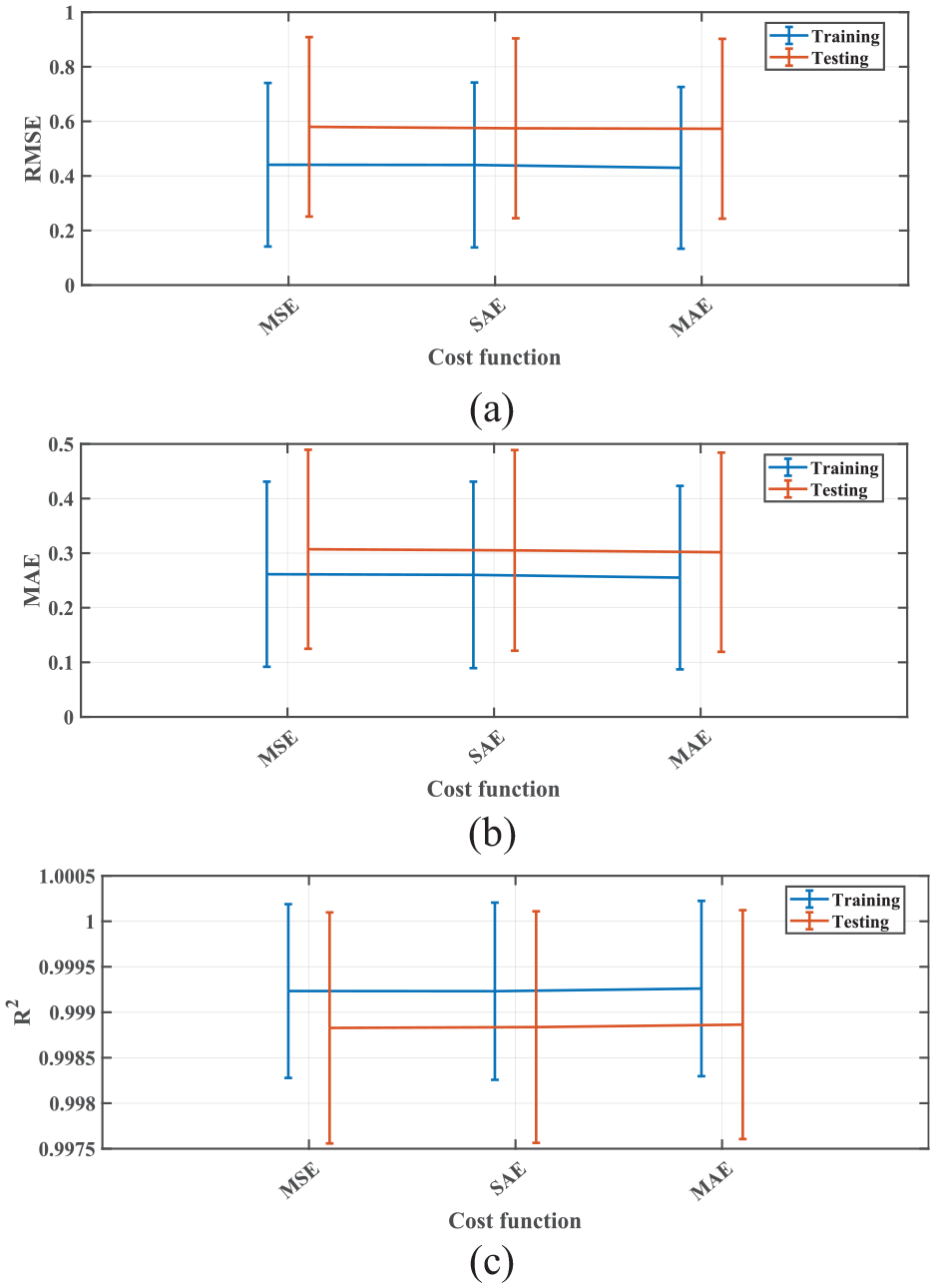
Parametric study as a function of cost function: line plot with error bar (mean and standard deviation values) for (a) RMSE, (b) MAE, and (c) R2. Both training and testing data points are represented.
Convergence of random sampling
The variability derived from the randomness of the database is investigated and partly eliminated by variability propagation. For this technique, random sampling is used with 70% of samples in the database, and the NNet model is developed for a number of runs with sub-databases. Model errors (RMSE and MAE) of various NNet architectures/models are recorded, each being “fed” with only (70% samples) × (number of runs) in the database). It can be observed from Figure 9 that the errors for each run exceed their mean, µRMSE and µMAE (see equation (12) for the definition of such statistical convergence), on both the training and testing dataset of all the models, converge with up to 2000 runs. Meanwhile, the standard deviation of errors, σRMSE and σMAE (see equation (13) for the definition of such statistical convergence), converge with around 500 runs and vary stably thereafter. Finally, it may be said that 2000 random realizations are necessary to achieve statistically reliable results in terms of both mean and standard deviation values.
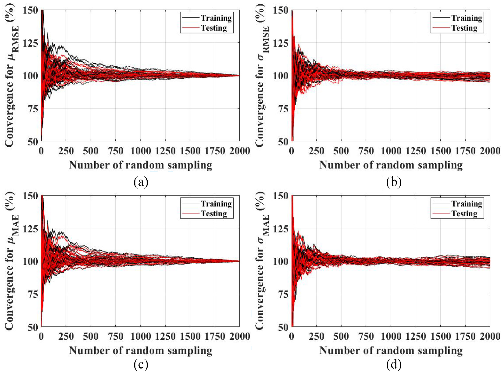
Statistical convergence of Monte Carlo simulations, with respect to the mean value of (a) RMSE, (b) MAE, and the standard deviation of (c) RMSE, (d) MAE. Both training and testing data points are represented.
Optimal parameters
The ideal parameters of the NNet model are shown below based on the previous results:
Number of neurons in hidden layer: 30
Transfer function for hidden layer: softmax
Training function: LM
Cost function: MSE
Prediction capability of optimized model
Model evaluation
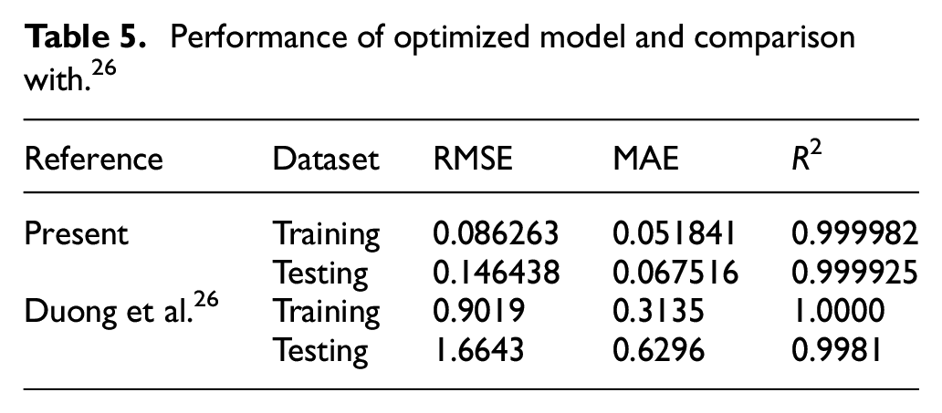
Based on the parametric study presented above, the best NNnet model was identified and the evaluation metrics for the model are provided in Table 5. It can be seen that the model performs well; the errors between the predicted and actual values are slight on both the training (RMSE = 0.086263 and MAE = 0.051841) and testing datasets (RMSE = 0.146438 and MAE =0.067516). Also, the R2 values almost reach the absolute value of 1.0. Compared to the non-optimized model from, 26 the present model is considerably more accurate, with the errors around 10 times less than those found by Duong et al. 26 The difference between MAE on the training and testing dataset is also reduced from roughly 50% (i.e. 0.6296 vs 0.3135) to almost equal (i.e. 0.051841 vs 0.067516).
Performance of optimized model and comparison with. 26
Figures 10 and 11 illustrate the actual values and those predicted by the NNet model developed in this study. In Figure 10, all data points are concentrated along the ideal line which almost overlaps the linear fit, using both the training and testing data points. This implies near perfect prediction by the developed model. Also, the ordered outputs versus the actual data in Figure 11 show insignificant differences with the range of outputs from the database. This indicates that no localized area has a significantly greater error than the rest.

Regression analyses using: (a) training data and (b) testing data.

Comparison as a function of sample index for: (a) learning data and (b) testing data.
Local analysis of performance at different quantile levels
This section presents an analysis of the prediction performance of the optimized NNet model at local quantile levels. For this purpose, nine quantile levels discretized from 10% to 90% with a resolution of 10% of the probability distribution, for both the predicted and actual dimensionless critical load

Comparison as a function of quantile levels for: (a) learning data, (b) testing data, and (c) all data.
Comparison as a function of quantile levels.

Computational time
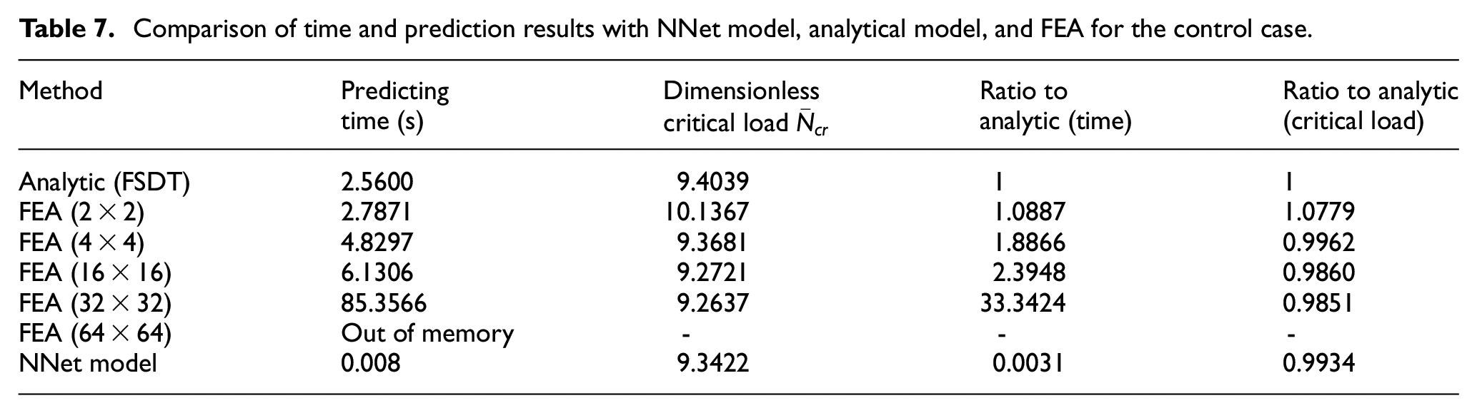
Investigations of the computing velocity of the analytic model (with FSDT), FEA and NNet models are briefly provided in Table 7. It can be seen that to obtain the prediction, the NNet model requires only 0.008 s, compared to 2.5600 s for the analytic model and 4.8297 s for FEA (to have an acceptable value with 4 × 4 elements). There is a significant time saving by using the NNet model. For the FEA, the results can be difficult to reach due to lack of memory or the overly coarse meshing system. This difference is crucial for the incorporation of a critical load model and other advanced techniques which require a large number of predictions, such as optimization. Indeed, an optimization problem can be applied to search for the optimal material properties of the plate that can maximize the critical buckling loads and/or the natural frequencies. It is worth noticing that different mechanical constraints can also be applied. Consequently, if the predicting time is small (for instance, 0.008 s using the NNet model proposed in the present study), the search for the optimal material properties should be much faster.
Comparison of time and prediction results with NNet model, analytical model, and FEA for the control case.
Development of empirical equation and implementation for practical use
In practice, it is not appropriate for researchers and/or engineers to use machine-learning techniques, because of model parameters including weights, biases, transfer functions and others. For the purposes of practical application, the authors open the “black box” of the NNet machine-learning technique, and shine light upon its workings. To this end, the weight and bias of the optimized NNet model are provided and appended to this manuscript, including the explicit mathematic equation of the NNet.
The closed form of the explicit equations for estimating critical load of functionally graded material plate is presented below:

where
For a direct use, the prediction equation (14) was implemented in a practical application developed in Matlab, and appended to this paper. Figure 13 presents a snapshot of the practical application. All interested users can download it and use it to predict the critical load of functionally graded material.
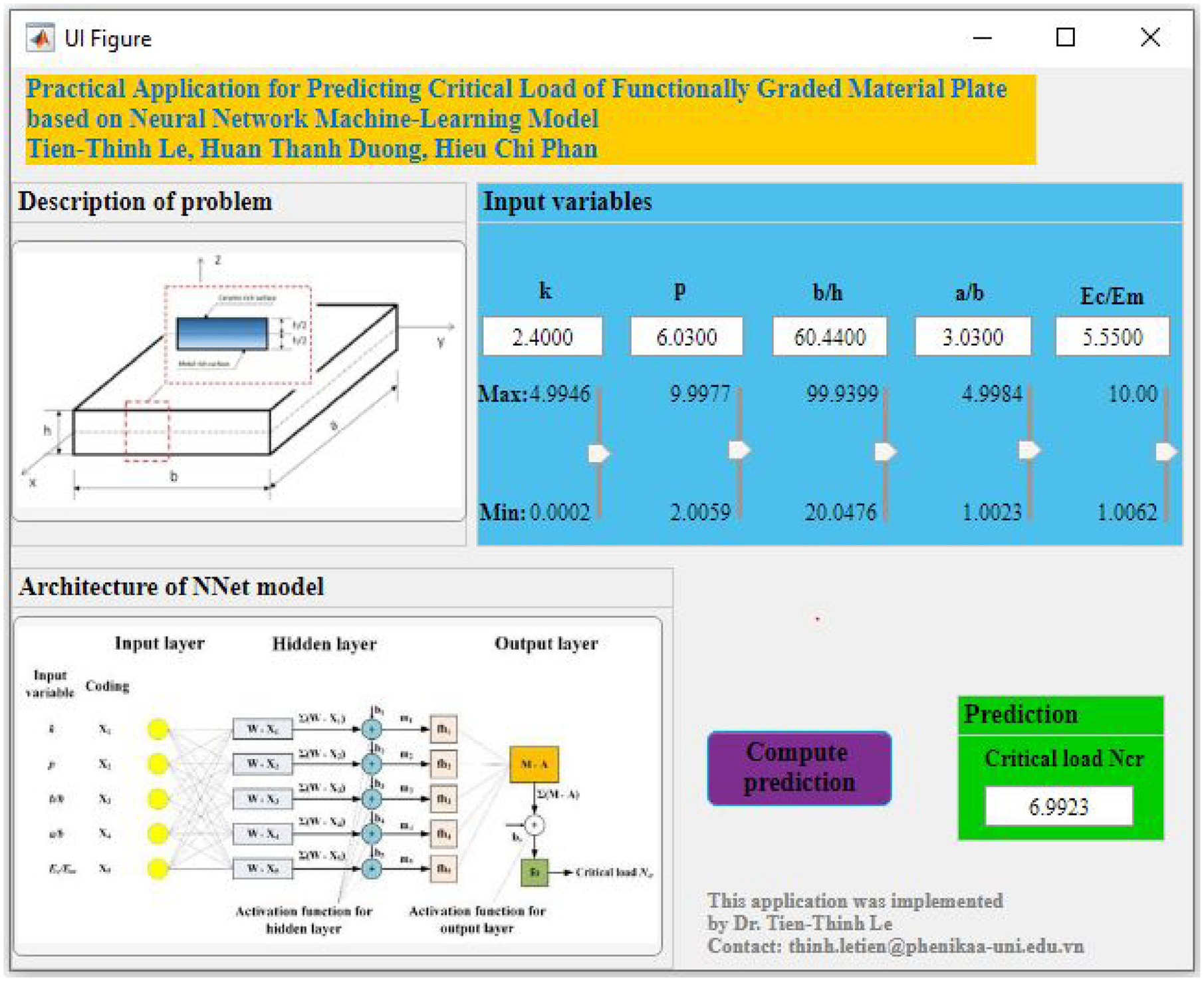
Graphical User Interface of the practical application.
Research significance
The determination of the ultimate load of functionally graded plates has proven challenging for researchers and engineers due to the complex and nonlinear nature of the mechanics involved, which depend on various micro-parameters. Despite numerous theoretical and numerical studies aimed at addressing this issue, a generalized, simple, and robust solution that accounts for all the parameters affecting the ultimate load has yet to be developed. In this study, an artificial neural network is utilized to predict the ultimate load of functionally graded plates. It is noteworthy that the model results in an explicit, robust, and simple prediction equation for practical application. The proposed solution is validated against an analytical approach, and when compared to analytical and finite element methods, the model saves significant computation time. The proposed model can be used to optimize the material properties of the plates to maximize critical buckling loads and/or natural frequencies, taking into consideration different mechanical constraints, due to its faster prediction time compared to analytical or finite element approaches. The information obtained from this model could help researchers and engineers quickly assess the ultimate load of functionally graded plates, reducing the need for costly and time-consuming laboratory experiments and numerical simulations.
Conclusion and outlook
This study has successfully developed a data-driven model, which predicts ultimate load of FGM plate, with the database generated from an analytical model with up to 1400 samples included. The variability of the database is reduced by the investigation of variance propagation. Observation on the performance of the model on the output domain is implemented. To the end, a user-friendly equation and calculation tool are proposed for practical purpose. Specific contributions of the study are:
The optimizing process which aims to produce a proper NNet model has been conducted and successfully proved its efficiency. The developed NNet model has nearly perfect R-square values at higher than 0.9999, and minor errors. To be specific, RMSE and MAE are 0.086263 and 0.051841 on the training dataset and RMSE = 0.146438 and MAE = 0.067516 on the testing dataset. Compared to a non-optimized NNet model, the proposed model significantly reduces the error on both training and testing datasets.
The proposed method has accounted to the uncertainty of prediction by randomly splitting the database into train test sets. Evaluation metrics has been stochastically investigated. Optimized number sampling for different loss function has been observed based on their means and standard deviations. The technique reveals the data variance and reduces it with up to 2000 runs, each run using only 70% of the intact database.
Local analysis of performance at different quantile levels has been conducted with actual versus predicted values are highly concentrated around 1 and narrowly ranges within 0.9927–1.0220. - The efficiency in computing time of the NNet model is revealed by the superlative results compared to those of the analytic model and FEA.
The explicit final equation in equation (14), derived from the optimized NNet model, is provided for users’ convenience, and can be incorporated with other advanced techniques requiring a large number of interactions. A tool with user friendly graphic use interface has been developed for practical application.
Supplemental Material
sj-mlapp-1-ade-10.1177_16878132231175002 – Supplemental material for Optimization of Neural Network architecture and derivation of closed-form equation to predict ultimate load of functionally graded material plate
Supplemental material, sj-mlapp-1-ade-10.1177_16878132231175002 for Optimization of Neural Network architecture and derivation of closed-form equation to predict ultimate load of functionally graded material plate by Tien-Thinh Le, Huan Thanh Duong and Hieu Chi Phan in Advances in Mechanical Engineering
Supplemental Material
sj-jpg-2-ade-10.1177_16878132231175002 – Supplemental material for Optimization of Neural Network architecture and derivation of closed-form equation to predict ultimate load of functionally graded material plate
Supplemental material, sj-jpg-2-ade-10.1177_16878132231175002 for Optimization of Neural Network architecture and derivation of closed-form equation to predict ultimate load of functionally graded material plate by Tien-Thinh Le, Huan Thanh Duong and Hieu Chi Phan in Advances in Mechanical Engineering
Supplemental Material
sj-mat-3-ade-10.1177_16878132231175002 – Supplemental material for Optimization of Neural Network architecture and derivation of closed-form equation to predict ultimate load of functionally graded material plate
Supplemental material, sj-mat-3-ade-10.1177_16878132231175002 for Optimization of Neural Network architecture and derivation of closed-form equation to predict ultimate load of functionally graded material plate by Tien-Thinh Le, Huan Thanh Duong and Hieu Chi Phan in Advances in Mechanical Engineering
Supplemental Material
sj-docx-4-ade-10.1177_16878132231175002 – Supplemental material for Optimization of Neural Network architecture and derivation of closed-form equation to predict ultimate load of functionally graded material plate
Supplemental material, sj-docx-4-ade-10.1177_16878132231175002 for Optimization of Neural Network architecture and derivation of closed-form equation to predict ultimate load of functionally graded material plate by Tien-Thinh Le, Huan Thanh Duong and Hieu Chi Phan in Advances in Mechanical Engineering
Footnotes
Appendix A. Weight and bias of the optimized NNet model
Handling Editor: Chenhui Liang
Declaration of conflicting interests
The author(s) declared no potential conflicts of interest with respect to the research, authorship, and/or publication of this article.
Funding
The author(s) received no financial support for the research, authorship, and/or publication of this article.
Data availability
The raw/processed data required to reproduce these findings will be made available on request.
Supplemental material
Supplemental material for this article is available online.
References
Supplementary Material
Please find the following supplemental material available below.
For Open Access articles published under a Creative Commons License, all supplemental material carries the same license as the article it is associated with.
For non-Open Access articles published, all supplemental material carries a non-exclusive license, and permission requests for re-use of supplemental material or any part of supplemental material shall be sent directly to the copyright owner as specified in the copyright notice associated with the article.