Sage Journals: Discover world-class research

Abstract

The hydraulic and acoustic performance of centrifugal pumps are interrelated and contradictory in hydraulic structure design. An optimization design method of a volute based on a radial basis function (RBF) neural network and genetic algorithm (GA) is proposed to solve this problem. The efficiency and total sound pressure level of the centrifugal pump are used as the optimization objectives. The diameter of the base circle, the width of the base circle, the installation angle of the volute tongue, and the height of the volute diffuser tube are used as the optimization variables. Latin hypercube sampling (LHS) is used to establish the sample space, the RBF neural network is used to build the agent model between the optimization variables and objectives, and the GA is used to multi-objective optimization. For the Pareto solution set obtained, two extremal individuals and initial individuals are selected for comparative analysis of hydraulic and acoustic performance under different working conditions. The result demonstrates that under the rated working condition, compared with the initial individual, the efficiency of the optimal individual of efficiency increases by 3.79%; the internal noise of the optimal individual of sound pressure level decreases by 5.5%, and the external noise decreases by 2.3%.

Keywords

Centrifugal pump multi-objective optimization RBF neural network genetic algorithm

Introduction

Energy shortages and environmental pollution are the primary problems faced by human society in sustainable development.¹ As a type of liquid conveying equipment, the centrifugal pump is widely used in pumped storage power generation and waste heat recovery of chemical equipment. The volute is one of the main flow passage components of the centrifugal pump, so its structural parameters are directly related to pump performance.² Therefore, it is essential to improve efficiency and reduce noise by optimizing the volute structure.

Because of the complex nonlinear relationship between the performance of the volute of the centrifugal pump and various parameter variables, the traditional empirical formula and agent model can only be used in single- and not multi-objective optimization design,³ hindering optimal volute design. In recent years, many scholars have applied artificial neural networks and intelligent optimization algorithms in centrifugal pump optimization design,^4–11 but those have slow learning speeds and poor convergence.

Compared with back propagation (BP) neural networks, radial basis function (RBF) neural networks have the advantage of fast learning and high approximation ability.¹² Lu et al.¹³ established an alternative mixed flow pump head and efficiency model using an RBF neural network. They solved the optimal solution using a multi-island genetic algorithm (MIGA) to achieve multi-objective optimization. Du et al.¹⁴ optimized the impeller parameters of the centrifugal pump using the design method combining RBF neural network and genetic algorithm (GA). The results revealed that the efficiency and head of the centrifugal pump under the same working conditions increased by 3.87% and 4.25%. Wang et al.¹⁵ to improve the working efficiency of centrifugal pumps, modified heuristic algorithms are used to optimize the diffuser of centrifugal pumps. The optimization improves the efficiency of the model and improves the internal unstable flow.

Other studies examined the optimal design of centrifugal pumps using artificial neural networks and intelligent optimization algorithms. However, they focus primarily on hydraulic performance and need to consider hydraulic and acoustic performance. In this study, the maximum efficiency and the lowest total acoustic pressure level of the centrifugal pump are the objectives, the sample space is established by Latin hypercube sampling (LHS), and the agent model between the optimization variables and objectives is built by the RBF neural network. The multi-objective optimization is performed based on the GA to achieve the synergistic optimization of hydraulic and acoustic performance.

Numerical computation

Basic parameters of the model

Figure 1 illustrates the pump structure, based on a single-stage single-suction centrifugal pump with a specific speed of 66 as the object. The main design parameters are as follows: the flow rate (Q_d) is 12.5 m³/h, the head (H_d) is 20 m, the speed (n) is 2900 r/min, the axial pass frequency (APF) is 48.33 Hz, and the blade passing frequency (BPF) is 241.67 Hz. The main structural parameters are presented in Table 1.

Figure 1.

Schematic of model pump structure. 1. Pump body, 2. Sealing ring, 3. Impeller, 4. Pump cover, 5. Intermediate support parts, 6. Shaft, 7. Suspension parts.

Table 1.

Main structural parameters of centrifugal pump.

Parameter	Symbol	Value
Impeller inlet diameter/mm	D ₁	50
Impeller outlet diameter/mm	D ₂	130
Impeller outlet width/mm	b ₂	6
Number of blades	Z	5
Width of the volute base circle/mm	b ₃	18
Diameter of the volute base circle/mm	D ₃	140
Volute outlet diameter/mm	D ₄	32
Installation angle of volute tongue/°	ϕ₀	14
Height of the volute diffuser tube/mm	L	140

Grid generation and boundary condition setting

The grid division of the flow passage of the centrifugal pump is conducted using ICEM software. Because of the complexity of the internal structure of the centrifugal pump and the robust adaptability of the unstructured grid,^16,17 the entire flow passage is divided into an unstructured tetrahedral grid, and the critical parts are densified, as depicted in Figure 2. Given the influence of the number of grids on the calculation results, the grid irrelevance verification was conducted with the centrifugal pump head as the comparison object; the results are depicted in Figure 3. The total number of grids in the calculation domain was 2.667 × 10⁶.

Figure 2.

Grid division of computational domain.

Figure 3.

Grid independence verification.

Three-dimensional unsteady numerical calculation is conducted using ANSYS CFX software. The inlet is set as the pressure inlet and the outlet as the mass flow outlet. The impeller calculation domain is placed in the rotating coordinate system for calculation, and other flow passage components are placed in the static coordinate system. The data exchange between dynamic and static components is achieved through GGI grid connection technology. The unsteady calculation of the flow field uses the steady calculation result as the initial condition, and the convergence accuracy is set to 1 × 10⁻⁵. The time step is 1.724 × 10⁻⁴ s. The impeller rotates 3° in each time step. After the unsteady flow field exhibits a stable periodic change, the pressure fluctuation information on the volute wall under four impeller rotation cycles is saved as the acoustic calculation basis.

The sound field is calculated using LMS Virtual. Lab software uses the boundary element method (BEM) for the internal noise calculation and the finite structural element (FEM) coupled acoustic boundary element method for the external noise calculation. The acoustic boundary element surface grid is generated using ICEM software. The grid cell size should satisfy the principle that the number of grids in the unit wavelength is greater than 6.

The calculation formula is defined in equation (1). The medium used in this study is 20°C clean water, with the highest frequency of f_max = 3000 Hz. After calculation, the maximum grid unit length L is 0.015 m. During the calculation of the internal sound field of the centrifugal pump, the inlet and outlet are set as the sound absorption property, and the front and rear cavities of the pump are set as the total reflective walls. The volute wall is defined as a fixed dipole sound source, and the blade wall is defined as a rotating dipole sound source. Point S₂ is defined as the noise monitoring position in the internal field of the centrifugal pump, and P₀ is the pressure pulsation monitoring point at the volute tongue, as depicted in Figure 4.

L \leq \frac{c}{6 f_{max}}

(1)

Figure 4.

Setting of boundary conditions for acoustic calculation of centrifugal pumps.

For monitoring the external noise of the centrifugal pump, 36 monitoring points were evenly arranged on the pump body’s x-y, x-z, and y-z planes, with an interval of 10°, and the distance between the monitoring points and the impeller rotation center was 1000 mm. The M monitoring point is located at the intersection of the x-y and x-z plane edges, as depicted in Figure 5.

Figure 5.

External noise monitoring of centrifugal pump.

Computational model validation

A closed test bench was built to conduct performance tests on centrifugal pumps, as depicted in Figure 6, to verify the reliability of the numerical calculation methods used. The head is calculated from the data measured by the FTB-18 inlet and outlet pressure sensor, the AMF-50-104-1.6-100R-FOD electromagnetic flowmeter directly reads the flow, the HLT-809 torque tachometer measures the torque and speed, and the RHC-10 hydrophone monitors the outlet sound pressure level. The installation position of the hydrophone is consistent with the noise numerical calculation process. During the test, the head of the hydrophone shall be flush with the pipe’s inner wall to prevent the fluid in the pipe from directly impacting the hydrophone.

Figure 6.

Test bench. 1. Model pump, 2. Pressure sensor, 3. Torque power meter, 4. Noise data sampling analyzer, 5. Power cabinet, 6. Water storage tank, 7. Flow control valve, 8. Electromagnetic flow meter, and 9. Hydrophone.

Figure 7(a) compares the hydraulic performance curve obtained by numerical calculation and the curve obtained by test. The trend of the corresponding comparison curve of head and efficiency under the entire flow condition is the same, with the maximum relative error of 4.6% for head and 5% for efficiency. The overall coincidence is high, indicating that the flow field calculation method used has a certain reliability.

Figure 7.

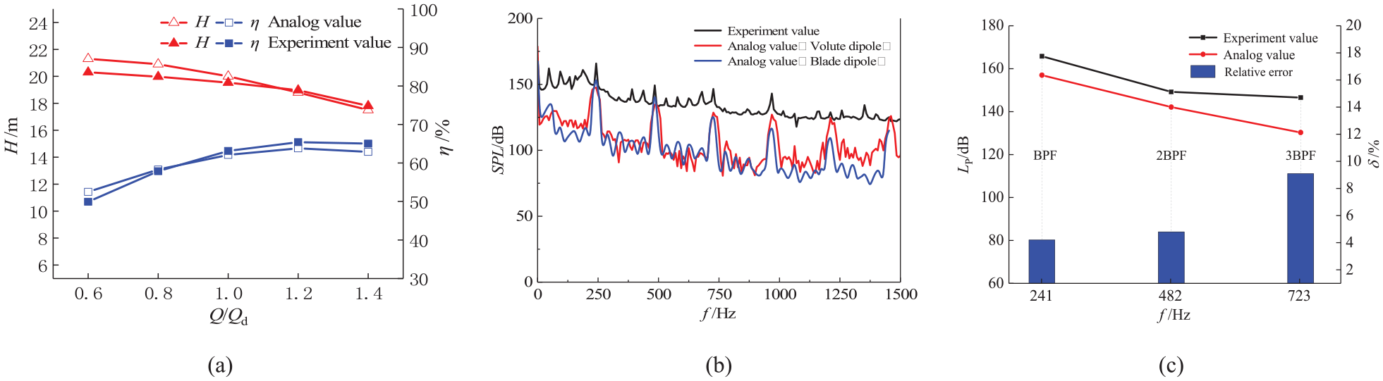
Comparison between numerical calculation and experimental result: (a) hydraulic performance curve, (b) sound pressure level frequency response curve, and (c) noise after stacking.

Figure 7(b) compares the frequency response curve of the outlet sound pressure level obtained from the calculation and test of the internal field noise of the centrifugal pump. In calculating the internal field noise of the centrifugal pump, the rotating blade dipole noise and the static volute dipole noise are calculated to verify the effectiveness of the noise calculation method. The calculated values of the two sound sources within 1500 Hz are lower than the measured values. At the blade passing frequency and its octave, the calculated values of the noise are close to the measured values, which is consistent with the law obtained by Liu et al.¹⁸

The relative error increases with the increase in frequency. The primary reason for this phenomenon is that the influence of pipe resonance, motor operation, cavitation, and backflow inside the pump has not been considered in calculating field noise inside the centrifugal pump. As depicted in Figure 7(b), the peak level of the blade rotating dipole noise is more consistent with the test value only at the blade passing frequency and twice the blade passing frequency.

In contrast, the peak level of the volute stationary dipole noise is more consistent with the test value at more than twice the blade passing frequency. Therefore, the internal field noise of two types of sound sources is superimposed on the corresponding frequency, and the superposition result is expressed by the total sound pressure level L_p, to improve the reliability of noise numerical calculation. The superposition formula is defined in equation (2).

L_{p} = 101 g \sum_{i = 1}^{n} 10^{0.1 L_{Pi}}

(2)

Figure 7(c) compares the noise superposition value of two types of sound sources and the test value. The trend of the two curves is the same, and the maximum sound pressure level appears at the blade passing frequency, at which time the relative error is 4.1%. The maximum relative error in the entire frequency range is 9.6%, satisfying the test error requirements. The comparison result confirms that the noise calculation method adopted can accurately reflect the noise level of centrifugal pumps.

Optimized design

Establishment of optimization parameters and sample space

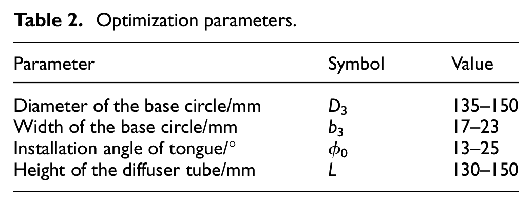
With many types of structural parameters of the centrifugal pump’s volute, each parameter has different effects on performance—some parameters only have significant effects on specific performance. In this study, the relevant parameters are total sound pressure level (L_p) and efficiency (η). As an optimization goal, given the controllability of structural parameters in the spiral case modeling process and the existing conclusions in the reference literature,¹⁹ the influence parameters and intervals of the spiral case structure are selected, as presented in Table 2.

Table 2.

Optimization parameters.

Parameter	Symbol	Value
Diameter of the base circle/mm	D ₃	135–150
Width of the base circle/mm	b ₃	17–23
Installation angle of tongue/°	ϕ₀	13–25
Height of the diffuser tube/mm	L	130–150

The selection of sample points is directly related to the construction accuracy of the approximate centrifugal pump model. Too many sample points will lead to an increase in workload and consumption of computing resources. As a standard test sampling design method,²⁰ the LHS can fully reflect the essential characteristics of the sample space with fewer sampling times, which belongs to stratified sampling technology. The number of samples for training the RBF neural network should follow the n × 10 Principle. The number of samples should be 10 times greater than the independent variable parameters of the input layer. Four volute structure parameters were selected in this optimization process, and the number of sample points was determined to be 41. Its distribution in the sample space is depicted in Figure 8, where the height of the volute diffuser tube L is distinguished by the color bar.

Figure 8.

Sample space distribution.

The 41 samples generated by the LHS are used for numerical simulation calculation, and the results are presented in Table 3. The blade rotating dipole noise (L_p₁) and volute static dipole noise (L_p₂) are calculated for a more accurate noise calculation. The total sound pressure level (L_p) is obtained by noise superposition as defined in equation (2).

Table 3.

Sample data and numerical calculation results.

No.	D ₃/mm	B ₃/mm	ϕ₀/(°)	L/mm	η/%	L_p/dB
1	145	20.2	23.1	139	63.7	154.4
2	149	18.7	20.4	143	62.9	154.2
3	144	18.3	18.1	148.3	63.8	155.1
4	135	18.9	20.7	132.5	64.2	152.8
5	147	22.0	14.2	137.7	61.3	148.8
6	137	21.6	23.4	141.4	63.6	151.2
7	137	22.5	22.4	132.3	63.7	152.3
8	139	21.9	15.1	140.7	63.2	151.4
9	149	18.6	15.8	146.2	62.4	147.9
10	144	20.7	14.1	147.3	62.8	148.9
11	137	22.8	19.7	148.0	63.5	151.6
12	139	20.5	16.0	146.0	63.8	150.9
13	138	20.1	20.9	149.9	64.0	148.0
14	143	19.2	21.9	142.3	63.9	149.7
15	142	17.3	15.4	131.9	61.8	150.1
16	138	17.9	23.6	139.1	64.1	150.1
17	138	17.0	18.9	138.2	64.4	152.4
18	147	18.4	21.7	133.1	62.8	148.2
19	141	22.9	16.6	143.8	63.5	150.6
20	141	17.7	13.8	135.1	61.9	150.2
21	142	19.9	17.2	143.0	63.7	150.1
22	136	19.3	24.8	148.7	63.7	152.3
23	149	20.0	22.3	135.5	62.7	152.6
24	143	19.6	17.0	134.1	63.3	149.7
25	147	17.8	13.5	136.0	61.5	147.6
26	148	21.0	21.5	136.5	63.0	147.8
27	140	17.3	22.8	131.2	64.1	150.2
28	148	21.4	14.6	138.6	60.1	148.0
29	144	22.7	23.9	137.0	63.5	149.5
30	145	20.9	18.3	144.9	63.2	154.9
31	140	22.4	18.6	134.5	63.2	142.9
32	149	19.0	20.0	140.1	62.2	153.0
33	140	18.1	17.5	146.7	64.0	151.2
34	136	19.5	16.4	142.0	64.0	152.6
35	146	22.2	13.3	130.4	57.5	149.1
36	145	21.4	24.6	133.7	63.5	148.5
37	136	17.5	20.0	149.2	64.3	152.4
38	146	19.7	19.4	144.5	63.4	148.0
39	141	21.7	14.9	140.9	63.3	150.3
40	143	20.6	24.3	145.5	63.5	150.2
41	150	21.2	17.8	130.5	61.4	147.2

Construction of RBF neural network agent model

The relationship between the hydraulic and acoustic performance of the centrifugal pump and the structural parameters of the volute is unknown and complex, and the traditional mathematical model has difficulty achieving dynamic expression. The RBF neural network is a feedforward neural network with a three-layer network structure: an input layer, a hidden layer, and an output layer.¹² The formal transformation of sample data from the input layer to the hidden layer is nonlinear, while the transformation from the hidden layer to the output layer is linear.

Figure 9 illustrates the structure of the RBF neural network, where x is the n-dimensional input vector, and c_i is the center of the hidden layer node. q_i is the output of the ith hidden layer node, ϕ_i(*) is the RBF function, ||*|| is Euclidean norm, w_kj is vector output direction, Σ is the linear weighted sum of the outputs of hidden cells, and y is the output vector.

Figure 9.

Schematic of RBF neural network structure.

This study establishes the RBF neural network using the newrb function in MATLAB software. There are four input layer nodes and two output layer nodes. All 41 samples generated by the LHS method participate in the training of the RBF neural network. Under the premise of fully guaranteeing the approximation ability and generalization ability of the constructed RBF neural network, the maximum number of hidden layer neuron nodes is set to 40, the number of iterations is the same as the number of samples, and the target error is 10⁻⁴. The error change curve in the training process is depicted in Figure 10. When the number of iterations reaches 33, the RBF neural network training error is less than the target error, and the training is completed.

Figure 10.

Training error curve of RBF neural network.

Five groups of test data are randomly generated by the LHS method to test the prediction effect of the RBF neural network, as presented in Table 4. The predicted value of the RBF neural network is compared with the calculated value of the CFX, as depicted in Figure 11. In contrast, Figure 11(a) illustrates the comparison results of centrifugal pump efficiency, and Figure 11(b) illustrates the comparison of the total sound pressure level of the centrifugal pump. The maximum error of efficiency is 2.05%, and the maximum error of total sound pressure level is 0.63%, both of which are within the allowable range of test error. Therefore, the trained RBF neural network can accurately predict the efficiency and total sound pressure level within the selected range of volute structure parameters of the centrifugal pump.

Table 4.

Test sample data.

No.	D ₃/mm	b ₃/mm	ϕ₀/°	L/mm
1	138.56	22.88	17.42	149.43
2	135.28	20.27	20.27	140.31
3	149.62	21.14	22.70	134.34
4	141.26	18.25	19.04	130.83
5	145.10	17.04	13.48	142.16

Figure 11.

Comparison between RBF neural network prediction and CFX calculation results: (a) efficiency comparison and (b) comparison of total sound pressure level.

Global optimization based on GA

GA is a computing model based on natural selection and genetic mechanisms. It was first proposed by John Holland in 1975 and has been widely used in machine learning and optimization design research since its introduction in.²¹ In multi-objective optimization design, using GA to find the optimal solution can avoid the complex mathematical solution process. It must produce only the corresponding objective function and fitness function and modify the probability of the optimization population through genetic operators selection, crossover, and mutation to obtain the optimal solution to the problem. The specific process is depicted in Figure 12.

Figure 12.

GA flow chart.

In combination with this research content, GA is used in MATLAB to solve the RBF neural network proxy model constructed to obtain the Pareto optimal solution set of the two objective functions of maximum efficiency of centrifugal pump and minimum total sound pressure level.²² In the specific implementation process, the population fitness evaluation process is provided by the trained RBF neural network. The individual coding process uses actual encoding. The population size is set to 200, the Pareto front-end coefficient to 0.5, the crossover rate to 0.3, and the mutation rate to 0.2.

Results and discussion

Optimization results

After iteration, the Pareto optimal frontier curves for the synergistic optimization of the centrifugal pump efficiency (η) and the total sound pressure level (L_p) were obtained, as depicted in Figure 13. The curve development is relatively smooth, indicating that the Pareto solution set is uniformly distributed. The high optimization performance is similar to the Pareto optimal frontier curve obtained by Shim et al.¹⁹ Table 5 presents the structural parameters and performance of the two extreme individuals of the Pareto solution set compared with the initial individual.

Figure 13.

Pareto optimal frontier curve.

Table 5.

Comparison of structure parameters and performance before and after optimization.

Model	D ₃/mm	b ₃/mm	ϕ₀/(°)	L/mm	η/%	L_p/dB
Initial	140	18	14	140	63.1	152.1
Optimal efficiency	136	17.5	20	148.2	67.2	149.5
Optimum total SPL	142	22.4	18.6	136.5	64.3	142.1

Comparing the two optimized extreme individuals with the initial one, D₃ and b₃ of the optimal efficiency individual have decreased, while ϕ₀ and L have increased. D₃, b₃, and ϕ₀ of the optimal total sound pressure level individual increased, while L decreased. Figure 14 illustrates the changes in the worm shell geometry before and after optimization.

Figure 14.

Geometric structure of spiral case before and after optimization.

Comparison and analysis of hydraulic performance before and after optimization

The two optimized extremal individuals are modeled, numerically calculated, and compared with the initial individuals.

Figure 15 is a comparison chart of hydraulic performance curves. From the perspective of the working conditions of the entire flow point, the trend of the head and efficiency curves after optimization is the same as before optimization. The head curve distribution of the individual with the best efficiency is lower than that of the initial individual at 0.6Q_d, and the curve distribution of other flow points is higher than that of the initial individual. The head curve distribution of the optimal individual of total sound pressure level is the same as that of the initial individual, and the efficiency curve is slightly higher than that of the initial individual when it is more significant than 0.8Q_d. Under rated flow conditions, the head of the best efficiency individual increased by 1.79%, and the efficiency increased by 3.79% compared with the initial individual. The head of the best individual of total sound pressure level does not noticeably change, and the efficiency increases by 1.1%.

Figure 15.

Hydraulic performance curve of centrifugal pump.

The strength of turbulent eddy dissipation can closely reflect the hydraulic performance level of the centrifugal pump. Figure 16 illustrates the distribution of turbulent eddy dissipation in the centrifugal pump’s impeller middle span under rated conditions. The turbulent eddy dissipation in the areas such as the impeller inlet, the interface between the impeller outlet and the volute, and close to the inner wall of the volute is relatively severe, indicating that the flow in these areas has certain instability, and the energy loss is relatively severe. The position of turbulent vortex dissipation is the same before and after optimization.

Figure 16.

Turbulent eddy dissipation distribution in the middle span of centrifugal pump under rated operating conditions: (a) initial individual, (b) efficiency optimal individual, and (c) optimum total sound pressure level.

The turbulent eddy dissipation at the impeller inlet and the interface between the impeller outlet and the volute do not change noticeably. The turbulent eddy dissipation near the inner wall of the volute and the volute diffuser tube is significantly weaker than that of the initial individual, in which the best efficiency individual is the most obvious, followed by the best total sound pressure level individual. These results confirm that the energy loss in the optimized individual is smaller than in the initial individual.

As depicted in Figure 15, the head and efficiency of the optimized individual are significantly improved in the rated working condition and under extensive flow conditions. This finding indicates that the optimized individual has widened the high-efficiency area of centrifugal pump operation to a certain extent. Figure 17 illustrates the streamlined distribution of the middle span of the volute under high flow conditions. Before optimization, the streamline in the volute diffuser is distributed predominantly on both sides of the pipe wall. After optimization, the streamline in the volute diffuser tube is evenly distributed, the flow rate is lower than the initial individual, and the energy loss is slight. The optimal efficiency individual performs best, followed by the optimum individual of the total sound pressure level.

Figure 17.

Streamline distribution in the middle span of spiral case: (a) 1.2Q_d and (b) 1.4Q_d.

During the unsteady calculation of the flow field of the centrifugal pump, the pressure pulsation information at the volute tongue was monitored. The specific location of the monitoring point P₀ is depicted in Figure 4. The time-domain information of pressure pulsation obtained from monitoring is converted into frequency-domain information using the Fourier transform, and the transient pressure is dimensionless processed, as defined by equation (3):

C_{p} = \frac{(P - \bar{P})}{0.5 ρ u^{2}}

(3)

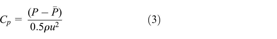
where P is the transient pressure, $\bar{P}$ is the average pressure throughout the cycle, and u is the circumferential velocity at the impeller outlet.

Figure 18 illustrates the spectrum of pressure pulsation monitored at the volute tongue. The peak value of pressure pulsation appears primarily at the shaft frequency, blade passing frequency, and multiple frequencies. The peak value at the blade passing frequency is the largest, and the peak value of pressure pulsation decreases with the increase in frequency. This indicates that the blade passing frequency is the central frequency of pressure pulsation at the volute tongue. Under the three specified working conditions, the peak pressure pulsation of the optimized individual at the blade passing frequency is weakened to varying degrees compared with the initial individual. The rated working condition has the most significant drop, the optimal efficiency individual has a 4.4% drop, and the total sound pressure level optimal individual has a 14% drop.

Figure 18.

Spectrum of pressure fluctuation at volute tongue.

Comparison and analysis of acoustic performance before and after optimization

Based on the flow field calculation of the centrifugal pump, the internal and external sound fields are calculated to explore the changes in acoustic performance of the centrifugal pump before and after optimization.

Figure 19 illustrates the sound pressure level frequency response curves of the internal noise of the centrifugal pump. The development law of sound pressure level frequency response curves for each source term of the three individuals is similar, and the peak values occur primarily at the shaft frequency, blade passing frequency, and octave. The peak values decrease with the increase in frequency. The optimized individual’s sound pressure level frequency response curve is below the initial individual, and the noise reduction effect is significant.

Figure 19.

Centrifugal pump infield-noise sound-pressure-level frequency response curve: (a) volute stationary dipole noise and (b) blade rotating dipole noise.

Table 6 presents the centrifugal pump infield noise’s sound pressure level values at the vane passing frequency for the three specified operating conditions. Under the rated working condition, compared with the initial individual, the total sound pressure level (L_p) of the optimal efficiency individual decreases by 1.4%, and the total sound pressure level (L_p) of the optimum individual of the total sound pressure level decreases by 5.5%.

Table 6.

Noise sound pressure level of the centrifugal pump at blade frequency under various working conditions.

Operating mode	Volute type	Volute dipole	Blade dipole	L_p
0.8Q_d	Initial/dB	144.45	150.17	151.13
	Optimal efficiency/dB	144.36	149.81	150.91
	Optimum total SPL/dB	142.23	148.07	149.12
1.0Q_d	Initial/dB	144.87	149.96	151.23
	Optimal efficiency/dB	143.68	147.64	149.11
	Optimum total SPL/dB	137.89	141.01	142.81
1.2Q_d	Initial/dB	145.36	152.24	152.84
	Optimal efficiency/dB	144.83	149.06	150.31
	Optimum total SPL/dB	142.86	148.37	149.47

Figure 20 illustrates the frequency response curve of the sound pressure level monitored at point M during the calculation of the external noise of the centrifugal pump. Under the three specified working conditions, the trend of each curve is similar. The peak value occurs primarily at the blade passing frequency and its octave. The peak value level gradually decreases with the increase of frequency, among which the peak value level is the highest at the blade passing frequency. The external noise radiation level under extensive flow conditions is higher than in other conditions. Compared with the initial individual, the noise radiation level of the optimized individual decreased in three specified working conditions, of which the effect is most evident in the rated working condition. At the blade passing frequency, the efficiency optimal individual decreases by 0.6%, and the sound pressure level optimal individual decreases by 2.3%.

Figure 20.

Frequency response curve of sound pressure level of external noise of the centrifugal pump.

Figure 21 illustrates the directivity distribution at the passing frequency of the external noise blade of the centrifugal pump under the rated working condition. The directivity distribution shape of the external noise of each plane differs, caused primarily by the difference in the pump body structure and the relative sound source position of each plane. In the x-y and y-z planes, the external noise presents a characteristic dipole distribution, while in the x-z plane, it differs. This is primarily because the x-z plane is located on the middle span of the volute, caused by the structure’s asymmetry and the fluid flow instability at the tongue diaphragm. The directional distribution range of the external noise of the optimized individual in each plane is lower than that of the initial individual the optimal individual of total sound pressure level has the best effect, followed by the optimal individual of efficiency.

Figure 21.

Directional distribution of external noise at the passing frequency of centrifugal pump blade: (a) x-y plane, (b) x-z plane, and (c) y-z plane.

Conclusion

In this study, an RBF neural network and GA are combined to optimize the volute to improve the hydraulic and acoustic performance of the centrifugal pump. The following conclusions are drawn:

(1) The multi-objective optimization method combining RBF neural network and GA achieves the collaborative optimization of the hydraulic and acoustic performance of centrifugal pumps. The (D₃) and (b₃) of the optimal efficiency individual decreased compared with the initial individual, while (ϕ₀) and (L) increased. The (D₃), (b₃), and (ϕ₀) of the optimum individual of total sound pressure level increased compared with the initial individual, while (L) decreased.

(2) The centrifugal pumps’ hydraulic and acoustic performance before and after optimization under different working conditions are compared and analyzed. The results confirm that under different working conditions, the hydraulic and acoustic performance of the optimized individual increases to varying degrees. Under rated conditions, compared with the initial individual, the efficiency of the optimal individual increases by 3.79%, the head increased by 1.79%, the peak value of pressure pulsation at the blade passing frequency decreases by 4.4%, the internal noise decreases by 1.4%, and the external noise decreases by 0.6%. The efficiency of the best individual of sound pressure level increased by 1.1%, the head does not noticeably change, the peak value of pressure pulsation at the blade passing frequency decreased by 14%, the internal noise decreased by 5.5%, and the external noise decreased by 2.3%.

(3) The multi-objective optimization design method adopted in this study applies to the optimization design of the volute of the centrifugal pump. However, whether this method can realize the simultaneous optimization of the impeller and volute requires further study.

Footnotes

Appendix I

Handling Editor: Chenhui Liang

Declaration of conflicting interests

The author(s) declared no potential conflicts of interest with respect to the research, authorship, and/or publication of this article.

Funding

The author(s) disclosed receipt of the following financial support for the research, authorship, and/or publication of this article: This study was financially supported by the National Natural Science Foundation of China (No. 52009050), the Gansu Provincial Natural Science Foundation of China (No. 20JR10RA172), and the Postdoctoral Science Foundation of China (No.2020M673537).

ORCID iD

Rong Guo

References

Zakeri

Paulavets

Barreto-Gomez

, et al. Pandemic, war, and global energy transitions. Energies 2022; 15: 6114.

Gangipamula

Ranjan

Patil

. Flow-induced noise sources and reduction methods in centrifugal pumps: a literature review. Phys Fluids 2022; 34: 081302.

Guo

Zhang

, et al. Influence of blade profile on the hydraulic and rotating noise characteristics of a jet centrifugal pump. Shock Vib 2019; 38: 223–230.

Yang

Ran

, et al. Multi-objective parameter optimization of turbine impeller based on RBF neural network and NSGA-II genetic algorithm. Energy Rep 2021; 7: 584–593.

Zhang

Yang

Zhao

, et al. Optimization design of vane diffuser and volute in vertical centrifugal pump based on back propagation neural network. J Trans Chin Soc Agric Mach 2022; 53: 130–139.

Chen

Xin

Zuguang

, et al. Multi-objective optimization of multistage pump balance drum system based on bp neural network and genetic algorithm. Int J Fluid Machinery Syst 2021; 14: 80–94.

Ren

, et al. Multi-objective optimization on diffuser of multistage centrifugal pump base on ANN-GA. Struct Multidiscipl Optim 2022; 65: 182.

Kim

Ovgor

Cha

, et al. Optimization of the aerodynamic and aeroacoustic performance of an axial-flow fan. AIAA J 2014; 52: 2032–2044.

Lin

Yuan

, et al. Multi-objective optimization on hydraulic design of non-overload centrifugal pumps with high efficiency and low noise. J Trans Chin Soc Agric Eng 2016; 32: 69–77.

10.

Zhao

Xia

Sheng

, et al. Multi-objective parameters optimization of low specific speed centrifugal pump based on NSGA-II genetic algorithm. J Lanzhou Univ Technol 2020; 46: 55–61.

11.

Zhang

Davila

Zangeneh

. Multi-objective optimization of a high specific speed centrifugal volute pump using three-dimensional inverse design coupled with computational fluid dynamics simulations. J Fluid Eng 2021; 143: 021202.

12.

Zhang

. Comparison and research of BP and RBF neural networks in function approximation. Ind Control Comput 2018; 31: 119–120.

13.

Yuan

Wei

, et al. Optimization design of energy-saving mixed flow pump based on MIGA-RBF algorithm. Machines 2021; 9: 365.

14.

Wang

Zhang

. Optimal design of centrifugal pump based on RBF neural network and genetic algorithm. J China Three Gorges Univ Nat Sci 2020; 42: 88–93.

15.

Wang

Han

Pei

, et al. Energy efficiency optimization of water pump based on heuristic algorithm and CFD. J Comput Des Eng 2022; 10: 382–397.

16.

Wang

Chen

, et al. Internal flow characteristics of high-specific-speed centrifugal pumps with different number of impeller blades under large flow conditions. Machines 2023; 11: 138.

17.

Wang

, et al. Experimental investigation on the water hammer characteristic of stalling fluid in eccentric casing-tubing annulus. Energy 2022; 253: 124113.

18.

Liu

Cheng

, et al. Collaborative improvement of efficiency and noise of bionic vane centrifugal pump based on multi-objective optimization. Adv Mech Eng. Epub ahead of print 14 February 2021. DOI: 10.1177/1687814021994976.

19.

Shim

Kim

. Design optimization of the impeller and volute of a centrifugal pump to improve the hydraulic performance and flow stability. J Fluid Eng 2020; 142: 101211.

20.

Zheng

Liu

Song

, et al. Preliminary study on improved Latin hypercube sampling. Nucl Electron Detect Technol 2017; 37: 734–738.

21.

Jiang

Yang

Bai

, et al. Optimization of centrifugal pump blade based on high-dimensional hybrid model and genetic algorithm. J Huazhong Univ Sci Technol Nat Sci Ed 2020; 48: 128–132.

22.

Zhao

Pei

Yuan

, et al. Energy-saving oriented optimization design of the impeller and volute of a multi-stage double-suction centrifugal pump using artificial neural network. Eng Appl Comput Fluid Mech 2022; 16: 1974–2001.

Multi-objective optimization design in a centrifugal pump volute based on an RBF neural network and genetic algorithm

Abstract

Keywords

Introduction

Numerical computation

Basic parameters of the model

Grid generation and boundary condition setting

Computational model validation

Optimized design

Establishment of optimization parameters and sample space

Construction of RBF neural network agent model

Global optimization based on GA

Results and discussion

Optimization results

Comparison and analysis of hydraulic performance before and after optimization

Comparison and analysis of acoustic performance before and after optimization

Conclusion

Footnotes

Appendix I

Declaration of conflicting interests

Funding

ORCID iD

References