Sage Journals: Discover world-class research

Abstract

The complex curved boundary of the topology optimization model is not conducive to industrial manufacturing hence the necessity to reconstruct the geometrical model. This study presents a general method for the boundary regularization fitting reconstruction of a topological optimization model based on the Freeman code. This method is performed as follows: the unit vector is defined; the vectorized expression of the Freeman code boundary is established; through the concept of the boundary bending parameter, determination of the bending degree of the Freeman code boundary is established; an elemental structure analysis method is proposed, and the logic of the automatic extraction of the control points of the Freeman code boundary fitting is achieved. This method proposes a series of innovative technical methods, such as unit vector definition, boundary bending matrix, and elemental structure analysis method, and designs a complete set of structural analysis logic for a Freeman code type boundary, which can automatically analyze the structure feature of the 8-connected Freeman code boundary, extract the fitting control points on the boundary, and complete the automatic fitting and reconstruction of the boundary. This method is robust and applicable to all Freeman code boundaries. The entire process is automated.

Keywords

Topology optimization industrial manufacturing boundary regularization fitting Freeman code automatic fitting

Introduction

Topology optimization technology is widely used in mechanical design. It can rapidly and efficiently calculate the optimal distribution of materials in space and design an optimal structure.^1–3 Then, it provides the conceptual configuration and innovation scheme for mechanical design.

The complex curved boundary of the topology optimization model is not conducive for traditional manufacturing. It is necessary to fit the complex curved boundary into a smooth, regular boundary form without change the structural skeleton feature. This process is called regularization reconstruction of the topological optimization structure. The traditional method is to manually redraw the geometric model using CAD software. This model reconstruction method significantly affects the overall design efficiency and is influenced by human factors. This is an important practical problem for topology optimization design and application to efficiently convert the topology optimization model into a parametric geometric model.

Based on this problem, considerable research has been conducted. Bendsøe and Sigmund⁴ initially integrated image-processing technology into the boundary extraction of the topology structure. Christiansen et al.⁵ proposed an optimization method based on deformable geometry. It combines topology and shape optimization of 3D structures. Garrido-Jurado et al.⁶ and Tompson et al.⁷ researched computer image recognition. Guo et al.⁸ adopted level set^9,10 functions to describe the topological results based on rectangular geometric feature. Recently, van Dijk et al.¹¹ conducted a preliminary study on the boundary extraction of a two-dimensional (2D) topological structure based on image processing technology. Yi and Kim¹² studied a processing method for small feature in the topological boundary of the SIMP method and perfected the boundary extraction technology of the 2D topological structure.

As the most commonly used function model in the field of computer image processing, the non-uniform rational basis spline (NURBS) is widely used in the research of complex surfaces.^13–18 The density based on an algorithm based on NURBS surfaces and hypersurfaces in Costa et al.¹⁹ and Rodriguez et al.²⁰ provides CAD-compatible entities at the end of the optimization process without any post-processing stage in the CAD software. Giulia²¹ proposed a meta-modeling strategy based on the NURBS hypersurface, which realizes the parametric fitting reconstruction of complex surfaces by defining the number, position, weight, control parameters, and other factors of control points.

In contrast to previous research methods, the object of this method was the Freeman code boundary. The Freeman code method is often used to express planar curves and closed regions.²² Compared to other boundary expression methods, the Freeman code method completes the boundary digital expression by coding the boundary pixels.²³ This coding method is insensitive to rotation, translation, scaling, and other operations. It can express the boundary attributes of a target in a more stable manner. In addition, the boundary points expressed by the freeman code method have strong regularity in spatial arrangement, and it expresses complex irregular curves as freeman code boundaries.^24,25

The research content of this study includes three innovative technical methods: 1. The concept of a unit vector is proposed based on the Freeman code boundary. A set of standardized analysis methods based on the Freeman code boundary is created. The unit vector is used to vectorize the expression of the Freeman code boundary. This expression method can describe the structural shape of all Freeman code boundaries and has strong universality; 2. Based on the vectorization expression of the Freeman code boundary, the concept of boundary bending matrix is proposed. A bending matrix is used to calculate the bending degree of the Freeman code boundary; 3. An elemental structure analysis method was proposed to analyze and extract the fitting control nodes of the Freeman code boundary.

Compared to other fitting reconstruction methods, the research method has the following two advantages: 1. The algorithm rapidly fits the irregular complex curve boundary into a straight-line boundary to a high-quality, and the entire process is automatically processed; 2. The algorithm is applicable to all 8-connected Freeman code boundaries and exhibits strong robustness. This method completes the automatic conversion from a topology optimization structure to an industrial production manufacturing model.

The remainder of this paper is organized as follows: Section 2 presents the Freeman code technology and the boundary detection method; Section 3 presents the mathematical expression of the Freeman code boundary, and proposes the elemental structure analysis method; Section 4 analyses the classification and structural feature of the Freeman code boundary and completes the engineering straight fitting of the boundary. In Section 5, the decision strategy of the control points on the regularization fitting boundary is introduced and the boundary is rounded. The judgment logic of the control points on the fitting boundary and the fillet processing of the boundary are described; Section 6 presents a general analysis of the method; Section 7 summarizes the study and presents the scope for future research.

Expression of the boundary in Freeman code form

In this section, all boundaries of the topology optimization model are quantified by the Freeman code method to describe the attributes of the objective boundary, thus established the digital expression of the boundaries of the topology optimization model.

Principle of the Freeman code

The Freeman code method detects the outermost nonzero boundary points of the objective (including the inner hole boundary) in the binary image and expresses the boundary contour of the target in the form of a Freeman code.

The principle of the Freeman code method is to search the position of the next boundary point clockwise in its neighborhood, with the center as the starting pixel, traverse all boundary points on the boundary in turn, and stop the calculation at the end pixel of the boundary. Subsequently, the direction codes of all the boundary points are recorded in a matrix to form a point set, thereby completing the expression of the objective boundary.

Freeman codes are divided into 4- and 8-connected codes according to the neighborhood connection number of the boundary pixel points, as shown in Figure 1. Compared with the 4-connected Freeman code, the 8-connected Freeman code adds four oblique directions which correspond to the actual pixel arrangement. The 8-connected freeman code can express the boundary of the objective more accurately.

Figure 1.

Freeman code: (a) 4-connected and (b) 8-connected.

Freeman code expression for objective boundary

Noise exists in the original model and affects boundary recognition. The binary method converts the multi value digital image to the binary image to express the model boundary more clearly. Figure 2 shows image binarization of the topology-optimized cantilever structure.

Figure 2.

Image binarization of cantilever beam.

The inner function bwboundaries on MATLAB were used to extract the contour of the binary image, and the boundary point information was stored in the cell array. The boundary detection is based on Freeman code technology, which automatically tracks and extracts the contour of the outer and inner boundaries in the binary image. The extracted boundary points are represented by 8-connected Freeman codes to realize the vectorization output of the boundary of the topology optimization model.

As shown in Figure 3, the vectorized boundary model of the cantilever beam structure is composed of multiple connected domains. The red point in the figure is the coordinate origin and the boundary point closest to the origin in each connected domain is the boundary starting point.

Figure 3.

8-connected Freeman code boundary of the initial model.

Analyzing the structural feature of Freeman codes boundary

The structural feature of Freeman code boundary is analyzed to provide a theoretical basis for the extraction of boundary control points. This section is divided into three steps: (a) Vectorization expression of the Freeman code boundary; (b) Determination of bending degree of Freeman code boundary; (c) Detection of boundary structure feature of Freeman codes.

Vector expression of Freeman code boundary

In this section, the concept of unit vector is proposed to transform the boundary feature analysis problem into the unit vector arrangement problem, thus realize the vectorization expression of Freeman code boundary.

Figure 4(a) shows an 8-connected Freeman code, with fixed connection positions of the neighboring pixels. The vector is a quantity that describes the direction and length. Through the concept of vectors, the connection form of the 8-connected Freeman code can be converted into a vector form. The coordinates of the central pixel point of the Freeman code are defined as (0,0), and the coordinates of the 8-pixel points in the neighborhood are shown in Figure 4(a). The central pixel of the Freeman code was sequentially connected to eight neighboring pixel points to obtain eight vectors. The lengths and directions of the eight vectors were fixed. 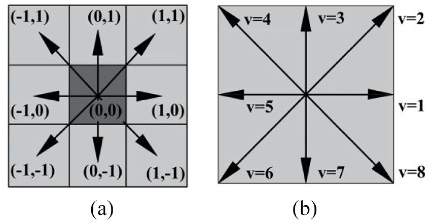They are called the unit vectors of the 8-connected Freeman code boundary and are represented by the letter v. Each unit vector corresponds to a number from 1 to 8, as shown in Figure 4(b). The length of the four odd vectors in the right-angled direction was 1, and the length of the four even vectors in the oblique direction was $\sqrt{2}$ . The corresponding relationships between the lengths of unit vectors v are listed in Table 1.

Figure 4.

Coordinates of neighborhood boundary points of 8-connected Freeman codes: (a) coordinate of freeman code and (b) Unit vector of freeman code.

Table 1.

Corresponding parameters of the unit vectors.

Unit vector	→	↗	↑	↖	←	↙	↓	↘
v	1	2	3	4	5	6	7	8
Coordinate	(1,0)	(1,1)	(0,1)	(−1,1)	(−1,0)	(−1, −1)	(0, −1)	(1, −1)
Length	1	$\sqrt{2}$	1	$\sqrt{2}$	1	$\sqrt{2}$	1	$\sqrt{2}$
Direction	0	π/4	π/2	3π/4	π	5π/4	3π/2	7π/4

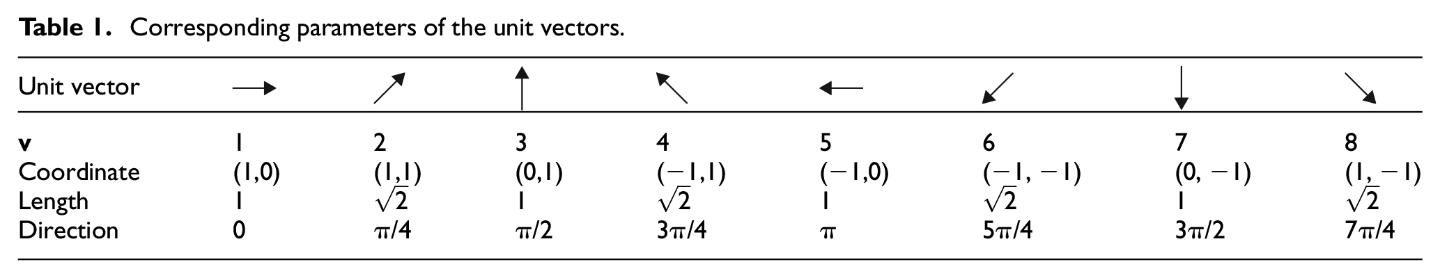
For the 8-connected Freeman code boundary, the coordinate difference between the adjacent boundary points on the boundary is calculated in sequence from the starting point, as shown in equation (1). The coordinate difference information corresponds to the coordinates of the unit vectors in Table 1 to obtain the unit vector v constituting the Freeman code boundary.

(Δ x_{i}, Δ y_{i}) = (x_{i + 1} - x_{i}, y_{i + 1} - y_{i})

(1)

where Δx and Δy represent the differences between horizontal and vertical coordinates, respectively. x and y are the horizontal and vertical coordinates of the boundary point, respectively. i denotes the corresponding boundary point.

The arrangement form of the unit vector constituting the Freeman code boundary is calculated using equation (1), thereby realizing a vectorized expression of the Freeman code boundary. The vector matrix expressing the Freeman code boundary is called the vector expression of the Freeman code boundary, and is expressed by the letter L, as shown in equation (2).

L = [v_{1} v_{2} \cdot \cdot \cdot v_{n}]

(2)

In equation (2), v and n represent the unit vector and number of boundary points, respectively.

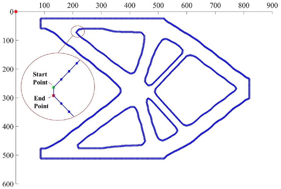
Vector expression L digitizes the structural feature of the Freeman code boundary, and contains the information of each unit vector.

For the Freeman code boundaries shown in Figure 5, and the red dot represents the starting point of the boundary. The vector expression of this boundary is L = [1 8 1 3 4 3 5 7 5 7].

Figure 5.

Freeman code boundary and corresponding unit vector v.

Figure 6 shows the vector expression of the Freeman code boundary of the cantilever beam. The green boundary point in the figure represents the starting point of one of the boundaries, and the red point represents the endpoint of the boundary.

Figure 6.

Cantilever beam freeman code boundary points and corresponding unit vectors.

Determination of bending degree of Freeman code boundary

The degree of bending is the basic structural feature of the boundary. This section describes the detection and calculation method of the bending degree of the Freeman code boundary through the concept of the unit boundary bending parameter.

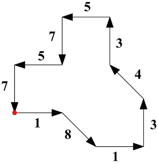
As shown in Figure 7, The boundary expressions were L_a = [1 2 3 4 5], L_b = [1 1 1 1], and L_c = [1 8 7 6 5]. The degree of change of the unit vector reflects the bending degree of the boundary. Equation (3) determines the difference between adjacent unit vectors on the boundary, which is called the boundary bending parameter, and is expressed by the letter P.

P_{i} = (v_{i} - v_{i - 1})

(3)

Figure 7.

Freeman code boundaries: (a) boundary a, (b) boundary b, and (c) boundary c.

Where P, v, and subscript i represent the boundary bending parameter, unit vectors of the boundary, and corresponding boundary point, respectively.

The bending parameter P on the boundary is arranged to form a new matrix, which is called the boundary bending matrix and is represented by the letter P, as shown in equation (4).

P = [P_{2} P_{3} \cdot \cdot \cdot P_{n - 1}]

(4)

Where P, P, and subscript n represent the boundary bending parameter, boundary bending matrix, and corresponding unit vector of the boundary, respectively.

The boundary bending matrices of boundaries L_a and L_b were calculated using equation (4) as P_a = [1 1 1 1] and P_b = [0 0 0]. The boundary bending parameter P at each point on the L_a boundary was 1, indicating that the bending degree of the boundary changed uniformly. The boundary bending parameter P at each point in L_b was 0, indicating that the boundary is a straight line.

In Figure 7, it appears that the boundaries L_a and L_c have the same bending degree and different bending directions; however, using equation (4) results in P_c = [7 −1 −1 −1] which has no correlation with P_a. Therefore, equation (4) requires further modification.

As shown in Figure 8(a), the unit vector changes in an anti-clockwise direction. The letters C and A indicate clockwise and anti-clockwise, respectively. As shown in Figure 8(b), when the unit vector changes from v₁ to v₂, the bending parameter p has two expressions: anti-clockwise and clockwise. When the unit structure changes anti-clockwise, the bending parameter is determined to be P_A= v₂−v₁; When the unit vector changes clockwise, the bending parameter is determined to be P_C = 8-(v₂−v₁). To distinguish bending parameters in two directions, the anti-clockwise change parameter P_A has a plus sign and the clockwise change parameter P_C has a minus sign, so the expression of P_C is (v₂−v₁)−8. The relationship between P_A and P_C is given by equation (5).

P_{A} - P_{C} = 8

(5)

Figure 8.

Change direction of unit vector: (a) unit vector and (b) two change directions.

Table 2 shows the corresponding relationship between the clockwise bending parameter P_C and the anti-clockwise bending parameter P_A.

Table 2.

Corresponding relationship of boundary bending parameter P.

Anti-clockwise (P_A)	7	6	5	4	3	2	1	0
Clockwise (P_C)	−1	−2	−3	−4	−5	−6	−7	−8

According to equation (5), all bending parameters P can be converted into the form of |P| ≤ 4. This process is called normalization of bending matrix. The normalization method of boundary bending matrix can achieve the accurate judgment of boundary bending degree and direction.

The normalization method changes the bending matrix of L_c boundary from P_c = [7 −1 −1 −1] to P_c = [−1 −1 −1 −1]. Compared with P_a, the absolute value of the bending matrix of the two boundaries is the same, indicating that the bending degree of the two boundaries is the same; The starting unit matrix of the two boundaries is v₁= 1, and the symbols of the elements in P_a and P_c are opposite, indicating that the bending directions of the two boundaries are completely opposite.

The bending matrix P of the boundary can accurately describe the bending degree and direction of the Freeman code boundary through mathematical language.

Elemental structure analysis method

Based on the concept of the bending matrix P, this section proposes an elemental structure analysis method to complete the structural shape analysis and boundary control point extraction of all Freeman code boundaries.

Definition of the elemental structure

As shown in Figure 9, the boundary consists of a basic structure. The mathematical expression for the boundary in Figure 9 is L_a = [1 2 1 2 1 2], and the expression for the basic structure is [1 2]. The minimum boundary structure that satisfies the following two conditions is called the boundary element structure.

(1) The elemental structure contains only one or two types of unit vectors.

(2) When the structure contains two types of unit vectors, the first unit vector is not equal to the last vector.

Figure 9.

Freeman code boundary and its element structure.

The above two conditions can be expressed mathematically, as shown in equation (6).

E = [v_{a}] | | [v_{a} v_{b}], v_{a} \neq v_{b}

(6)

where E and v represent the element structure and unit vector of the boundary, respectively. The subscripts represent different unit vectors.

The basic structure shown in Figure 9 meets equation (6), thus it is an elemental structure. The elemental structure is the basic structure of the boundary, and it contains the structural feature of the boundary.

Vector representation of elemental structure

The elemental structure is composed of unit vector. This section will achieve the vectorization of elemental results. First, the slope of a unit vector of the 8-connected Freeman codes were calculated using equation (7), and is denoted by the letter S.

S = \frac{y_{v}}{x_{v}}

(7)

where S represents the slope of the unit vector of the boundary, subscript v is the corresponding unit vector, and x and y respectively represent the horizontal and vertical coordinates of the boundary point corresponding to the unit vector v. The corresponding relationships between the slopes, S, of the 8-connected vectors and coordinates are listed in Table 3.

Table 3.

Coordinates and slope of unit vector.

v	1	2	3	4	5	6	7	8
Coordinates (x, y)	(1,0)	(1,1)	(0,1)	(−1,1)	(−1,0)	(−1, −1)	(0, −1)	(1, −1)
Slope (S)	0	1	∞	−1	0	1	∞	−1

Based on the concept of vector summation, the unit vectors in the element structure are summed and the sum vector is represented by the letter v_E. In Figure 10, the green vector represents the sum vector v_E of the unit vectors. The vector v_E is called the elemental structure vector. The slope of the vector v_E is calculated using equation (8) and is expressed as S_E.

S_{E} = \sum_{i = 1}^{n} y_{i} / \sum_{i = 1}^{n} x_{i}

(8)

Figure 10.

Elemental structure vector.

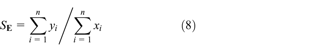
where S_E represents the slope of the elemental structure vector; x and y represent the coordinates corresponding to the unit vector, as shown in Table 3; the subscript i represents the corresponding unit vector in the elemental structure; and n represents the number of unit vectors in the elemental structure.

Equation (8) shows that the elemental structure vector v_E is unique for each element structure. According to the concept of vector summation, the value range of the slope S_E of the unit structure vector is between those of the slope S of the unit vectors.

The elemental structure is used to analyze the structural feature of the Freeman code boundary, and provide a judgment basis for the extraction of boundary control points.

Regularization fitting of the Freeman code boundary

Regularization fitting of basic boundary

As shown in Figure 11, the expression of the elemental structure is E = [1]. The boundary expression is L = [1 1 1 1 1]. This type of boundary, formed by a single unit vector v is called Type I of the basic boundary. The expression for Type I of the basic boundary can be converted to equation (9).

L_{I} = n E, E = [v_{a}]

(9)

Figure 11.

Type I Freeman code boundary.

where L_I, E, and n represents Type I of the basic boundary, elemental structure of the boundary, and number of elemental structures.

Type I of the basic boundary is composed of a single-unit vector, which is a straight-line boundary. It does not require boundary regularization fitting, and there is no control node on the boundary.

Figure 12, this shows a Freeman code boundary. The expression of this boundary is L_II = [1 1 8 1 1 8 1 1 8], and the expression of the elemental structure is E = [1 1 8]. This type of boundary, composed of two types of unit vectors, is called Type II of the basic boundary, and its expression can be expressed as equation (10).

L_{II} = n E, E = [v_{a} v_{b}], v_{a} \neq v_{b}

(10)

Figure 12.

Type II Freeman code boundary.

where L_II, and E represent Type II of the basic boundary and the elemental structure of the boundary, respectively. v_a and v_b represent the unit vectors of Type II. n represent the number of elemental structures.

The vector expression of the elemental structure in the previous section, v_E is substituted into equation (10) to obtain another expression for the boundary, as shown in equation (11).

L_{II} = [v_{E} v_{E} \cdot \cdot \cdot v_{E}]

(11)

where L_II represents Type II of the basic boundary. v_E represent the vector expression of the elemental structure.

The bending degree of Type II of the basic boundary is calculated according to equation (11). The bending matrix P is expressed as shown in equation (12).

P_{II} = [00 \cdot \cdot \cdot 0]

(12)

where P_II represents the bending matrix of Type II of the basic boundary.

The bending parameter P in equation (12) is equal to 0, meeting the definition of straight-line boundary. The regularization fitting results of Type II basic boundary is shown in Figure 13.

Figure 13.

The two types of basic boundary: (a) type I basic boundary and (b) type II basic boundary.

Based on the elemental structures analysis method, this section determines that the basic boundary has the property of a straight-line boundary. The fitting results for these two boundary types are shown in Figure 13.

Regularization fitting of composite boundary

Figure 14 shows the vectorized boundary of the cantilever beam model. This boundary is determined to be composed of three elemental structures by the elemental structure analysis method, and the elemental structure is shown in Figure 14(a). This type of boundary composed of multiple basic boundaries is called a composite boundary, and its expression is shown in equation (13).

L_{C} = \sum_{i = 1}^{n} N_{i} E_{i}

(13)

Figure 14.

Composite boundary in cantilever beam model: (a) composite boundary structure information and (b) boundary regularization fitting results.

where L_C, E respectively represent the composite boundary and elemental structure of the boundary. i and N represent the different elemental structures, and number of each elemental structure, respectively.

The basic boundary can be fitted to a straight-line boundary, but the composite boundary is composed of multiple basic boundaries. Therefore, the fitting control point is located at the intersection of the different elemental structures, as indicated by the red dot in Figure 14(b). Multi-segment line fitting was performed on the composite boundary, and the obtained fitting boundary is shown as the green line segment in Figure 14(b).

All 8-connected Freeman code boundaries can be described as basic or composite boundaries. This method applies to all 8-connected Freeman code boundaries.

Boundary regularization fitting of the topological optimization model

Figure 15(a) shows the Freeman code boundary model for the cantilever case. The boundary control points of the cantilever beam can be extracted using the elemental structures analysis method. The control points are indicated by the red dots in the figure. Subsequently, polyline fitting was performed on the boundary, and the fitting result is shown in Figure 15(b).

Figure 15.

Regularization fitting of cantilever beam boundary: (a) inflection points and (b) fitting reconstruction boundary.

Post-processing of the reconstructed boundary

Post-processing includes three main steps: 1. Controllability of boundary control points; 2. Filleting of the fitting boundary; 3. Simple 3D model reconstruction with regularized boundary.

Controllability of boundary control points

In this section, the controllability method of the control points on the boundary-fitting model is proposed. The boundary control points were filtered by introducing control parameters and setting different values. Control points with low impact on the boundary structure feature were removed, high-quality boundary control points were retained, and the controllability of the control points was realized. This parameter known as the boundary control point parameter is represented by the letter c.

Unnecessary control points increase the salient points of the boundary and affect the quality of the fitting boundar hence the need to eliminate them. Parameter c is a manually set angle. There is no control point with an angle greater than or equal to 180° on the fitting boundary, so the value range of parameter c is less than 180°, as shown in equation (14). Therefore, comparing the angle of all control points on the boundary with the parameter c, if the control point is close to 180°, then the slope of the fitting straight-line boundary on both sides of the control point is closer, which lowers the quality of the control point. Using this method, low-quality control points are detected and deleted, and high-quality control points are retained to realize the controllability of the control points.

c = {x | 0 < x < 180, x \in R}

(14)

By setting different c parameters, the controllability of the control points of the cantilever beam-fitting boundary was achieved. The fitting results are shown in Figure 16(a) and (b) where parameter c was set to 170° and 160°, respectively.

Figure 16.

Boundary fitting model of the cantilever beam with different control points: (a) boundary fitting results at c = 170° and (b) Boundary fitting results at c = 160°.

The two results indicate that when the control parameter c is set closer to 180°, the extraction result of the control points is closer to the original fitting boundary model. This process effectively controls the number of boundary control points, further improves the quality of the fitting boundary, renders the fitting boundary smoother, and is convenient for production.

Fillet processing of fitting boundary

The fitting boundary was composed of straight lines, and there was stress concentration at the control point of the boundary. This section fills the control points of the fitted boundary to ensure that the fitting boundary has good mechanical properties.

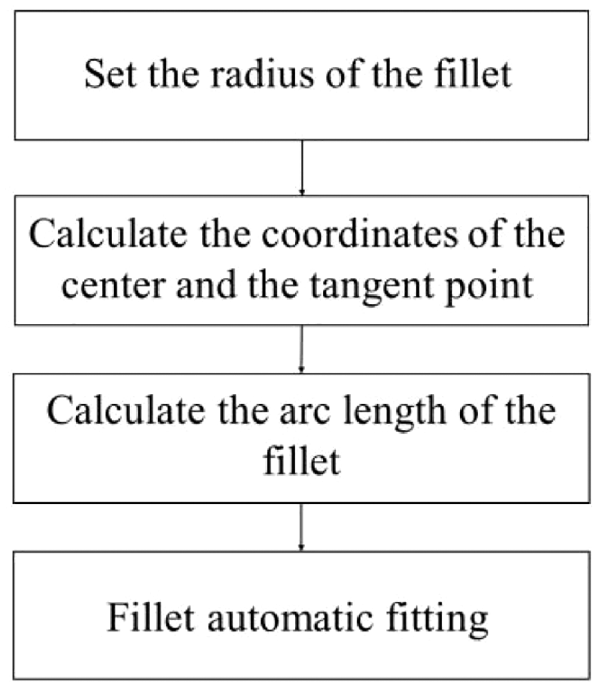
To satisfy different design requirements, a controllable processing method for fillet fitting was proposed. Fillet fitting can be performed by setting different fillet radii to achieve free control.

The entire fillet process of the control points is illustrated in Figure 17. First, radius r was set to meet the design and manufacturing requirements. The algorithm can automatically extract the center of the circle, arc length, and other important parameters to automatically generate the fillet fitting results required by the design, and the entire program is automated.

Figure 17.

Control point fillet fitting process.

Figure 18 shows the final regularization fitting reconstruction model of the cantilever beam, in which the fillet radius r is set to 4 mm.

Figure 18.

Fillet fitting results of cantilever beam control points.

Parametric output of the reconstructed model

The geometric information data of the fitting reconstruction model are stored in MATLAB, and the parametric output of the model was automatically realized through the data conversion interface on MATLAB. As shown in Figure 19, the reconstructed model of the cantilever beam was output to the CAD software, SolidWorks to generate a 2D sketch model.

Figure 19.

Sketch of cantilever beam reconstructed boundary.

In the CAD software, through the operation of extruding feature, the fitting reconstruction model in the sketch is generated into a 3D regularization geometric model. Figure 20 shows the 3D regularization fitting model generated by stretching the regularization boundaries of the cantilever beams.

Figure 20.

3D reconstruction model of the cantilever beam.

Applications and verification

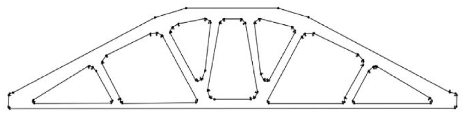
Figure 21 shows the bridge topology optimization structure model. The boundary regularization fitting reconstruction of the structure is completed through the proposed strategy, as shown in Figure 22. First, the boundary model of 8-connected freeman code is extracted by the boundaries method as shown in Figure 22(a). Then, based on the definition of the element structure, the structure of the freeman code boundary is analyzed, and the regularization fitting reconstruction of the Freeman code boundary is completed, as shown in Figure 22(b). Then, the redundant control points on the boundary are filtered out through the control point judgment logic, as shown in Figure 22(c). Finally, through the fillet fitting of boundary control points, the final boundary regularization fitting model is obtained, as shown in Figure 22(d).

Figure 21.

Comparison diagram of the cantilever beam model.

Figure 22.

Cantilever beam model: (a) Freeman code boundary model, (b) regularized fitting boundary model, (c) control point extraction model, and (d) Final regularized reconstruction model.

Subsequently, the regular fitting model of the bridge was imported into the SolidWorks software to generate a 2D sketch model, as shown in Figure 23.

Figure 23.

Parametric sketch model.

The sketch model of the bridge structure was stretched into a 3D regular boundary model by a simple stretching feature operation. The reconstructed model has the same thickness as the original model. The original topological model of the bridge structure was compared with the 3D regular fitting model formed by stretching, as shown in Figure 24.

Figure 24.

Comparison diagram of bridge structure model: (a) original topology model and (b) 3D reconstruction model.

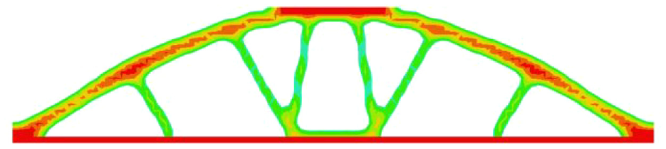
Compared to the original topology optimization model, the surface quality of the 3D regular fitting model was significantly improved. To verify the mechanical properties of the reconstructed model, the original and reconstructed models were simulation experiment using the HyperWorks finite element software. The structural mechanical properties of the two groups of models were compared under the same grid size and load constraints, and the results are shown in Figure 25.

Figure 25.

Stress and displacement nephogram of conceptual bridge structure: (a) original structure stress, (b) original structure displacement, (c) restructure structure stress, and (d) restructure structure displacement.

The results of the analysis are presented in Table 4. Compared with the original structure, the maximum displacement of the concept bridge reconstructed model decreases by 18.2% and the maximum stress decreases by 25.6%.

Table 4.

Reconstructed model and initial structural mechanics performance analysis.

	Maximum stress (MPa)	Maximum displacement (mm)	Volume (mm³)
Original structure	7.842 × 10³	0.800	4530.362
Restructure modle	6.495 × 10³	0.595	4465.788
Comparison	18.2%↓	25.6%↓	1.43%↓

The experimental results show that the reconstructed model has the quality (volume) close to that of the original topology optimization model. The fillet processing of boundary effectively reduces the maximum stress and displacement, and improves the structural performance of the reconstructed model.

Conclusions

In this study, a geometric reconstruction method for a topological optimization model based on the Freeman code boundary is proposed. This method proposes a complete set of structural feature analysis logic for the Freeman code boundary. The mathod can automatically extract the fitting control points of the boundaries, and realize the regularization fitting reconstruction of the boundaries. In addition, the following apply:

The method can automatically analyze and detect complex curve boundaries in topological models. On the premise of not deteriorating mechanical performance, the irregular complex boundary is fitted into the regular straight-line boundary to realize the regular reconstruction of the boundary of the topological optimization model.

The method has strong robustness. It can analyze and detect all 8-connected Freeman code boundaries, and if it is a boundary model expressed by the 8-connected Freeman code, it can realize regular fitting of its boundaries, and the entire process is fully automated.

The boundary regularization fitting reconstruction proposed in this study, which is mainly based on the regularization fitting reconstruction of 2D planar topological boundaries, and formation of a 3D structure model in space through a simple stretching operation. In future research, the team will add simple geometric feature to the fitting boundary, such as regular curves, and add the fitting scheme of the method. Finally, based on the boundary analysis and judgment logic of the 2D plane, the team performed a geometric reconstruction of the complex surfaces in 3D space.

Footnotes

Handling Editor: Chenhui Liang

Declaration of conflicting interests

The author(s) declared no potential conflicts of interest with respect to the research, authorship, and/or publication of this article.

Funding

The author(s) disclosed receipt of the following financial support for the research, authorship, and/or publication of this article: This article acknowledges the support of the Cultivation Program for Young Backbone Teachers at Henan University of Technology (No. 2022Shenhuipeng), Key Technology Research and Development Program of Liaoning Province (No. 2021JH 1/10400099 Research Project 4), Fundamental Research Funds for the Henan Provincial Colleges and Universities in Henan University of Technology (No. 2018QNJH18), and Scientific Research Program of Henan University of Technology (No. 2018BS023).

ORCID iD

Xingchen Wu

References

Zhu

Zhou

Wang

, et al. A review of topology optimization for additive manufacturing: Status and challenges. Chin J Aeronaut 2021; 34: 91–110.

Pedersen

CBW

Allinger

. Industrial implementation and applications of topology optimization and future needs. In: IUTAM symposium on topological design optimization of structures, machines and materials, 2006. pp.229–238. Dordrecht: Springer.

Zhou

Fleury

Patten

, et al. Topology optimization-practical aspects for industrial applications. In: Proceedings of the 9th world congress on structural and multidisciplinary optimization, Shizuoka, Japan, 2011. pp.13–17.

Bendsøe

Sigmund

. Material interpolation schemes in topology optimization. Arch Appl Mech 1999; 69: 635–654.

Christiansen

Bærentzen

Nobel-Jørgensen

, et al. Combined shape and topology optimization of 3D structures. Comput Graph 2015; 46: 25–35.

Garrido-Jurado

Muñoz-Salinas

Madrid-Cuevas

, et al. Automatic generation and detection of highly reliable fiducial markers under occlusion. Pattern Recognit 2014; 47: 2280–2292.

Tompson

Stein

Lecun

, et al. Real-time continuous pose recovery of human hands using convolutional networks. ACM Trans Graph 2014; 33: 1–10.

Guo

Zhang

Zhong

. Doing topology optimization explicitly and geometrically—a new moving morphable components based framework. J Appl Mech 2014; 81: 081009 (12 pages).

Chen

Lee

. Level set based robust shape and topology optimization under random field uncertainties. Struct Multidiscipl Optim 2010; 41: 507–524.

10.

Chen

. A new level-set based approach to shape and topology optimization under geometric uncertainty. Struct Multidiscipl Optim 2011; 44: 1–18.

11.

van Dijk

Maute

Langelaar

, et al. Level-set methods for structural topology optimization: a review. Struct Multidiscipl Optim 2013; 48: 437–472.

12.

Kim

. Identifying boundaries of topology optimization results using basic parametric features. Struct Multidiscipl Optim 2017; 55: 1641–1654.

13.

Bertolino

Montemurro

Perry

, et al. An efficient hybrid optimization strategy for surface reconstruction. Computer Graphics Forum 2021; 40: 215–241.

14.

Liu

, et al. A realization method for transforming a topology optimization design into additive manufacturing structures. Engineering 2018; 4: 277–285.

15.

Cashman

Augsdörfer

Dodgson

, et al. NURBS with extraordinary points: high-degree, non-uniform, rational subdivision schemes. ACM SIGGRAPH 2009 papers, 2009, pp.1–9.

16.

Audoux

Montemurro

Pailhès

. A metamodel based on non-uniform rational basis spline hyper-surfaces for optimisation of composite structures. Compos Struct 2020; 247: 112439.

17.

Gálvez

Iglesias

. Particle swarm optimization for non-uniform rational B-spline surface reconstruction from clouds of 3D data points. Inf Sci 2012; 192: 174–192.

18.

Xie

Zou

Yang

, et al. Iteration and optimization scheme for the reconstruction of 3D surfaces based on non-uniform rational B-splines. Comput Des 2012; 44: 1127–1140.

19.

Costa

Montemurro

Pailhès

, et al. Maximum length scale requirement in a topology optimisation method based on NURBS hyper-surfaces. CIRP Annals 2019; 68: 153–156.

20.

Rodriguez

Montemurro

Le Texier

, et al. Structural displacement requirement in a topology optimization algorithm based on isogeometric entities. J Optim Theory Appl 2020; 184: 250–276.

21.

Audoux

Montemurro

Pailhès

. Non-uniform rational basis spline hyper-surfaces for metamodelling. Comput Methods Appl Mech Eng 2020; 364: 112918.

22.

Groen

Verbeek

. Freeman-code probabilities of object boundary quantized contours. Comput Graph Image Process 1978; 7: 391–402.

23.

Annapurna

Kothuri

Lukka

. Digit recognition using freeman chain code. Int J Appl Innov Eng Manage 2013; 2: 362–365.

24.

Vaddi

Boggavarapu

LNP

Vankayalapati

, et al. Contour detection using freeman chain code and approximation methods for the real time object detection. Asian J Comp Sci Inform Technol 2011; 1: 15–17.

25.

Gopal

Prasad

. A novel approach to shape based image retrieval integrating adapted Fourier descriptors and freeman code. Int J Comput Sci Netw Security 2008; 8: 293–302.

Research on a boundary regularization geometric reconstruction method of topology optimization structure based on the Freeman code

Abstract

Keywords

Introduction

Expression of the boundary in Freeman code form

Principle of the Freeman code

Freeman code expression for objective boundary

Analyzing the structural feature of Freeman codes boundary

Vector expression of Freeman code boundary

Determination of bending degree of Freeman code boundary

Elemental structure analysis method

Definition of the elemental structure

Vector representation of elemental structure

Regularization fitting of the Freeman code boundary

Regularization fitting of basic boundary

Regularization fitting of composite boundary

Boundary regularization fitting of the topological optimization model

Post-processing of the reconstructed boundary

Controllability of boundary control points

Fillet processing of fitting boundary

Parametric output of the reconstructed model

Applications and verification

Conclusions

Footnotes

Declaration of conflicting interests

Funding

ORCID iD

References