Sage Journals: Discover world-class research

Abstract

Based on the crowding distance algorithm of Non-Dominated Sorting Genetic Algorithm-II (NSGA-II), three improved algorithms are proposed: side length optimization strategy, diagonal optimization strategy, center optimization strategy. Zero-Ductility Transition (ZDT) series functions and Diode-Transistor Logic with Zener diode (DTLZ) series functions are used to calculate and compare the convergence and diversity of three improved algorithms and NSGA-II. The center optimization strategy based NSGA-II is confirmed to be the optimal algorithm. The body-in-white (BIW) optimization functions are established and optimized by center optimization strategy based NSGA-II, and the most appropriate BIW structure is calculated and verified by mode tests. The result shows: after the optimization, the BIW total mass increment is less than 3%, the first torsional mode frequency increment is more than 15%, and the torsion stiffness increment is more than 10%.

Keywords

Improved NSGA-II multi objective optimization center optimization strategy body in white

Introduction

Non-Dominated Sorting Genetic Algorithm-II (NSGA-II) is a fast elite multi-objective optimization algorithm. NSGA-II is improved from Non-Dominated Sorting Genetic Algorithm (NSGA).¹ It was proposed by Deb et al.² in 2002. NSGA-II has the advantages of fast convergence, low computational complexity, and high robustness. It is suitable for optimization problems in low objective dimensions,³ and is widely used in selective combinational optimization problems,⁴ including assignment problems,^5,6 allocation problems,⁷ vehicle routing problems,⁸ and scheduling problems.^9,10

At present, the research in the optimization of NSGA-II mainly focuses on direct improvement and hybrid improvement. The direct improvement NSGA-II is to improve the algorithm performance by modifying its mathematical principle directly. Based on genetic algorithm, the core mathematical ideas of NSGA-II are the generation, assignment, and screening of data.² In order to optimize the data generation mechanism, some scholars focus on improving the crossover and variation of parental individuals to improve the diversity and convergence of the algorithm. For example, Zhao et al.¹¹ has combined the optimal and the worst crossovers to evaluate the offspring solution set, and Cao et al.¹² used two mutation operators: patch cells and constraint steering as genetic operators, and using four-point binary crossover, Laplace crossover, and non-uniform mutation as NSGA-II genetic operators.¹³ To optimize the data screening mechanism, some researchers have introduced the new offspring population both generated by NSGA-II and by the difference algorithm into the screening mechanism to ensure the diversity of improved NSGA-II.¹⁴ However, there are few improvement studies on data assignment in direct improvement methods. The direct improvement method modifies the mathematical principle of NSGA-II in a more direct form, which can fundamentally improve the performance of the algorithm and reduce the computational cost.

The hybrid improvement NSGA-II combines NSGA-II with other optimization algorithms, this improves the convergence and diversity of the original NSGA-II. Based on data generation, Yuan and Dai¹⁵ has introduced the reverse learning mechanism into the initialization and evolution process of NSGA-II, and a new arithmetic crossover operator is proposed, which improves the convergence and calculation accuracy of the algorithm. Based on data assignment, in Fettaka et al.,¹⁶ the crowding distance calculation of NSGA-II is improved by cosine similarity algorithm, which makes the next generation population gather in the preferred direction. This method is applied to the material design of thermal barrier ceramic coating. Based on data filtering, in Zhang et al.,¹⁷ new offspring chromosomes are predicted by combining traditional NSGA-II algorithm with frontier prediction algorithm, which makes the algorithm better approach the Pareto frontier of difficult constraints and unconstrained problems while keeping the computational cost similar to NSGA-II. Hybrid improvement is the most used optimization method at present, but this method is usually complicated and has high computational cost.

To sum up, the existing NSGA-II improvement studies mainly focus on improving the data generation mechanism and filtering mechanism. However, there are few studies that analyze the assignment mechanism of the algorithm from a mathematical perspective.

This study proposes three improved strategies to improve the distribution of solutions based on the traditional crowding distance calculation of NSGA-II, and comprehensively compare its performance differences. The improved NSGA-II is applied to the optimization of body-in-white (BIW) structure, and the effectiveness of the model is verified by the BIW free mode test.

NSGA-II

The main algorithm flow of NSGA-II is: firstly, the initial population members are generated randomly. Secondly, Pareto ranks of the initial population are assigned using fast non-dominated sorting approach. Thirdly, new members are generated by genetic algorithm (GA) and selected by Pareto ranks. After that, new members are combined with the initial population. Then, Pareto ranks of the combined population are assigned by fast non-dominated sorting, and the crowding distance of each combined member is calculated by crowding distance operator. Finally, the next generation members are selected from the combined population based on elite-preserving approach. The new generation are evolved as the flow above until the generation conditions are met.

The implementation of NSGA-II relies on fast non-dominated sorting approach, crowding distance operator, and elite-preserving approach.

Fast nondominated sorting approach

Fast non-dominated sorting approach calculates and arranges Pareto ranks of the population. Pareto rank is a classification method based on Pareto dominance concept, which is defined as: for a M components multi-objective optimization problem $f_{m} (x), m = 1 . . . M$ , variable $X_{a}$ dominants $X_{b}$ if one of the following conditions is established:

\begin{matrix} (i) \forall i \in 1 . . . n, f_{i} (X_{a}) \leq f_{i} (X_{b}) \\ (ii) \exists i \in 1 . . . n, f_{i} (X_{a}) < f_{i} (X_{b}) \end{matrix}

If no variable dominants $X_{a}$ , $X_{a}$ is defined to have the highest Pareto dominance relationship.

In fast non-dominated sorting approach, the members with the highest Pareto dominance relationship form the first non-dominated front. And the Pareto rank of the first non-dominated front is 1. Then the first non-dominated front is removed from the population. The first non-dominated members in the remaining population form the second non-dominated front, and its Pareto rank is 2. So does the Pareto rank of 3, 4, 5, … The initial population is divided by Pareto ranks, as shown in Figure 1.²

Figure 1.

Pareto rank of the population.

Crowding distance

The crowding distance is used to estimate the dispersion of the members in the same Pareto rank. When comparing two different solutions, the solution of the larger crowding distance is considered to have a better dispersion situation. In NSGA-II, the more evenly the population members are distributed in target space, the better solutions will be.

The crowding distance of member i is $i_{d}$ . For each objective function $f_{m} (x)$ and each Pareto rank set, the crowding distance of the members with the maximum value $f_{m}^{max}$ and minimum value $f_{m}^{min}$ are set as $+ \infty$ . After that, the crowding distance of the members remained are calculated as shown in equation (1).²

i_{d} = i_{d} + \frac{f_{m} (i + 1) - f_{m} (i - 1)}{f_{m}^{max} - f_{m}^{min}}, i \in 1 . . . N, m \in 1 . . . M

(1)

Where $f_{m} (i - 1)$ is the objective function value of the previous member of member i, and $f_{m} (i + 1)$ is the objective function value of the next member of i, N is the total number of members in the Pareto rank set. M is the total number of objective functions.

Geometrically, the crowding distance is half of the circumference of the largest hyperrectangle that the member forms in the target space. In two dimensions, the crowding distance is half of the circumference of the largest rectangle. As shown in Figure 1, the crowding distance of member i is half of the circumference of the red rectangle.

Elitist-preserving approach

The elite-preserving approach selects better solutions from the combined population to form the next generation. The approach firstly compares the Pareto rank of each member, and selects the members of high Pareto rank. If two members have the same Pareto rank, the member of larger crowding distance is preferentially selected until the next generation is filled up.

At the beginning of the algorithm cycles, the algorithm could select all members with higher Pareto ranks, such as Pareto rank 1 and rank 2, etc., while the members of lower Pareto ranks would be selected optimally by comparing the crowding distance. At the end of the algorithm cycles, the offspring generations are almost formed by higher rank Pareto data, and the member selection is made through comparing the crowding distance. Therefore, in elite-preserving approach, the Pareto rank has a great influence at the beginning of the cycle, while the crowding distance gradually becomes more important when the number of the algorithm cycles increases.

Improved NSGA-II

The shortcoming of NSGA-II

When the number of the algorithm cycles increases, the algorithm preferentially selects the members with larger crowding distance as the next generation.

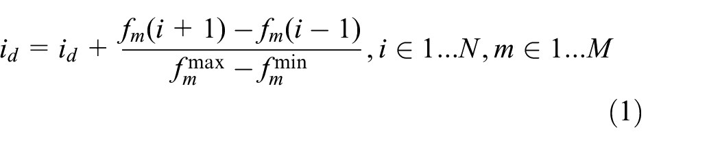
As shown in equation (1), the crowding distance of individual i depends on the difference of $f_{m} (i + 1)$ and $f_{m} (i - 1)$ , without considering the position of the current target individual $f_{m} (i)$ in $[f_{m} (i - 1), f_{m} (i + 1)]$ interval. This is easy to cause the problem that the distance of previous individual $i - 1$ and next individual $i + 1$ is far, but individual i is very close to one of them. For example, $f_{m} (i + 1) - f_{m} (i - 1)$ is equal to $f_{m} (i + 2) - f_{m} (i)$ , but individual i and $i + 1$ are very close. As shown in Figure 2,² individual 2 is close to individual 3.

Figure 2.

The problem of crowding distance.

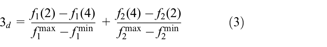
As shown in Figure 2 and equation (1), the crowding distance of individual 2 is:

2_{d} = \frac{f_{1} (1) - f_{1} (3)}{f_{1}^{max} - f_{1}^{min}} + \frac{f_{2} (3) - f_{2} (1)}{f_{2}^{max} - f_{2}^{min}}

(2)

Where, $f_{1}^{max} = f_{1} (1)$ , $f_{1}^{min} = f_{1} (4)$ , $f_{2}^{max} = f_{2} (4)$ , $f_{2}^{min} = f_{2} (1)$ .

The crowding distance of individual 3 is:

3_{d} = \frac{f_{1} (2) - f_{1} (4)}{f_{1}^{max} - f_{1}^{min}} + \frac{f_{2} (4) - f_{2} (2)}{f_{2}^{max} - f_{2}^{min}}

(3)

If $f_{1} (1) - f_{1} (3)$ is equal to $f_{1} (2) - f_{1} (4)$ , and $f_{2} (3) - f_{2} (1)$ is equal to $f_{2} (4) - f_{2} (2)$ , then $2_{d}$ is equal to $3_{d}$ , but individual 2 is very close to individual 3.

As shown in Figure 2, the current crowding distance operator ensures that the previous and next individuals are dispersed as much as possible, but cannot guarantee the dispersion of two adjacent individuals. If all members of the next generation are calculated in the current crowding distance approach, the solutions would not be evenly dispersed. Three NSGA-II improving strategies are proposed in view of this problem. The three improved algorithms are optimized from the perspective of individual geometric position. The difference is that they each refer to the position of the previous individual, the position of the right angle point, and the position of the geometric center.

Side length optimization strategy

If the pervious and next individuals are scattered and the target individuals are far away from the previous individual, the dispersion of the solution set can be greatly improved. As shown in Figure 2, if individual 2 is far away from individual 1 and 4, and individual 3 is far away from individual 2 and 4, the solution set has a great dispersion.

The distance between the current individual and the previous individual is calculated in equation (1), and the formula of side length optimization strategy based NSGA-II (SLOSB-NSGA-II) is shown in equation (4):

i_{d} = \sum_{m = 1}^{M} [\frac{f_{m} (i + 1) - f_{m} (i - 1)}{f_{m}^{max} - f_{m}^{min}} + \frac{f_{m} (i) - f_{m} (i - 1)}{f_{m}^{max} - f_{m}^{min}}]

(4)

Where, $i_{d}$ is the crowding distance, i is the serial number of the current individual, and M is the total number of objective functions.

As shows in Figure 2, the crowding distance of individual 2 calculated by SLOSB-NSGA-II is:

\begin{matrix} 2_{d} = (\frac{CE}{f_{1}^{max} - f_{1}^{min}} + \frac{AE}{f_{2}^{max} - f_{2}^{min}}) + (\frac{BP}{f_{1}^{max} - f_{1}^{min}} + \frac{RB}{f_{2}^{max} - f_{2}^{min}}) \\ = \frac{CE + BP}{f_{1}^{max} - f_{1}^{min}} + \frac{AE + AP}{f_{2}^{max} - f_{2}^{min}} \end{matrix}

(5)

The current individual and the previous individual are made scatter by SLOSB-NSGA-II while the previous and next individuals are also made scatter. This ensures the uniform dispersion of the whole result set.

Diagonal optimization strategy

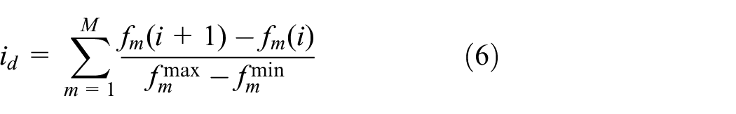
If the target individual is close to the vertex closest to the origin of the largest hyperrectangle formed by the previous and next individuals, the dispersion of the solution set is large. As shown in Figure 2, if individual 2 is close to point E, individual 2 is dispersed from individual 1 and individual 3. The diagonal optimization strategy based NSGA-II (DOSB-NSGA-II) is proposed according to this principle, and its formula is shown in equation (6).

i_{d} = \sum_{m = 1}^{M} \frac{f_{m} (i + 1) - f_{m} (i)}{f_{m}^{max} - f_{m}^{min}}

(6)

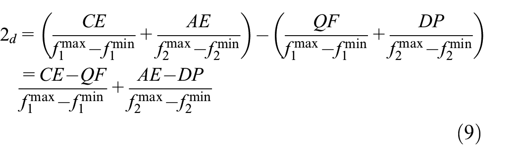
As shown in Figure 2, the crowding distance of individual 2 calculated by DOSB-NSGA-II is:

\begin{matrix} 2_{d} = (\frac{CE}{f_{1}^{max} - f_{1}^{min}} + \frac{AE}{f_{2}^{max} - f_{2}^{min}}) - (\frac{QE}{f_{1}^{max} - f_{1}^{min}} + \frac{PE}{f_{2}^{max} - f_{2}^{min}}) \\ = \frac{CE - QE}{f_{1}^{max} - f_{1}^{min}} + \frac{AE - PE}{f_{2}^{max} - f_{2}^{min}} = \frac{CQ}{f_{1}^{max} - f_{1}^{min}} + \frac{AP}{f_{2}^{max} - f_{2}^{min}} \end{matrix}

(7)

The current individual is made close to the vertex closest to the origin by DOSB-NSGA-II when the distance between previous and next individuals is large, therefore the solution set is dispersed uniformly.

Center optimization strategy

If the current individual is close to the center of the maximum hyperrectangle formed by the previous and next individuals, the solution set has a good dispersion. In Figure 2, if individual 2 is close to the center point O, individual 2 is dispersed from individual 1 and 3. The central optimization strategy based NSGA-II (COSB-NSGA-II) is proposed according to this, and is shown in equation (8).

i_{d} = \sum_{m = 1}^{M} [\frac{f_{m} (i + 1) - f_{m} (i - 1)}{f_{m}^{max} - f_{m}^{min}} - \frac{| 2 f_{m} (i) - f_{m} (i + 1) - f_{m} (i - 1) |}{2 (f_{m}^{max} - f_{m}^{min})}]

(8)

As shown in Figure 2, the improved crowding distance of individual 2 calculated by COSB-NSGA-II is:

\begin{matrix} 2_{d} = (\frac{CE}{f_{1}^{max} - f_{1}^{min}} + \frac{AE}{f_{2}^{max} - f_{2}^{min}}) - (\frac{QF}{f_{1}^{max} - f_{1}^{min}} + \frac{DP}{f_{2}^{max} - f_{2}^{min}}) \\ \frac{= CE - QF}{f_{1}^{max} - f_{1}^{min}} + \frac{AE - DP}{f_{2}^{max} - f_{2}^{min}} \end{matrix}

(9)

The current individual is made close to the geometric center of the hyperrectangle by COSB-NSGA-II when the distance between the previous and the next individuals is large, then the whole solution set is dispersed uniformly.

Algorithm performance comparison

Two-dimensional functions ZDT1-ZDT3 and high-dimensional functions DTLZ1-DTLZ3 are used as objective functions. NSGA-II² and three improved algorithms are used to optimize objective functions. After the optimization, the optimized data are calculated by IGD (reverse generation distance) evaluation function. The IGD evaluation function calculates the convergence and diversity of the algorithm. The smaller the IGD value is, the better the comprehensive performance of the algorithm is. The mathematical formula of IGD is shown as equation (10).

IGD (P, P^{*}) = \frac{\sum dis (x, x^{*})}{| P^{*} |}

(10)

Where, P is the algorithm optimization solution, $P^{*}$ is the mathematical theory solution, and $dis (x, x^{*})$ is the Euclidean distance from point x in P to point $x^{*}$ in $P^{*}$ .

For two-dimensional functions ZDT1, ZDT2, and ZDT3, IGD function results with iteration times of 500, 1000, 1500, and 2000 are counted respectively in order to analyze the influence of iteration times on the results. The maximum, average, and minimum values are shown in Table 1 by repeating the calculation of the above results for 100 times.

Table 1.

Comparison of IGD maximum, average, minimum results of ZDT functions.

Function	Iterations	NSGA-II	SLOSB-NSGA-II	Error/%	DOSB-NSGA-II	Error/%	COSB-NSGA-II	Error/%
ZDT1		0.2699	0.3434		0.2306		0.2624
	500	0.0727	0.0666	−8.3906	0.0441*	−39.3398	0.0663	−8.8033
		0.0106	0.0120		0.0104		0.0146
		0.0677	0.0818		0.0641		0.0648
	1000	0.0217	0.0218	0.4608	0.0240	10.5991	0.0186*	−14.2857
		0.0089	0.0089		0.0107		0.0090
		0.0291	0.0452		0.0231		0.0289
	1500	0.0130	0.0145	11.5385	0.0143	10.0171	0.0126*	−3.0769
		0.0095	0.0084		0.0105		0.0094
		0.0216	0.0158		0.0156		0.0224
	2000	0.0129	0.0101*	−21.7054	0.0115	−10.8527	0.0116	−10.0775
		0.0087	0.0085		0.0090		0.0088
ZDT2		0.7412	0.6547		0.6873		0.7289
	500	0.3223	0.2358	−26.8383	0.2088*	−35.2156	0.3091	−4.0956
		0.0282	0.0238		0.0184		0.0209
		0.6222	0.6214		0.6146		0.6180
	1000	0.1859	0.1413	−23.9914	0.0757	−59.2792	0.0430*	−76.8693
		0.0107	0.0095		0.0117		0.0094
		0.6294	0.6209		0.6500		0.6124
	1500	0.1942	0.0351*	−81.9258	0.1041	−46.3955	0.0596	−69.3100
		0.0097	0.0094		0.0116		0.0090
		0.1298	0.6229		0.6762		0.6091
	2000	0.1133	0.1723	52.0741	0.1013	−10.5914	0.0322*	−71.5799
		0.0088	0.0090		0.0113		0.0088
ZDT3		0.3059	0.3122		0.3066		0.2990
	500	0.1129	0.1051	−6.9088	0.0926*	−17.9805	0.1029	−8.8574
		0.0284	0.0349		0.0406		0.0332
		0.0687	0.0855		0.0870		0.0996
	1000	0.0297	0.0326	9.6743	0.0431	45.1178	0.0280*	−5.7239
		0.0134	0.0156		0.0255		0.0147
		0.0262	0.1116		0.0502		0.0245
	1500	0.0169	0.0244	44.3787	0.0299	76.9231	0.0167*	−1.1834
		0.0131	0.0115		0.0205		0.0127
		0.0422	0.0190		0.0339		0.0197
	2000	0.0148	0.0136*	−8.1081	0.0257	73.6486	0.0145	−2.0270
		0.0113	0.0103		0.0156		0.0119

Where, the bold data are the average results, and the data with * are the best value.

For DTLZ function, the optimization results of 3, 5, 8, and 10 dimensions are calculated respectively. The number of iterations of DTLZ1, DTLZ2, and DTLZ3 are 700, 250, and 1000 respectively according to the characteristics of the function. The calculation is repeated for 100 times, and the maximum, average, and minimum values are shown in Table 2.

Table 2.

Comparison of IGD maximum, average, minimum results of DTLZ functions.

Function	Iterations	Dimension	NSGA-II	SLOSB-NSGA-II	Error/%	DOSB-NSGA-II	Error/%	COSB-NSGA-II	Error/%
DTLZ1	700		0.0290	0.0287		0.0301		0.0279
		3	0.0259	0.0265	2.3166	0.0275	6.1776	0.0257*	−0.7722
			0.0240	0.0242		0.0253		0.0246
			0.0784	0.0706		0.0724		0.0782
		5	0.0762	0.0668*	−12.3360	0.0679	−10.8924	0.0749	−1.7060
			0.0248	0.0627		0.0326		0.0734
			0.0785	0.0708		0.0730		0.0778
		8	0.0764	0.0678*	−11.2565	0.0689	−9.8168	0.0758	−0.7853
			0.0749	0.0642		0.0651		0.0739
			0.0789	0.0727		0.0737		0.0790
		10	0.0770	0.0670*	−12.9870	0.0695	−9.7403	0.0767	−0.3896
			0.0761	0.0626		0.0657		0.0722
DTLZ2	250		0.0785	0.0714		0.0728		0.0759
		3	0.0765	0.0687*	−10.1961	0.0696	−9.0196	0.0704	−7.9739
			0.0741	0.0668		0.0658		0.0656
			0.0776	0.0708		0.0716		0.0787
		5	0.0763	0.0686	−10.0917	0.0680*	−10.8781	0.0751	−1.5727
			0.0747	0.0662		0.0637		0.0726
			0.0785	0.0733		0.0710		0.0779
		8	0.0767	0.0680	−11.3429	0.0672*	−12.3859	0.0764	−0.3911
			0.0748	0.0648		0.0632		0.0744
			0.0794	0.0753		0.0720		0.0786
		10	0.0768	0.0692	−9.8958	0.0692*	−9.8960	0.0763	−0.6510
			0.0750	0.0643		0.0669		0.0744
DTLZ3	1000	3	0.0771	0.0708		0.0769		0.0726
		5	0.0758	0.0682*	−10.0264	0.0693	−8.5752	0.0691	−8.8391
		8	0.0742	0.0650		0.0656		0.0648
			0.0786	0.0719		0.0694		0.0802
			0.0762	0.0687	−9.8425	0.0676*	−11.2861	0.0743	−2.4934
			0.0743	0.0643		0.0660		0.0709
			0.0789	0.0708		0.0771		0.0793
			0.0770	0.0679*	−11.8182	0.0698	−9.3506	0.0764	−0.7792
			0.0756	0.0641		0.0652		0.0753
			0.0787	0.0736		0.0772		0.0786
		10	0.0764	0.0678*	−11.2565	0.0698	−8.6387	0.0759	−0.6545
			0.0742	0.0646		0.0632		0.0748

Where, the bold data are the average results, and the data with * are the best value.

In Tables 1 and 2, overall, the average IGD values of three improved algorithms are smaller than that of NSGA-II, which indicates that the performance of the improved algorithm is superior to the original. It can also be seen from Tables 1 and 2 that the average IGD values of COSB-NSGAII algorithm are smaller than those of original NSGA-II algorithm. When the dimension of the objective function is lower than 5, as for ZDT functions, COSB-NSGA-II has the largest number of best values, as for three-dimension DTLZ, COSB-NSGA-II is also the unique algorithm to have smaller IGD value than NSGA-II, which means the IGD values of COSB-NSGA-II are also better than SLOSB-NSGA-II and DOSB-NSGA-II, indicating that the COSB-NSGA-II has better comprehensive performance.

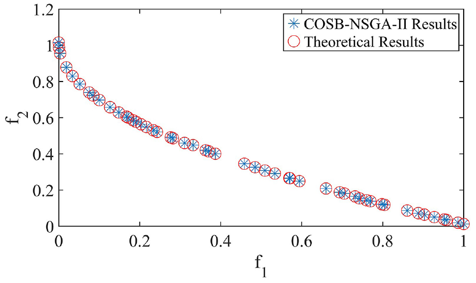
The Pareto frontier results of ZDT1-ZDT3 and DTLZ1-DTLZ3 optimized by COSB-NSGA-II are shown in Figures 3 to 5, and Figures 6 to 8.

Figure 3.

Pareto frontier results of ZDT1 optimized by COSB-NSGA-II.

Figure 4.

Pareto frontier results of ZDT2 optimized by COSB-NSGA-II.

Figure 5.

Pareto frontier results of ZDT3 optimized by COSB-NSGA-II.

Figure 6.

Pareto frontier results of DTLZ1 optimized by COSB-NSGA-II.

Figure 7.

Pareto frontier results of DTLZ2 optimized by COSB-NSGA-II.

Figure 8.

Pareto frontier results of DTLZ3 optimized by COSB-NSGA-II.

Structure optimization of body in white

Body-in-white (BIW) structure optimization is established based on the finite element (FE) model. The frequency design sensitivity analysis (DSA) is firstly carried out, and the design variables are selected according to the DSA ranking results. After that, the BIW neural network surrogate model is established based on the relationship of the design variables with the BIW first torsional mode and static bending-torsion stiffness. Choosing three design variables as objectives: the BIW total mass increment, the first torsional mode frequency increment, and the torsion stiffness increment. Then, optimization functions are established and optimized by COSB-NSGA-II because it performs best on three-dimension optimization problems among three improved strategies, and the most appropriate BIW structure is calculated and verified by mode tests.

Finite element model of BIW

The finite element model of BIW is shows as Figure 9.

Figure 9.

BIW finite model.

The BIW FE model is composed of sheet metal models. The FE model is preprocessed before the simulation. Some unimportant points, lines, surfaces, and holes are firstly deleted in Hypermesh. After that, Quad and Tria are used on two-dimensional mesh drawing of the model. The elastic modulus, Poisson’s ratio, and density of each sheet metal model are assigned according to actual materials. RBE2 and RBE3 units are adopted to take place of spotwelds and bolt connections. The design parameters of the FE model are shown in Table 3.

Table 3.

Finite element model parameters of BIW.

Parameter	Value	Unit
Longitudinal length	2376	mm
Transverse length	3168	mm
Vertical length	2848	mm
Total mass	375.01	kg
front and rear mount distance	1.810	mm
left and right mount distance	1.504	mm
Grid maximum size	10	mm
Grid minimum size	4	mm
Grid minimum Jakobite ratio	1.0
Quadrilateral grid maximum angle	135	°
Quadrilateral grid minimum angle	45	°
Triangular grid maximum angle	120	°
Triangular grid minimum angle	20	°
Grid total number	459,677
Triangular grids total number	41,377
Quadrilateral grids total number	418,300

BIW surrogate model

The improved strategy of NSGA-II cannot be used in the optimization of BIW structure directly, therefore a BIW neural network surrogate model is established based on FE model to describe the relationship of design variables with first torsional mode and bending-torsion stiffness.

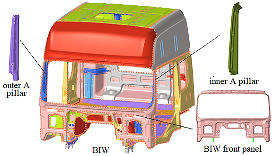
The selection of design variables of surrogate model

Design sensitivity analysis (DSA) is used on the BIW FE model to select design variables of the surrogate model. The design sensitivity is the partial derivative of the DSA result with respect to DSA design variables. The model thicknesses are taken as the DSA design variables and the BIW mode frequency is taken as the DSA result. The design sensitivity of each sheet metal model is calculated by OptiStruct Solver. The DSA results are ranked in order, and the top five sheet models are shown in Table 4.

Table 4.

Sorting results of DSA.

Model	Design sensitivity	Mass/kg	Thickness/mm
BIW front panel	3.027	8.57	1
Inner A pillar	1.471	2.24	1
Outer A pillar	0.515	2.06	1
Longitudinal beam	0.337	10.13	2
Ceiling	0.315	21.41	2

The design sensitivity greater than 0.5 indicates that the model has a great influence on the BIW mode frequency.¹⁸ Therefore, the design variables of the surrogate model are: the thickness of the BIW front panel, inner A pillar, and outer A pillar respectively.

BIW first torsional mode

The first torsional mode and bending-torsion stiffness of BIW are calculated by FE simulation. The first torsional mode is calculated in free conditions. The analysis boundary conditions are unconstrained. The calculation frequency range is set from 0.1 to 100 Hz to avoid rigid body modes which are close to 0 Hz. The first torsional mode of original BIW calculated by OptiStruct Solver is 17.04 Hz, as shown in Figure 10.

Figure 10.

First torsional mode of BIW.

BIW static bending-torsion stiffness

The static bending-torsion stiffness of BIW is calculated as shown in equation (11).

G = \frac{TL}{\arctan (\frac{d_{1} + d_{2}}{B})}

(11)

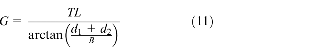
Where, G is the bending-torsional stiffness, T is the loading force, L is the distance between front and rear suspension mounts, d₁ and d₂ are the displacement of loading points respectively, and B is the distance between front left and front right suspension mounts. Physically speaking, T stands for BIW longitudinal length, and B stands for the transverse length. For a BIW, T and B are fixed. If the deformation is smaller under loading, the stiffness of BIW will be larger.

Finite element statics analysis method is used to calculate d₁ and d₂. Two rear suspension mounts are constrained in six degrees of freedom. Two coplane and opposite vertical forces F are applied on two front suspension mounts respectively. Both forces are 1000 N. Boundary conditions are shown in Figure 11.

Figure 11.

Boundary conditions for BIW static analysis.

The result of statics analysis is shown in Figure 12.

Figure 12.

Results of BIW statics analysis.

Neural network surrogate model

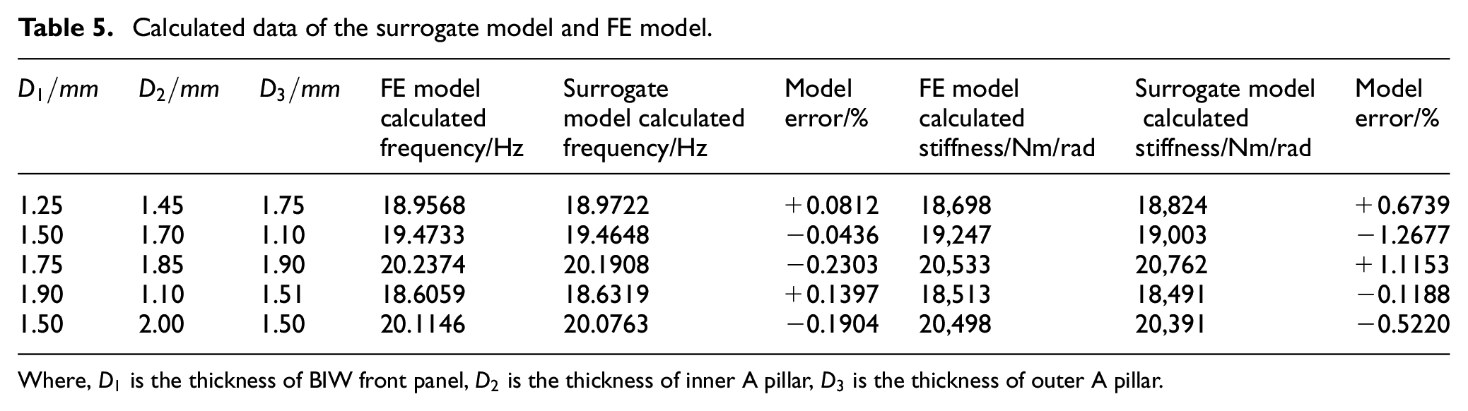
BP artificial neural network surrogate model is established to describe the relationship of design variables with the first torsional mode and static bending-torsion stiffness. Design variables are taken as the input layer of the surrogate model. The first torsional mode and static bending-torsion stiffness are taken as the output layer. The number of middle layer is 7. The BP neural network surrogate model is built with three layers of 3 × 7 × 2 structure. Input layer parameters are selected by interpolation. The design variable with greater influence on DSA results has more interpolation. The thickness of BIW front panel is 1, 1.25, 1.5, 1.75, 2 mm; the thickness of inner A pillar is 1, 1.333, 1.666, 2 mm; the thickness of outer A pillar is 1, 1.5, 2 mm. The parameters of input layer are combined to 60 sets of data. The surrogate model calculated values and the FE simulated values are shown in Table 5.

Table 5.

Calculated data of the surrogate model and FE model.

$D_{1} / mm$	$D_{2} / mm$	$D_{3} / mm$	FE model calculated frequency/Hz	Surrogate model calculated frequency/Hz	Model error/%	FE model calculated stiffness/Nm/rad	Surrogate model calculated stiffness/Nm/rad	Model error/%
1.25	1.45	1.75	18.9568	18.9722	c0.0812	18,698	18,824	+0.6739
1.50	1.70	1.10	19.4733	19.4648	−0.0436	19,247	19,003	−1.2677
1.75	1.85	1.90	20.2374	20.1908	−0.2303	20,533	20,762	+1.1153
1.90	1.10	1.51	18.6059	18.6319	+0.1397	18,513	18,491	−0.1188
1.50	2.00	1.50	20.1146	20.0763	−0.1904	20,498	20,391	−0.5220

Where, $D_{1}$ is the thickness of BIW front panel, $D_{2}$ is the thickness of inner A pillar, $D_{3}$ is the thickness of outer A pillar.

In Table 5, the model error is small, so the neural network surrogate model can be considered correct.

BIW structural optimization

The optimization functions are shown in equation (12).

{\begin{matrix} min f_{1} = \sum_{i = 1}^{3} \frac{D_{i} - d_{i}}{d_{i}} m_{i} \\ min f_{2} = \frac{1}{Mode (D_{1}, D_{2}, D_{3})} \\ min f_{3} = \frac{1}{Stiffness (D_{1}, D_{2}, D_{3})} \end{matrix}

(12)

Where, $D_{i}$ is the thickness of sheet metal model i, the unit of $D_{i}$ is mm. $d_{i}$ is the original thickness of sheet metal model i, $m_{i}$ is the original mass of sheet metal model i, Mode is the first torsional mode of BIW, Stiffness is the static bending-torsion stiffness of BIW. Mode and Stiffness are calculated by surrogate model. $f_{1}$ is the total mass increment of BIW.

The COSB-NSGA-II algorithm is adopted to optimize the BIW optimization functions. The optimal solution is selected based on: the BIW total mass increment is less than 3%, the first torsional mode frequency increment is more than 15%, and the torsion stiffness increment is more than 10%.

The optimal solution set obtained is shown in Table 6.

Table 6.

The optimal solution set.

$D_{1}$ /mm	$D_{2}$ /mm	$D_{3}$ /mm	Mass increment /kg	First torsional mode/Hz	Torsional stiffness/Nm/rad
1.10	1.73	1.65	7.9181	19.6597	19,371
1.33	1.87	1.35	8.9197	19.6591	19,306
1.19	1.78	1.48	8.1512	19.6013	19,107
1.84	1.62	1.84	8.9254	19.8775	19,731
2.00	2.00	1.00	10.8100	20.1813	19,992

For the convenience of model manufacturing and engineering testing, the thickness of the sheet metal models are chose as integer according to Table 6. The thickness of BIW front panel, the inner A pillar, and the outer A pillar is selected as 2.00, 2.00, and 1.00 mm respectively. The trial-produced samples are made and verified by the BIW free mode test.

In the test, the BIW is suspended by hammock and soft rubber rope, and acceleration sensors are installed at the eight corners of BIW to measure the mode data. The first torsional mode is applied by two vibration exciters. The exciting force angle of each vibration exciter is 45°. One vibration exciter is located in the front of BIW, and another is in the rear, as shown in Figure 13. The excitation signal is random initiation signal, and the bandwidth is 500 Hz.

Figure 13.

BIW free mode test.

BIW free mode test values are calculated in LMS TEST.LAB software as shown in Figure 13. The first torsional mode test result is 20.1826 Hz. The surrogate model calculated mode is 20.1803 Hz as shown in Table 6, the model error is 0.01%. Which proves the correctness of the results and the correctness of NSGA-II in BIW structure optimization. First torsional mode test results is shown in Figure 14.

Figure 14.

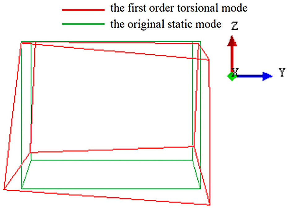
First torsional mode test results.

Conclusions

Three NSGA-II improved algorithms are proposed: side length optimization strategy based NSGA-II (SLOSB-NSGA-II), diagonal optimization strategy based NSGA-II (DOSB-NSGA-II), and center optimization strategy based NSGA-II (COSB-NSGA-II). The performance differences between NSGA-II and the three improved algorithms are compared by ZDT, DTLZ test functions, and IGD values. The results show that the performance of the three improved algorithms is better than original NSGA-II, and COSB-NSGA-II has the best performance among the three improved algorithms.

The surrogate model is established by BIW finite element model and used to describe the relationship between sheet metal model thickness and BIW mass, first torsional mode and static bending-torsion stiffness. The surrogate model and COSB-NSGA-II are used to optimize the BIW structure. The BIW total mass increment is less than 3%, the first torsional mode frequency increment is more than 15%, and the torsion stiffness increment is more than 10%. The optimization results are verified by BIW first torsional mode test. This study provides a reference for the improvement of NSGA-II algorithm and its application in BIW structure optimization.

However, the current research only compares the improved algorithm with the original NSGA-II, and only applies it to the optimization of BIW. The comparison between these improved algorithms and other studies, the diversified evaluation and the application in other engineering aspects need further research.

Footnotes

Handling Editor: Chenhui Liang

Declaration of conflicting interests

The author(s) declared no potential conflicts of interest with respect to the research, authorship, and/or publication of this article.

Funding

The author(s) disclosed receipt of the following financial support for the research, authorship, and/or publication of this article: The authors acknowledge the support from the National Key R&D Program of China (No. 2018YFB0106200).

ORCID iD

Xiao Wu

References

Srinivas

Deb

Multiobjective optimization using nondominated sorting in genetic algorithms. Evol Comput 1994; 2: 221–248.

Deb

Pratap

Agarwal

, et al. A fast and elitist multiobjective genetic algorithm: NSGA-II. IEEE Trans Evol Comput 2002; 6: 182–197.

Zhao

Xue

, et al. Multi-objective classification based on NSGA-II. Int J Comput Sci Math 2018; 9: 539–546.

Verma

Pant

Snasel

A comprehensive review on NSGA-II for multi-objective combinatorial optimization problems. IEEE Access 2021; 9: 57757–57791.

Camara

MVO

Ribeiro

Tosta

MDCR

. A pareto optimal study for the multi-objective oil platform location problem with NSGA-II. J Pet Sci Eng 2018; 169: 258–268.

Azadeh

Pashapour

Abdolhossein Zadeh

Designing a cellular manufacturing system considering decision style, skill and job security by NSGA-II and response surface methodology. Int J Prod Res 2016; 54: 6825–6847.

Attar

Raissi

Khalili-Damghani

A simulation-based optimization approach for free distributed repairable multi-state availability-redundancy allocation problems. Reliab Eng Syst Saf 2017; 157: 177–191.

Sooktip

Wattanapongsakorn

Identifying preferred solutions for multi-objective optimization: application to capacitated vehicle routing problem. Cluster Comput 2015; 18: 1435–1448.

Cortés-Arcos

Bernal-Agustín

Dufo-López

, et al. Multi-objective demand response to real-time prices (RTP) using a task scheduling methodology. Energy 2017; 138: 19–31.

10.

Zhong

Pantelous

Goh

, et al. A reliability-and-cost-based fuzzy approach to optimize preventive maintenance scheduling for offshore wind farms. Mech Syst Signal Process 2019; 124: 643–663.

11.

Zhao

Yan

, et al. Research on cell manufacturing facility layout problem based on improved NSGA-II. Comput Mater Contin 2020; 62: 355–364.

12.

Cao

Batty

Huang

, et al. Spatial multi-objective land use optimization: extensions to the non-dominated sorting genetic algorithm-II. Int J Geogr Inf Sci 2011; 25: 1949–1969.

13.

Martínez-Vargas

Domínguez-Guerrero

Andrade

ÁG

, et al. Application of NSGA-II algorithm to the spectrum assignment problem in spectrum sharing networks. Appl Soft Comput 2016; 39: 188–198.

14.

Zhao

Huan

Zhang

, et al. A novel multi-objective optimization algorithm based on differential evolution and NSGA-II. In: Proceedings of the 2018 IEEE 22nd international conference on computer supported cooperative work in design (CSCWD), Nanjing, People’s Republic of China, 9–11 May 2018, pp.570–575. New York: IEEE.

15.

Yuan

Dai

GM.

The improved NSGA-II based on reverse learning mechanism. In: Proceedings of the 2015 international industrial informatics and computer engineering conference (IIICEC), Xian, People’s Republic of China, 10–11 January 2015, pp.589–593. Atlantis Press.

16.

Fettaka

Thibault

Gupta

A new algorithm using front prediction and NSGA-II for solving two and three-objective optimization problems. Eng Optim 2015; 16: 713–736.

17.

Zhang

Qian

Multi-objective optimization for materials design with improved NSGA-II. Mater Today Commun 2021; 28: 102709.

18.

Yuan

, et al. Sensitivity of multistage fill slope based on finite element model. Adv Civil Eng 2021; 2021: 1–13.

Improved NSGA-II and its application in BIW structure optimization

Abstract

Keywords

Introduction

NSGA-II

Fast nondominated sorting approach

Crowding distance

Elitist-preserving approach

Improved NSGA-II

The shortcoming of NSGA-II

Side length optimization strategy

Diagonal optimization strategy

Center optimization strategy

Algorithm performance comparison

Structure optimization of body in white

Finite element model of BIW

BIW surrogate model

The selection of design variables of surrogate model

BIW first torsional mode

BIW static bending-torsion stiffness

Neural network surrogate model

BIW structural optimization

Conclusions

Footnotes

Declaration of conflicting interests

Funding

ORCID iD

References