
Abstract
This paper attempts to print irregular 3D objects on a freeform surface. Notably, it is inevitable to cause errors when creating a specific object shape in simulated and real-life scenarios. This is mainly attributed to the unique characteristics of the materials adopted, which tend to develop different deformations properties. Nevertheless, since the simulated model provides a clue regarding the coordinates of the deformed shape, it is adopted as an essential indicator in estimating accurate real-world coordinates. Concretely, this paper presents a complete system that is capable of reconstructing the detailed surface coordinates in real-time conditions. To verify the effectiveness of the proposed method, a metal board is used as the primary material to create different curvatures physically and virtually. In particular, the real-time performance of the overall 3D surface reconstruction has been experimentally evaluated using several tools, such as KUKA KR90 R3100 robots, HoloLens 2, displacement sensor, and ArUco markers. Consequently, both the quantitative and qualitative results are presented to demonstrate the feasibility of the proposed method. Furthermore, the experimental data obtained manifest that there are significant differences between the simulated and the real-world coordinates. Thus, the findings of this study provide an insightful outlook and lay down several important implications for future practice.
Classifications
Computer programing, system and service; Methodology, apparatus, experimental design
Introduction
Owing to advances in machine learning and artificial intelligence, the development of fully automated with a highly accurate 3D reconstruction of objects has been receiving increasing attention from various research fields. One of the early works that conducted the 3D measurement using a laser scanner and rangefinder is by Shi et al. 1 The target of the experiment is both the large-scale bending plate and small complex scenes where several objects (i.e. mouse, keyboard, bottle, etc.) are placed stationery at a fixed position. Then a robotic arm is mounted on a guide rail such that a specific route is designed for the robotic movement. Then, two stereo cameras are placed on the robotic arm to capture top-down viewpoint images. Concretely, the 3D scanner measures partial sections, whereas the laser rangefinder provides the poses of the scanner in different view alignments. The results reported also serve as the benchmark for future work in performing this kind of experiment.
Recently, Bai et al. 2 extends the work of Shi et al. 1 by expanding the experimental setup in improving the accuracy and computational speed of the measurement. Concisely, two guide rails and an infrared 3D scanner are considered. To evaluate the robustness of the proposed method, a large non-smooth surface steel plate is treated as a complex large scene such that the measuring task is more challenging. However, similar to the previous work, 1 these measuring instruments require a sufficiently large physical operating workspace.
On the other hand, to perform the 3D surface reconstruction of the plant seed, 3 proposed to utilize robotized turntable systems to handle and rotate the seed. A camera is placed in front of the seed such that a total of 36 images will be collected with the step degree of 10°. This method facilitates an affordable 3D imaging technique and the promising experimental results demonstrate the robustness of the method. A similar 3D image reconstruction method was applied to another agricultural product, viz, ham.4,5 Succinctly, the ham object is placed on a rotating display stand horizontally and vertically and rotated at a constant speed. Then, an automatic semantic segmentation technique, namely Mask-RCNN (Regional Convolutional Neural Network) 6 is applied to construct the object’s 3D model. To improve the object segmentation task, reliable camera tracking is adopted on top of the Mask-RCNN technique is demonstrated in Hoang et al. 7 to achieve a semantic 3D map.
A real-time 3D reconstruction display had been performed effectively using HoloLens and Kinect sensors. Since HoloLens provides a built-in rendering virtual imagery display, a consistent rate of 60 fps allows a better user experience in terms of the sense of the presence of virtual objects. On another note, to enable the automated digitization of museum artifacts, 8 proposed a method such that an automated, accurate, and dense 3D reconstruction system can be utilized to focus on small objects (<30 cm). Concretely, the system includes stereo imaging networks and robot inverse kinematics. Then, several mathematical modelings are introduced to enhance the objects’ postures effect.
On another note, several previous works develop 3D reconstruction systems for small-scale smooth or complex objects.9–13 Specifically, in Zhao et al., 9 the coordinate transformation between the robot and the laser scanner had been investigated by suggesting the technique of reverse engineering. Recently, a low-cost and portable reconstruction system is introduced by Hosseininaveh Ahmadabadian et al. 14 Particularly, it contains a pattern projection system, digital camera, raspberry pi, and mobile phone. The system has been evaluated on texture-less objects such as the dude statue, Cyrus tomb statue, and paper cone. Promising results were reported when compared with the measurements obtained from a compact laser scanner. However, a series of systematic procedures are required for equipment calibration.
In short, the importance and originality of this study are summarized as follows. First, this study makes a major contribution in demonstrating an efficient sampling method that enables the acquisition of a small amount of data points in reconstructing an accurate dynamic curved surface executing in real-time. Secondly, inspired by Lyngby et al., 15 a novel efficient and accurate system is introduced to scan the twisting and bending state of a large-scale metal sheet bent by industrial robots. We provide empirical proof of our method by comparing the results produced by HoloLens to robotic laser scans of fabricated models. Last but not the least, promising experiment performance demonstrated that the proposed solution outperformed the simulated model. Note that, the experiments herein performed the results for a specific axis of the robot arm and were limited to a certain range of rotational angles.
This paper is structured as follows: Section 2 describes the experiment preparation and detailed procedure regarding the realization of the real-time curved surface using HoloLens and displacement measurement sensor. Section 3 provides the evaluation metric to examine the effectiveness of the proposed method. Section 4 reports the experimental data with analysis. Both the quantitative and qualitative results are discussed. Finally, a summary is presented in Section 5.
Theory and design
Apparatus preparation
The apparatus involved in the dataset elicitation comprised two robot arms, a piece of sheet metal, a 2D near-range laser scanner, HoloLens 2, and ArUco markers. The following subsections describe each apparatus used in the experiment in detail.
Metal sheet and robot arm
The metal sheet is used as the key material to verify the effect in 3D surface reconstruction because it can be easily bent and shaped. Besides, it is known as one of the building materials that can create rigid and long-lasting structures. The dimension of the metal is 600 cm (Length) × 90 cm (Width) × 0.3 cm (Thickness). The metal material is shown in Figure 1. The experiments are carried out on two six-axis articulated industrial robots KUKA KR90 R3100 Extra. Each robot arm is equipped with high precision and high payload robots (i.e. 90 kg) at a reach of up to 3100 mm. The graphical illustration of the robot arm is shown in Figure 2.
The compound metal as the target object.

Graphical illustration of the two robot arms KUKA KR90 R3100 Extra.
The two robot arms are mounted on an 8-m track, as portrayed in Figure 2. All the robot’s movements have been programed by the robot language of the KUKA software add-on, PLC mxAutomation (MxA), such that it will move to a few specific pre-configured positions to achieve data point collection for the distance information. Real-time communication is enabled between the robot controller and an external system (i.e. a computer). There are two reasons to implement the proposed approach on this robot: (1) it has been widely used in industry due to the system robustness and reliability, and; (2) it can be easily transferred and reproduced on other robots. In this paper, the comparison of current 3D reconstruction using HoloLens with the proposed approach is quantified to validate the performance improvement.
Particularly, in evaluating the system’s robustness, a random bending shape is selected in this study. The metal bending process is performed by using two big-scale robot arms, whereby one side of the metal is held by one of the robot arms to cause it to bend at an angle and form the desired curvature, while the other side is anchored to a mounting plate to secure the metal surface. The robot arm’s translational movement and orientation rotation is triggered to manipulate the metal to create different curved surfaces.
Placement of ArUco markers
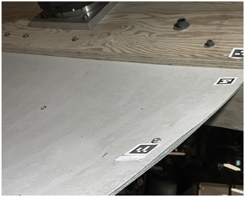
To obtain the metal bending shape numerically, the subsequent step utilized the ArUco marker by placing the marker on the metal surface for sparse position acquisition. In brief, ArUco markers are developed by Garrido-Jurado et al. 16 and his team and were initially designed for camera pose estimation application. The ArUco markers are explicitly designed as visual features for localization, whereby they need to be printed to place on the desired environment space. An ArUco marker is a square fiducial marker encircled by a thick black border and an inner binary matrix that determines its unique marker identifier. The sample for the ArUco marker is shown in Figure 3, which can be generated from this site. 17 The Aruco library is a well-developed OpenCV open-source software that has been widely adopted to estimate the pose of the 6DoF marker from augmented reality fiducials. In total, 45 markers with each unique ID are generated. Amongst, 42 of them are sticked and aligned along the two horizontal edges of the metal, such that each edge contains 21 markers. The separation between the marker pairs is about 25 cm. Some spaces are reserved between the markers and the metal edges, viz, about 3 cm. While three ArUco markers are for positional reference and one ArUco marker is used as the reference point for world coordinate space. The illustration of the placement of the ArUco markers is shown in Figure 4.

Sample of ArUco markers.
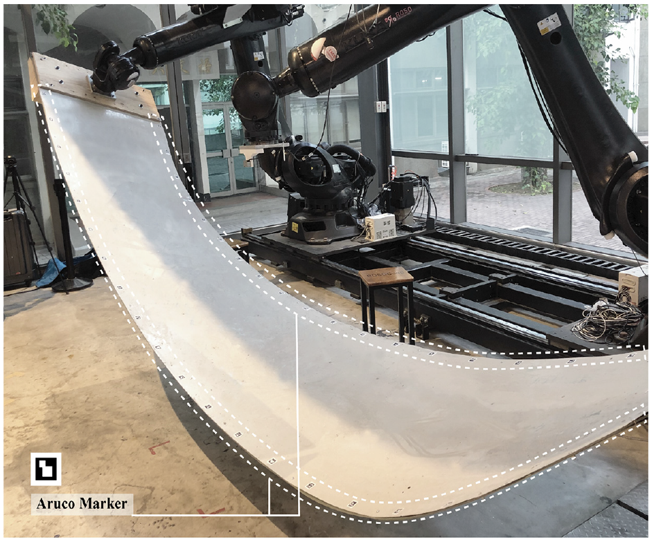
Illustration of the placement of the ArUco markers on the metal board.
Robot calibration
Before measuring the coordinates of the ArUco markers, an offline robot setup is performed to calibrate the robot flange and the measurement tool (i.e. laser range sensor). This step is critically important to precisely derive the relative position between the laser sensor and the robot base coordinate systems. The 2D laser sensor (SICK, OD Mini) projects a wavelength of 635-nm laser lines onto the target object’s surface. The distances measured vary from 50 to 150 mm and the accuracy obtained within the distance range is about 1000 mm. The laser sensor is attached and fixed to the robot’s flange.
During the calibration process, a calibration grid is placed to be fixed in a static position to allow accurate transformation between the laser scanner and the robot coordinate system. Therefore, a simple and robust tool center point calibration strategy is conducted. Specifically, the tool center point calibration is performed manually by moving the robot, letting the tool center point of the robot arm brush against a fixed point in the environment. The fixed point is basically the tip of a nail. The tool center point needs to brush against the tip of the nail with high precision and from four different angles. Conventionally, the position vector of the tool center
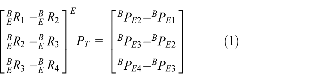
where
As such, the coordinate of the tool center point can be calculated by the robot in relation to the robot’s tool flange coordinate system. The resulting accuracy of robot calibration employing this method is about ±1 mm. Note that, the resultant accuracy is calculated by comparing the resultant solution obtained by solving equation (1) that requires four different robot poses with the known coordinates of the tip of a nail.
Data elicitation
This section describes the data point acquisition step from the metal surface. To obtain accurate coordinates of certain curvature metal surfaces and measure the relative pivoting angle, the software required are Rhino and Grasshopper, which allow the automated simulation process and facilitate the basic structural modeling. The following subsections provide the detailed steps to elicit and derive the real-world coordinates of the metal surface, which include: (1) metal board translation and rotation; (2) marker information retrieval using HoloLens; (3) construction of curves using Rhino and Grasshopper; (4) simulation and refinement of the metal surface; (5) extraction of surface normal’s by offsetting; (6) coordinates acquisition from the subdivided surface using a laser sensor and robot arm, and; (7) derivation of matrix transformation from pixel coordinates to real-world coordinates. A flow diagram is provided in Figure 5 to summarize the methodology proposed for enhancing the real-world coordinates of the metal board.

Flow diagram of the proposed method.
Translation and rotation of metal board
To change the apparent curvature of the flat metal sheet, the robot arm is utilized. In particular, the robot arm that holds one side of the metal sheet is translated by a position vector of (
Marker information retrieval using HoloLens
This step requires Microsoft HoloLens 2 to establish the coordinate system to map to the real-world location. HoloLens is known as one of the quick decision-making tools for creating real-time 3D space. Compared to HoloLens 1, version 2 offers a larger field of view of up to 52° and higher resolution (i.e. 2048 × 1080 pixels). To achieve this, a printed QR code is placed on the edge of the metal board to serve as the reference point. The QR code is utilized in this experiment because it is identified as the most convenient recognition method that is feasible in implementing augmented reality applications. During the holographic visual initialization, HoloLens 2 renders the data detected as holograms using a coordinate system.
As for the coordinates of the two edges of the metal, the HoloLens is adopted to digitize the model by scanning the 42 ArUco markers. Based on the simultaneous localization and mapping (SLAM) algorithm implemented in the HoloLens using the fusion data from the build-in Inertial Sensors (IMU) and depth camera, HoloLens can estimate an object’s location in 3D space from the dead reckoning process. Therefore, a marker-based localization method for the HoloLens is sufficient to perform the localization augmentation for coordinates estimation of the two edges of the metal by scanning the ArUco markers that stick on both edges of the metal. After scanning all the ArUco markers, a virtual representation of the metal sheet can be constructed using the HoloLens plugin for grasshopper, Fologram, which functions in converting the data points scanned into points within the Rhino model space. Finally, the metal shape can be reconstructed in the 3D space with the knowledge of localization information generated from the HoloLens and the 3D poses from the scanned ArUco markers. Note that the distance between the HoloLens and the ArUco markers is held constant within 50 cm to capture the ArUco markers in retrieving the transformation information for 3D reconstruction calculation.
The example of attaining the coordinates information using HoloLens is shown in Figure 6.
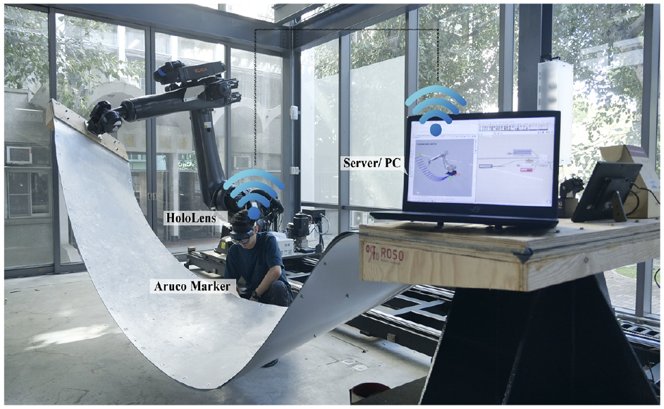
Illustration in attaining the coordinates information using HoloLens.
Construction of curves using Rhino
Since the Grasshopper plugin Fologram enables a two-way data stream that can render geometry in the computer-aided design (CAD) environment on the HoloLens, it allows direct 3D feedback superimposed on reality from a digital CAD model. By doing so, the curve of the metal board can be dynamically simulated by generating surface geometry through the augmented display. The example of the resultant geometry modeling generated from the proposed algorithm in this study is shown in Figure 7. The derivative patterns are created using the parametric modeling software, viz, the Grasshopper plug-in for Rhinoceros.

The algorithmic design tools Grasshopper.
Simulation and refinement of metal board surface
Note that the previous stage only considers the data points collected from the two sides of the metal board. Hence, the current 3D reconstructed metal board may not be exact values in the real-world scenario as there is some variability when estimating the coordinates using the HoloLens’ SLAM algorithm. Besides, since limited data points are considered in the surface reconstruction (i.e. 42 points), it exists some differences in estimated and actual measurements.
Therefore, to acquire the detailed coordinates of the irregular surface, this study proposed a systematic procedure to yield an accurate 3D reconstruction of the metal board. In this step, the plane is subdivided into X × Y by partitioning the grid equally for both the longitude and latitude directions. In general, the subdivision process is done by dividing the straight line connecting the pair of two points from two sides, as shown in Figure 8 by using equation (2).
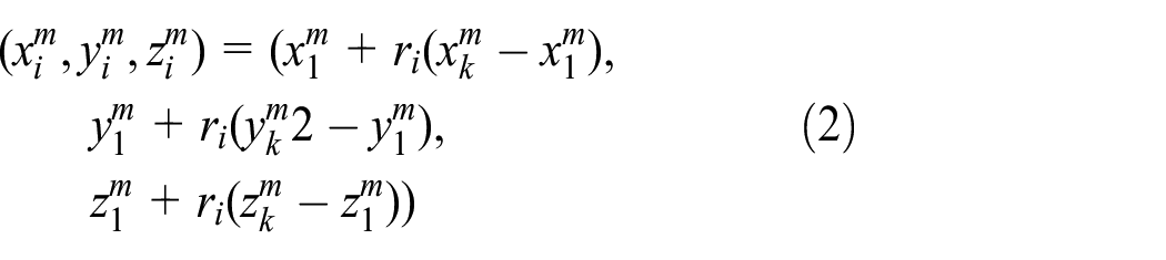
where

Illustration of equally subdividing the grid points for each pair of curves.
The above-mentioned subdivision process can be performed on the Grasshopper surface generation using the built-in subdivision tool. Concretely, the surface is simulated such that it can be reparametrized and redistributed to the UV-grid by using the normal Loft command in the Rhino software. However, although the mesh points of the curved surface can be obtained by the tools provided in the Rhino software, there remains a disparity in the measurement accuracy between the simulated and the real-world points. Thus, the following subsection attempts to improve the simulated points approximation such that it is closer to the real-world points. Succinctly, the correction of mesh points elicited from the previous section can be automatically adjusted and calibrated by exploiting a laser sensor and robot arm with the following sections.
Extraction of surface normal’s by offsetting
In order to obtain the position for the laser scanning process using the robot arm, the offset values are computed as an aid for the coordinates elicitation, aiming to keep a constant distance along an estimated vertex normal of the surface defined by

where
Coordinates acquisition from the subdivided surface using a laser sensor and robot arm
In this stage, the real-world coordinates of the subdivided surface are acquired using a 2D near-range laser range sensor with the assistance of a moving robot arm. As the sensor’s displacement has been calibrated previously, the target position depicted from the robot base reference system can be directly acquired from laser sensor data. As illustrated in Figure 9, the laser sensor is mounted and fixed on the robot arm such that it can be moved over the curve surface by just controlling the robot arm and moving to the offset surface
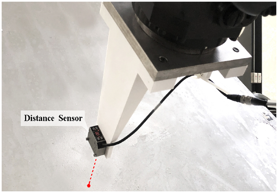
The laser sensor mounted on the robot arm for distance measurement.
3D metal surface reconstruction correction by using laser distance of grid points
In this section, the precise coordinates of the metal surface in the real world are calculated by adjusting the offset surface calculated from Section 2.2.5 using the laser distance obtained in Section 2.2.6. Hence, the parametric form of the metal surface is calculated by the equation below:

where
Experiment setting
To investigate the difference between the simulated coordinates manipulated on Rhino software and the real-world coordinates of the curved surface, a comparison of their mesh points coordinates is calculated. The procedure elaborated in Section 2 is repeated 10 times to produce different curved surfaces. The reason for repeating the experiments is to provide relatively conclusive evidence as it can enhance the data generalization and reliability. Concisely, the curved surface can be created by configuring the amount of translational movement and orientation rotation of one of the robot arms. Specifically, the following analysis investigates the robustness of the proposed method from two scenarios, viz, large and small twisting effects, denoted as
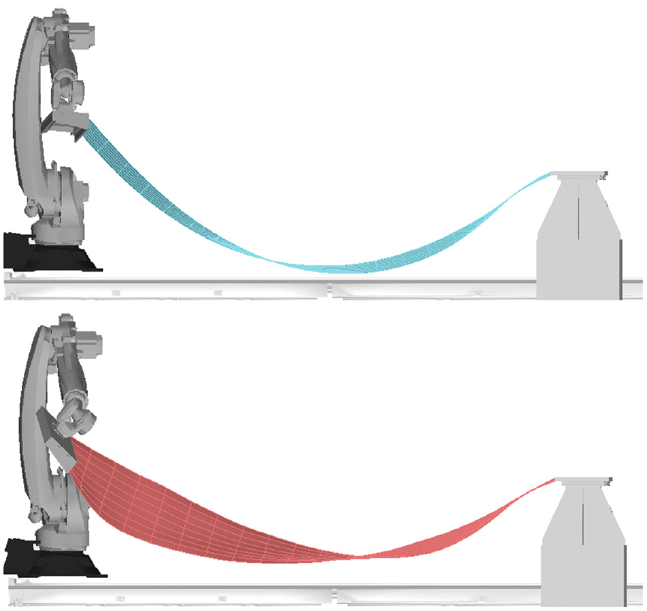
Illustration of (top) small and (bottom) large twisting effects.
Statistical tests
To measure the robustness of the proposed method, the simulated surface output generated by the proposed method is compared to the surface estimated by the HoloLens. In short, all 152 points are compared correspondingly. In total, six quantifying distance metrics are introduced to validate the effectiveness of the proposed method. Concisely, the distance measurement metrics include Hausdorff Distance (HD), 19 Partial Curve Mappingx (PCM), 20 Discrete Frechet Distance (DFD), 21 area, 22 Curve Length (CL), 23 and Dynamic Time Warpingy (DTW). 24 Noticed that, the closer the distance computed, indicating the better the performance of the proposed method.
1. Hausdorff Distance (HD):
The distance measurement between the two discrete surfaces

where
2. Partial Curve Mappingx (PCM):
This measurement utilizes the concept of matching the area of a subset between the two curves and the corresponding computed curve is updated iteratively. The calculation of PCM computes the curve mismatch error as in equation (6):
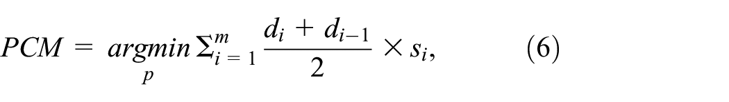
where

Details of the algorithm to calculate PCM can be found in Witowski and Stander. 20
3. Discrete Frechet Distance (DFD):
To calculate the shortest distance in-between two curves 21 and the formulations are defined as defined in equation (8).

4. Area:
To calculate the area between two curves in 2D space as referring to Jekel et al., 22 the area between two curves can be estimated using a trapezoid of the coordinates of the points from two curves as defined in equation (9).

where
5. Curve Length (CL):
This method assumes that the only true independent variable of the curves is the arc-length distance along the curve from the origin.

6. Dynamic Time Warpingy (DTW):
This metric calculates the non-metric distance between two time-series curves based on Levenshtein distance by recursively computing the equation below:

where

where
Descriptive analysis
To summarize the entire mesh points obtained from both the simulated and real-world calibrated coordinates, an analysis is performed subsequently, namely, the descriptive analysis. Concisely, two key metrics are considered, viz, mean and standard deviation. The mean, also known as the average, is calculated by adding all the distances obtained between the two coordinate sets and then dividing by the number of points. On the other hand, the standard deviation is the most commonly used measure of dispersion as it concludes the spread of data points about the mean. The equations of mean and standard deviation are depicted as follows:


To further examine the effectiveness of the proposed method, the rectangular prism-shaped metal board is partitioned into 19 segments along the longitudinal direction. Since there are 152 points on the metal board, each of the eight points is viewed as a composite segment, as illustrated in Figure 11. As such, more local region information can be extracted and analyzed. From this analysis, it is hypothesized that the middle part of the metal board has the largest curvature, leading to the highest erroneous. This is because the deformation of the metal plate seems obvious when the force is applied from one side, while the other side is held constant. To reveal the deformation characteristics and verify the accuracy of each measured mesh point, a detailed analysis is reported in Section 4 later.

The metal that segmented into 19 × 8.
Results and discussion
This section highlights some important findings observed throughout the experiment, including quantitative and qualitative analyses. Concretely, Table 1 presents the mean of the six distance measurements discussed in Section 3.1, which computed the distance difference between each pair of the Rhino simulated and the laser sensor-derived mesh point coordinates. Note that Table 1 portrays the average results for both the scenarios of large and small twisting effect, denoting as
Mean results for the six distance measurement metrics when comparing the points between the Rhino simulated and laser sensor derived points for the metal boards with large twisting (

Concretely, it can be seen from Figure 13 that the trend line for the HD, DFD, DTW, and area are similar. For instance, the distance measures for the third quarter (segments #9–14) of the metal board have relatively lower measurement distances. This is tallying to the values generated by CL in Table 1, whereby the (segments #9–14) produce the smallest distance difference ranging from 0 to 0.01. This implies that the twisting effect is relatively low in the third quarter of the metal board.
On the other hand, the sub-figures for PCM and CL have obvious spikes at the fourth quarter metal board segment (#15–19), indicating a large estimation difference between the simulated and real-world mesh point coordinates. This is because of the characteristics of the compound material of the metal board. Since the metal board comprises four pieces of metal plate, a large twisting effect causes a significant protruding impact on the fourth metal board segment, as shown in Figure 12. Nevertheless, the rest of the segments can approximate the coordinate points accurately.

The uneven surface curve of the metal board.
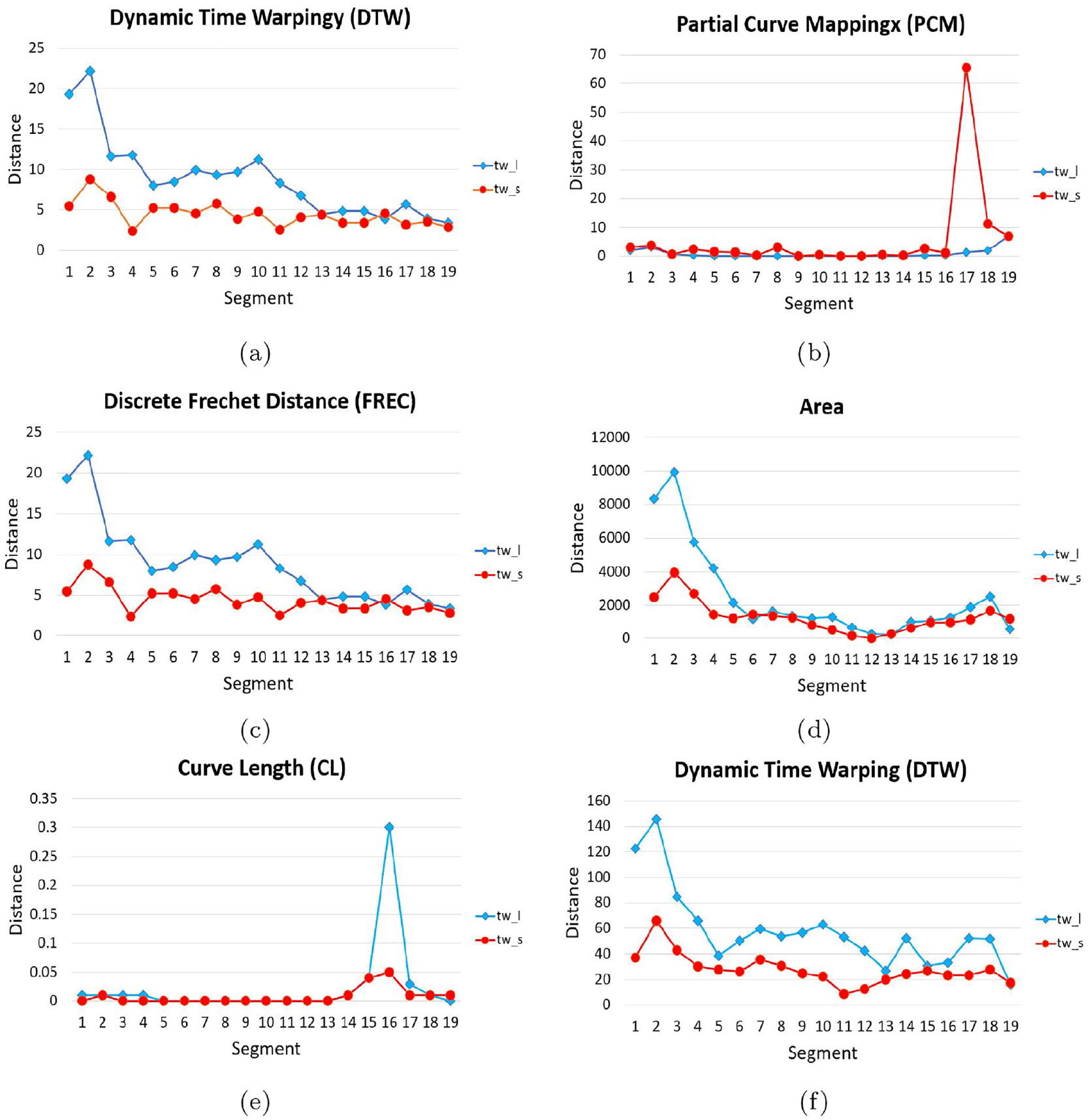
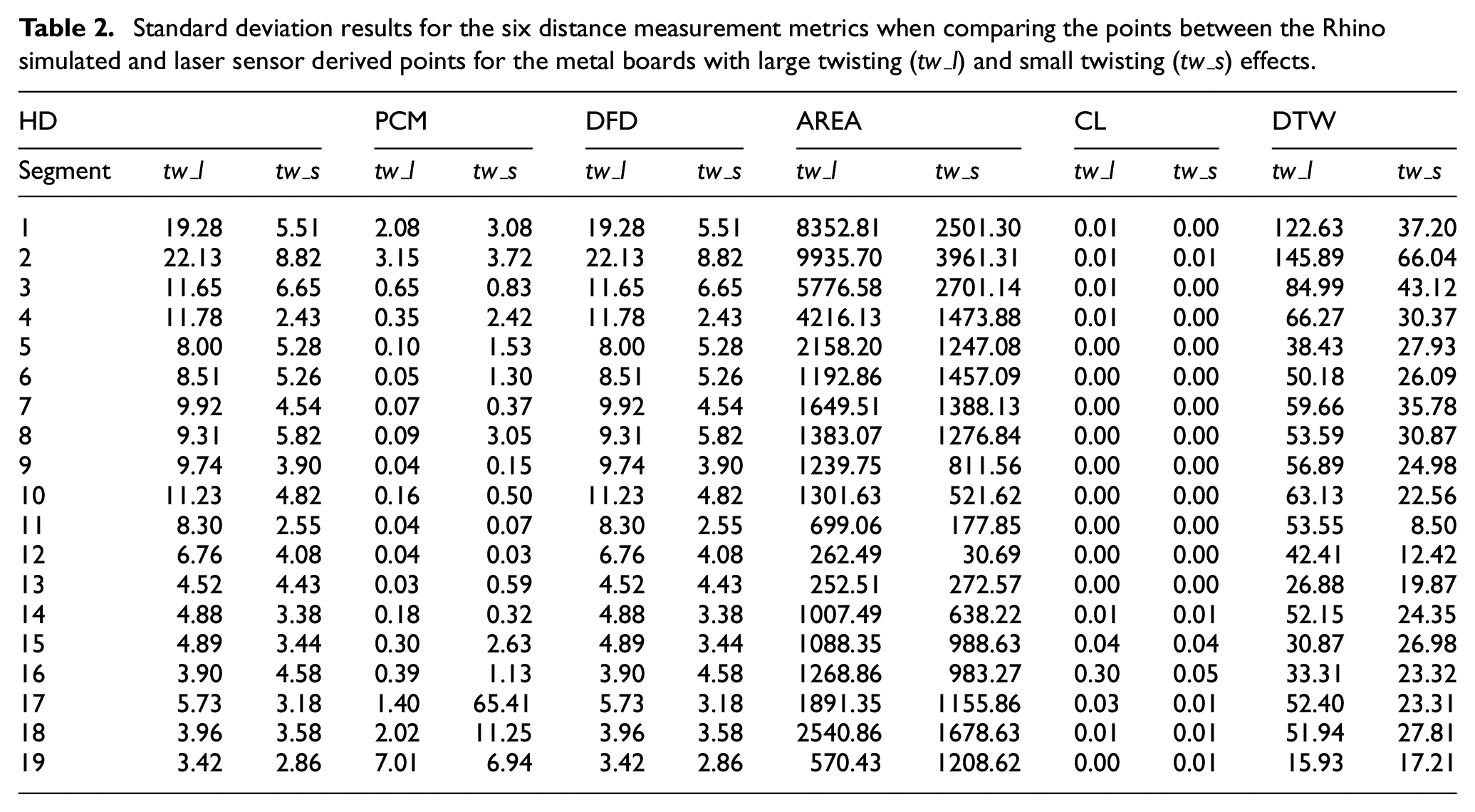
Besides, this study also demonstrates that the proposed method works can be applied to both large and small twisting angles. This can be evidenced by the sub-figures in Figure 13 that the trend of the two lines is similar. In addition, the corresponding standard deviation between all the 152 pairs of points is averaged and reported in Table 2. Figure 14 provides a clear visualization regarding the impact in terms of standard deviation for the different segments when comparing large and small twisting metal boards. It is noticed in Figure 14 that the first half of the metal board has significantly large standard deviation values when applying a larger twisting effect. Interestingly, it can be seen that for the PCM metric, there is an obvious spike at segment #17 for the small twisting metal board due to the protruding effect of the metal materials.
The mean results of different distance measurement metrics of the large and small twisting metal boards when comparing the simulated and derived points: (a) Hausdorff Distance (HD), (b) Partial Curve Mappingx (PCM), (c) Discrete Frechet Distance (FREC), (d) area, (e) Curve Length (CL), and (f) Dynamic Time Warping (DTW).
Standard deviation results for the six distance measurement metrics when comparing the points between the Rhino simulated and laser sensor derived points for the metal boards with large twisting (

The standard deviation results of different distance measurement metrics of the large and small twisting metal boards when comparing the simulated and derived points: (a) Hausdorff Distance (HD), (b) Partial Curve Mappingx (PCM), (c) Discrete Frechet Distance (FREC), (d) area, (e) Curve Length (CL), and (f) Dynamic Time Warping (DTW).
Figure 15 portrays the curved surface of the metal board. The red dots denote the coordinates of the Rhino simulated points whereas the real-world coordinates are annotated as blue crosses. This visual representation further affirms the results tabulated in Table 1, where the pair of points at certain parts metal board has a relatively larger distance than the other parts. Thus, these findings have important implications for developing an automatic scanning system capable of reconstructing accurate, dense, and pixel-wise surface curvature. To verify the accuracy of this system, the paper uses a custom-made extruder attached to the end of the robotic arm that prints 3D objects in varying freeform surfaces, as depicted in Figure 16. Moreover, the final design of 3D objects as depicted in Figure 17.
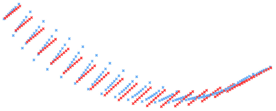
The point coordinates of the metal board when comparing the (red) simulated and (blue) real-world scenarios.

3D printing on freeform molds.

The point coordinates of the metal board when comparing the (red) simulated and (blue) real-world scenarios.
Nevertheless, this observational study raises intriguing questions regarding different types of deformations. In future investigations, one of the potential directions is to reduce the control points in increasing the curvature of the surface. Besides, other types of material with distinct properties can be considered to replace the metal board, like fabric, wood, and plastic. For the apparatus used, the usage of HoloLens 2 can be replaced with other types of devices such as a CCD or CMOS camera that is cost-effective. In addition, to resolve the protruding effect from the experiment results obtained, a comprehensive study regarding the twisting angle of the board can be investigated to further extend the generalization of the proposed method.
Conclusion
Despite estimating the geometry of a huge and freeform object being relatively crucial due to the hardware limitations such as the portability and the detection range of the sensors, this study proposes an end-to-end real-time, and accurate surface reconstruction system. The effectiveness of the proposed method is verified when evaluating different curvatures with unique 3D printing of irregular objects on a freeform surface. The empirical findings in this study demonstrate that the simulated surface visualized on the Rhino software has a significant difference compared to the real-world coordinates. Therefore, the insights gained from this study may be of assistance to suggest an effective solution for simulating the desired shape. Succinctly, the numerical performance and the supplement graphical representations reported in the paper summarized from the 152 pairs of points demonstrate the viability of the proposed method. Concretely, six distance measurements (i.e. Hausdorff Distance, Partial Curve Mappingx, Discrete Frechet Distance, area, Curve Length (CL), and Dynamic Time Warpingy) conveyed the reasonably promising result that primarily retrieved the curvature information via the HoloLens and ArUco marker. Thereupon, future directions point toward a detailed investigation into the combination of machine learning techniques with simulation modeling that aims in refining the precise coordinates of a freeform surface. Through the training process of the machine learning model, the simulated curvature can be enhanced by making it closer to the real object. However, it requires a large number of data sets that are sufficient to build a robust machine learning model.
Footnotes
Handling Editor: Chenhui Liang
Declaration of conflicting interests
The author(s) declared no potential conflicts of interest with respect to the research, authorship, and/or publication of this article.
Funding
The author(s) disclosed receipt of the following financial support for the research, authorship, and/or publication of this article: This work was funded by Ministry of Science and Technology (MOST) (Grant Number: MOST 110-2222-E-035-003-MY2, 110-2222-E-035 -003 -MY2, 111-2221-E-035-059-MY3, and 111-2221-E-A49-034-MY2).