
Abstract
Automatic driving technology has developed over time and the path-following problem for four-wheel independent drive electric autonomous vehicles (4WID-EV) is a topic of increasing interest. During the path-following process, a consideration of uncertainties in vehicle modeling including parameter variation, modeling error, and external disturbances is made, which have an important effect on path-tracking performance. As so, we proposed a new path following control strategy that can be applied to robotics applications. First, it was determined to establish a 2 DOF dynamic model and path following error model, and were then converted to yaw angle tracking problems. Therefore, the desired control input of steering angle was obtained via yaw angle tracking controller. To estimate and compensate the uncertainties associated with systems, the nonlinear extended state observer (NESO) was designed while the NTSM controller was used to realize yaw angle tracking. Next, considering the system stability, a sliding mode controller with modified reaching law was used to obtain the desired additional yaw moment. Then, the optimized torque distributor was designed for allocating optimal tire forces. Finally, the simulation experiments were carried out in Matlab/Simulink and Carsim joint simulation platform. In conclusion, the proposed control scheme exhibits highly accurate path following as well as strong robustness to speed, tire-road friction coefficient and external disturbance.
Keywords
Introduction
Recent decades have seen a significant advancement in the automobile industry which significantly improved the lives of ordinary people. 1 Thanks to this, transportation has become more convenient, which has also played a great role in promoting the development of the overall national economy. However, it should be noted that the development of the automobile industry has brought many “side effects,” such as environmental problems, energy problems, traffic congestion, traffic safety, and so on. Therefore, many countries are vigorously developing new energy vehicles. In numerous new energy vehicles, it is generally acknowledged that electric vehicles (EVs) will become the dominant form of transportation in the near future, 2 which have the following advantages compared with conventional internal combustion cars: no CO2 emission, faster acceleration, and easier to control. According to different powertrain system layouts, electric vehicles can be divided into centralized drive EV and distributed drive EVs. The former is based on the development of traditional internal combustion cars. The main difference between centralized drive EV and internal combustion cars lie in the use of a motor instead of an internal combustion engines as power sources. And EVs with distributed drives are distinguished into two main categories: EVs with in-wheel motors and EVs with motors nearby the wheels. The EV driven by an in-wheel motor is especially suitable for the development and application of automatic driving technology because of its simple structure and easy to control.
Among many distributed drive autonomous EVs, one with four independent drive in-wheel motors and an active steering system1,3 (4WID-EV) has attracted the attention of researchers due to its advantages in maneuverability and flexibility. Path following is one of the most important areas of research when it comes to autonomous vehicles. 4 Tracking reference path with the minimum lateral and orientation error is the main characteristic concerning path following. During the whole tracking process, we need to consider not only the longitudinal control but also the lateral control. For simplicity, we assume that the longitudinal speed will remain constant and that path following will be governed by lateral control.
There are three different methods to implement path following, 4 including geometry-based path tracking, that is, the pure pursuit method and Stanley method, the kinematic model-based path following, and the dynamic model-based path following. Due to the low tracking accuracy of the first two methods, as well as their difficulty in adapting to complex driving conditions, the third path-following method has become widely adopted. Many control algorithms are proposed for the third method, including proportional-integral-derivative (PID) control, Fuzzy control, linear quadratic regulation (LQR) control, model predictive control (MPC), sliding mode control (SMC), active disturbance rejection control (ADRC). In Haytham et al., 5 a GA-tuned-PID controller for the autonomous ground vehicle was proposed, which achieves the required path following and the stability of steering. Xiong and Shiru 6 presented an improved fuzzy controller composed of two conventional fuzzy controllers, which had a better robustness in path following compared with traditional PID. Hu et al. 7 made an amendment to the definition of the desired heading and pointed out the desired yaw angle should not be regraded as the desired heading angle. And then an LQR path following controller was designed and used to optimize active front steering input. A recent study also showed a model predictive control structure for the path-following problem which considers the kinematic and dynamic control simultaneously and carries out the best compromise between performance and computational cost. 8 Rather than tracking the path, Wu et al. 9 and Hu et al. 10 have converted the issue into tracking the yaw angle and yaw rate, respectively. Except the pure sliding mode controller application to path following, some scholars also combine other control techniques with it, such as backstepping method 11 and recurrent neural network. 12 In Xia et al., 13 a lateral path tracking controller based on ADRC and differential flatness was proposed, which improves the control accuracy and enhances the robustness.
The control algorithm mentioned above is aimed at ordinary autonomous vehicles. For 4WID-EV, LQR, 14 MPC,15–18 and SMC 19 have also been widely adopted in recent years. Through the analysis and summary of previous research results, we found that during the path following process, a vehicle’s stability was becoming more and more important compared with the accuracy of the path following process in recent literatures. In Wang et al., 20 a torque distribution method based on tire force observations ensured the driving stability of 4WID. By combining two sliding mode surface approaches, Xie et al. 16 took into account the vehicle stability during path following process. Liang et al. 18 pointed out that the path following conflict with the dynamic stability in some extreme driving conditions. A coordinating mechanism is presented to resolve the conflicting objectives problem. Furthermore, as a means of improving the robustness of the procedure, many literatures took the disturbance, unmodeled dynamics and parameter perturbation problems into account, that is, lumped disturbance, and put forward some corresponding coordinated control strategies.
Among all these control strategies, there are two basic control frameworks, including the centralized framework15,17–19,21,22 and the distributed framework,16,23 as illustrated by Figure 1(a) and (b). The hierarchical path following control system shown in Figure 1(a) is a system with two controllers, namely upper-level and lower-level controllers. In order to determine the steering angle

Two basic control frameworks: (a) centralized framework and (b) distributed framework.
However, due to the existence of lumped disturbance, it is difficult to establish an accurate model for 4WID-EV. The robustness of algorithm discussed above can not be ensured. Therefore, some scholars proposed the control strategy which is not dependent on the accurate system model, such as active disturbance rejection control (ADRC). Wu et al. 9 adopt the linear extended state observer (ESO) in ADRC to estimate the total disturbance.
In light of the above discussion, we propose a path following control strategy based on two separate controllers, that is, the steering controller and yaw moment controller. An accurate path following is achieved using only one controller, and the system is made more robust to lumped uncertainty through the use of another controller. The other controller combined with the optimal torque distributor is used to maintain the vehicle stability.
In the remainder of this paper, we will discuss the following topics. In Section 2, the 2-DOF bicycle model and path-following model for 4WID-EV are introduced. The proposed control strategy including adaptive and robust LQR controller and nonsingular terminal sliding mode controller is presented in Section 3. In Section 4, the simulated results and analysis are illustrated. Finally, concluding remarks are given in Section 6.
System modeling
2-DOF bicycle model
In this paper, the extensively studied 2-DOF bicycle dynamic model24,25 is adopted as shown in Figure 1, which is based on the following assumption:
(1) We neglect to consider the influence of the steering system, that is, the left and right steering angle is approximately equal;
(2) Vehicles are limited to 0.4g of lateral acceleration;
(3) This vehicle has a very small steering angle and a constant longitudinal speed;
(4) The effects of load shift are ignored.
The dotted lines in Figure 2 represent the left and right wheels, respectively, based on the above assumption.

2-DOF bicycle model.
Using Newton’s second law along the y-axis, we have

where m is the mass of the vehicle,

where
Moment equilibrium equation about z-axis yield

where
In 2-DOF bicycle model, it is assumed that the tire dynamic is in a linear region. Therefore,
The main parameters in the bicycle model are listed in Table 1. The relation between cornering force and sideslip angle is as follows:


where
Vehicle parameters in the simulation.

In addition,


Combining equations from (1) to (7) and taking into account the disturbance term, we can obtain

where d(t) is disturbance including external disturbance (road disturbance and side wind disturbance) and internal disturbance (sensor noise, parameter fluctuation, modeling error).
Let

where

To maintain the stability of vehicle, the external yaw moment

Furtherly, the external yaw moment
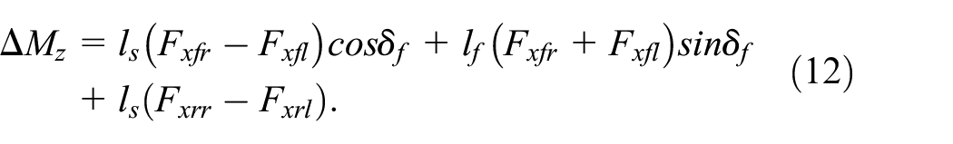
where
Path following model
Figure 3 illustrates the dynamic model of path following. X, Y coordinates represent the global coordinate system. The red solid line is the reference path.
In two-dimensional Frenet frame, the path following dynamic model 28 can be expressed as
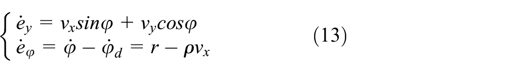
where r and

Path following dynamic model.
To achieve more stable control, the preview mechanism29,30 is introduced.

The selection of preview distance is a very crucial step in preview tracking. Vehicle speed has a significant impact on preview distance. To ensure safe driving, it is imperative to increase the preview distance as vehicle speed increases. The preview distance also decreases with a decrease in vehicle speed. However, the preview distance should be less than the maximum visual distance, which can be expressed as

where

where
Combine equations (1)–(8) with equation (10), the error dynamic model can be expressed in matrix form as

where
Controller design
It was proposed that a control strategy based on yaw stability controller and yaw angle tracking controller, can be used to deal with lumped uncertainty and maintain vehicle stability during path following. The general framework of the proposed strategy is shown in Figure 4. In real-time, the path planning module generated the reference path which provides road information to yaw angle generator. The yaw angle tracking controller, that is, the error feedback controller, was designed utilizing the sliding mode control to enhance the robustness of the system. Then, the resulting steering angle was applied to the steering actuator. In order to generate the external yaw moment, the yaw stability controller based on sliding mode control with new reaching law was deployed. Then, the moment was distributed to each tire through an optimal torque distributor. Lastly, the distributed moment was applied to the 4WID-EV.

The general framework of the path following.
Yaw angle tracking controller
The purpose of this subsection is to develop an extended state observer to observe the total disturbance. Then it can be compensated in an error feedback controller, which is designed based on a sliding mode controller.
Nonlinear extended state observer
The active disturbance rejection control (ADRC) was first proposed by Han 32 which is composed of three parts, including tracking differentiator (TD), nonlinear extended state observer (NLESO), and nonlinear state error feedback (NLSEF). The framework of traditional ADRC is shown in Figure 5. The commonly used observer in ADRC includes linear and nonlinear extended state observers. We adopted the nonlinear state observer (NLESO) in our study which is more effective in tracking precision, anti-interference capability, and response time compared with the linear state observer (LESO). During the design of NLESO, the total system disturbance is extended to a new state variable, that is, the total system disturbance, which can be estimated and compensated through the input and output quantity of the system. The designed process is as follows:
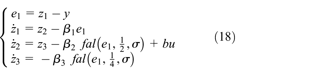
where
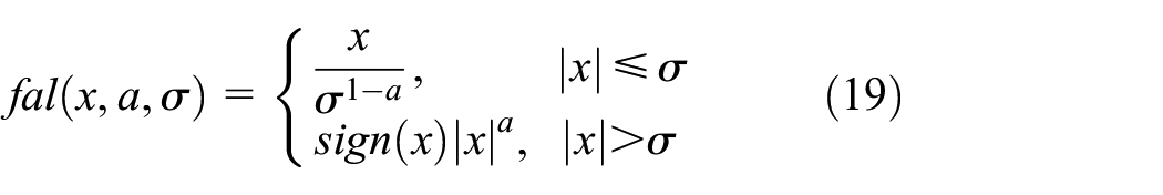
where sign( ) is the sign function.

Framework of ADRC.
Desired yaw angle
The desired yaw angle is given as 9

where
Nonsingular terminal sliding mode controller
To track the desired yaw angle, we need to design an error feedback control algorithm. Here the nonsingular terminal sliding mode control is adopted. First, the sliding surface s is given as

where
Differentiating s with respect to time yields

According to equation (9),

Therefore
Let

The reaching rate is

So the controller input of the steering angle can be expressed as
Desired yaw rate and sideslip angle
The desired yaw rate24,33 for the vehicle can be obtained from the steering angle, vehicle speed, and vehicle parameters as follows

where
Taking the tire-road condition into account, the yaw rate is limited as follows

where
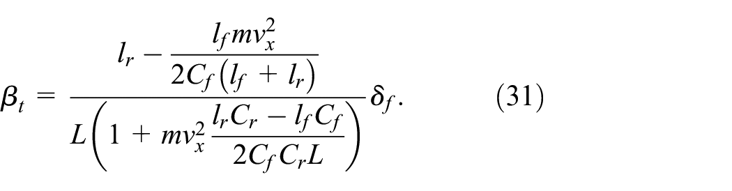
Similarly, the desired sideslip angle can be expressed as

where
Yaw stability control
In this subsection, we will design a sliding mode controller to maintain the stability of the vehicle during the path following.26,33 The object of the controller is to drive the sideslip angle and yaw rate to follow the desired sideslip angle and yaw rate. Unlike the conventional sliding mode control (SMC) method, the designed SMC will reduce the chattering problem furtherly and will be more robust to lumped disturbance. The design process includes two steps below.
Sliding surface design
The sliding surface is defined as 34
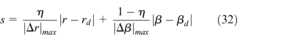
where
Reaching law design
There are many different types of reaching law that we can adopt, including exponent reaching law
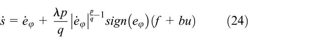
The proposed reaching law is described as 26

The derivative of sliding surface s, that is, equation (30) can be given by

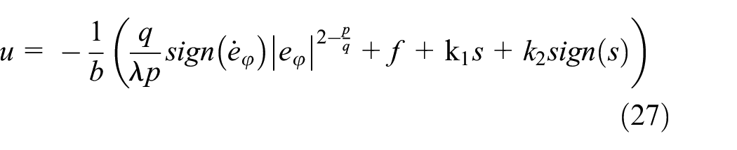
Combing equation (10) with equations (31) and (32), we obtain the following control law

where

To suppress the chattering problem, the sign function sign(s) is replaced by the hyperbolic function tanh(s).
Optimal yaw moment distribution
In what follows, we will address the problem of yaw moment distribution, that is, allocating the external yaw moment to each tire. The equation (10) can be rewritten as

where

where
Let

To obtain the optimal yaw moment distribution, we define the following cost function10,17,23,33

where
According to equation (40), we have
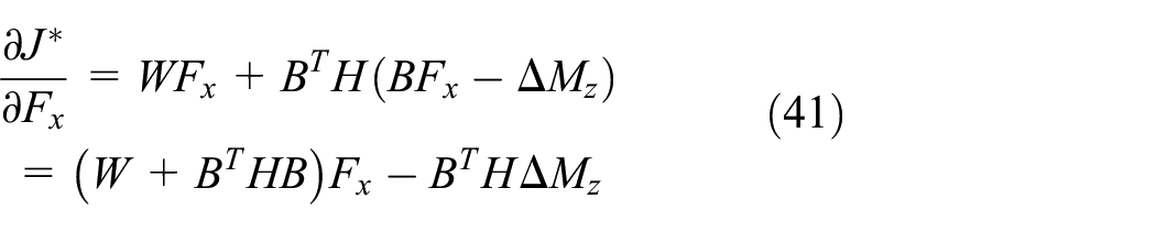
From (40), we know that if

Here, H is chosen as the identity matrix and W is designed as a function of the vertical load, proportional to the vertical load, and increases as the vertical load increases. W satisfies

where

where
Simulation and discussion
To verify the effectiveness and robustness of the proposed control strategy, the simulation is conducted on a co-simulation platform based on Matlab/Simulink and Carsim. The D-class SUV model in Carsim is adopted and the detailed vehicle parameters in simulation are listed in Table 1.
Furthermore, preview time
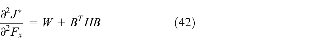
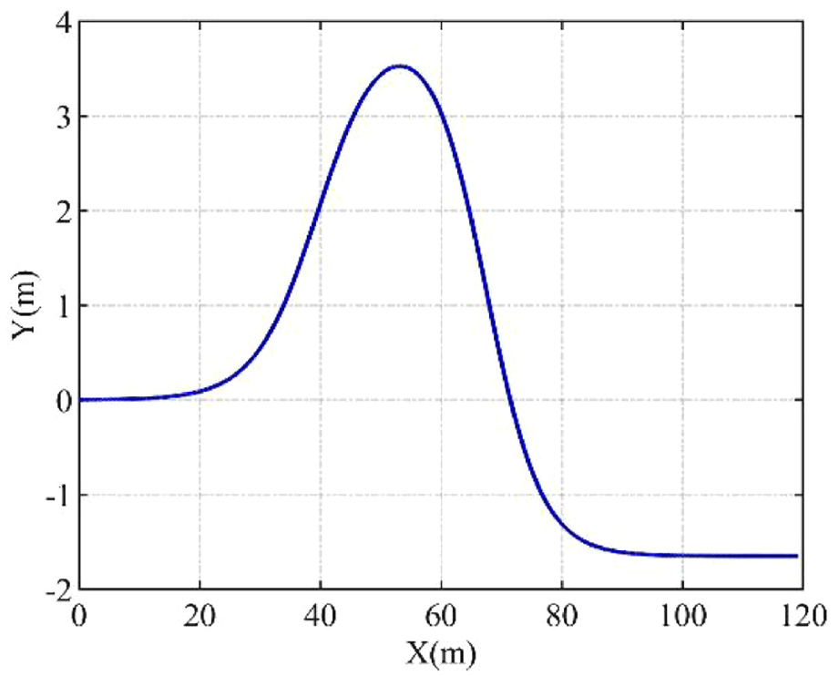
In this paper, we apply the double-lane change (DLC) maneuver in the following cases to evaluate the path-following performance. The reference path and its curvature of it are shown in Figures 6 and 7. The detailed path information can be referred to Falcone et al. 35
Reference path.
Curvature of the reference path.
In what follows, the proposed control strategy and linear quadratic regulator (LQR) are compared. For brevity, the proposed control strategy is referred to as the “ESO based.” The detailed design of the LQR controller is given in Appendix A.
Effectiveness verification
It is examined here whether the proposed control strategy is feasible and effective. First, we verify the effectiveness of preview control and moment distribution under the condition that the friction coefficient and the speed of the vehicle are 0.8 and 10 m/s, respectively. To evaluate the accuracy of different control strategies, the maximum error
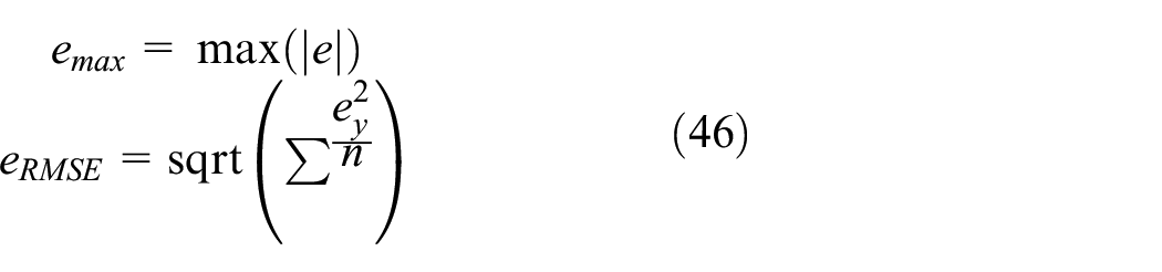
where n is the number of samples.
The path following results with and without preview control is shown in Figure 8. In the figure, it is evident that path following performance is improved with preview control compared to performance without preview control. The maximum path following error with preview and without preview control are 0.0756 and 0.0739 m, respectively. Meanwhile, the root mean square error of the two methods are 0.0317 and 0.0332, respectively.

The path following result with and without preview control.
Figure 9(a) and (b) show the simulation results of yaw moment distribution with sign function and hyperbolic tangent function, respectively. From the local enlarged drawing of Figure 9(a), we can see that transient abrupt change at the time around 7 s and chatting phenomenon at the time around 8 s occur. It is because of the introduction of the discontinuous sign function. When the sign function is replaced by the hyperbolic tangent function, the curve becomes very smooth, as shown in Figure 9(b). Furthermore, it is clear from Figure 9(b) that the moment assigned to the outer front is maximal and the moment assigned to the inner front is minimum when the vehicle is conducting the lane change maneuver.

Moment distribution results: (a) moment distribution with sign function and (b) moment distribution with hyperbolic tangent function.
In the subsequent section, the path-following performance of the vehicle under extreme conditions with different control strategies is investigated. In this case, the vehicle is made to drive at high velocity on a road with a low coefficient of friction. The velocity and coefficient of friction are set to 20 m/s and 0.4, respectively. The results in this case are illustrated in Figure 10.

The path following result with LQR and proposed control strategy: (a) path following in the X-Y plane, (b) lateral error, (c) heading angle error, (d) steering angle, (e) yaw rate, and (f) longitudinal velocity.
Figure 10(a) presents the path-following results using LQR and the proposed controller. It can be seen that the ESO-based controller can follow the reference path fairly well. However, as can also be observed, the vehicle controlled by the LQR controller initiates to drift away from the reference path and loses control at the end of the second lane change. It is clear that the proposed control strategy has superior path-following performance under extreme conditions compared to the LQR controller.
Control accuracy can be examined in terms of lateral and heading angle errors as shown in Figure 10(b) and (c). For quantitative analysis, Table 2 lists the maximum and root mean square errors of lateral distance and heading angle using two controllers. From these two indices, it is evident that the proposed control strategy provides better control compared to the LQR controller. By introducing an extended state observer, the ESO-based controller can eliminate the large model error during the lane change. As a result, both the maximum lateral and mean square errors are smaller for ESO than for the LQR controller. Figure 10(d) demonstrates the steering angle in this case using both controllers. It can be observed that the steering angle required by the ESO-based controller is significantly less than that of the LQR controller. The steering angle controlled by the LQR controller exceeds the maximum input steering angle. This means that the vehicle loses control. It can also be concluded that using ESO-based controller consumes less energy while obtaining better path-tracking performance. The yaw rate time histories for two different controllers are given in Figure 10(e). ESO-based controller keeps the yaw rate in a reasonable region, whereas LQR controller cannot maintain vehicle stability and the yaw rate occurs oscillations. Additionally, we can see that the ESO-based controller can eliminate the fluctuations dramatically. Figure 10(f) displays the time history of longitudinal velocity under the two controllers during the process of the lane change. From Figure 10(f), it can be seen that the ESO-based controller makes longitudinal velocity vary from 18.5 to 20.46 m/s, whereas longitudinal velocity controlled by the LQR controller drops sharply from 20 to 5.41 m/s. Therefore, we can conclude that the proposed control scheme has little effect on longitudinal velocity compared with the LQR method.
Comparison results of the path following.

Robustness verification
A robustness analysis of the proposed control strategy will be presented in this section. There are three different conditions which are designed to simulate. The LQR controller is used to make comparisons.
Robust to speed
As a measure of robustness to speed, we have set the vehicle speed to 10, 15, and 20 m/s, respectively, and set the friction coefficient between the tire and the road to 0.9. Figure 9 presents the simulation results under different conditions of speed. Figure 11(a)–(d) shows the path following trajectory, lateral error, heading angle error, and yaw rate, respectively.
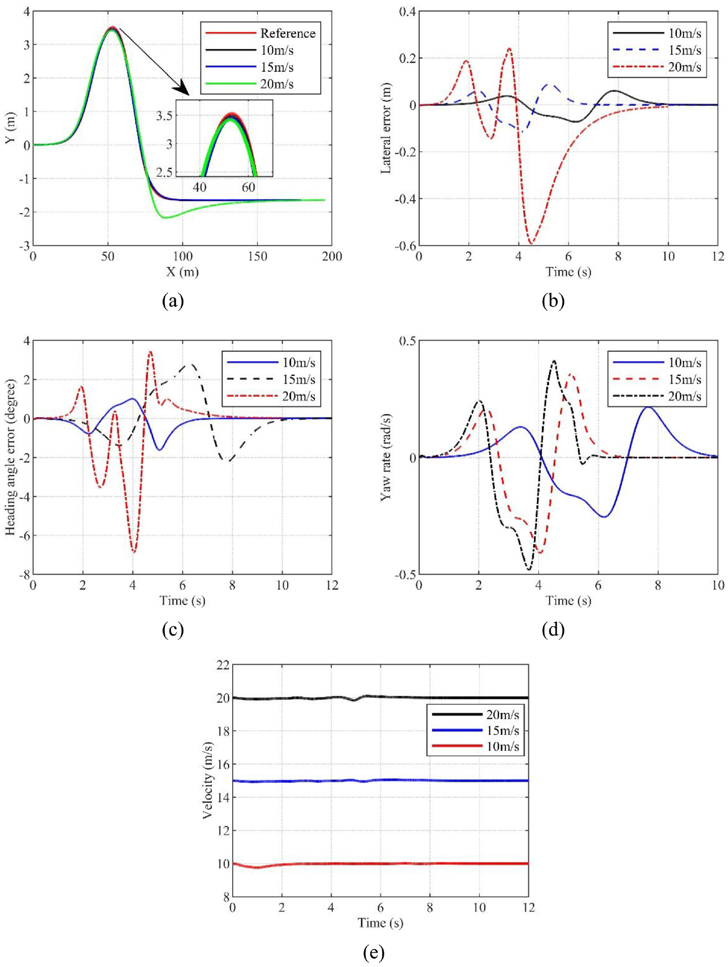
Path following performance at different speeds with ESO-based method: (a) path following trajectory, (b) lateral error, (c) heading angle error, (d) steering angle, and (e) time history of longitudinal velocity.
From Figure 11(a), we can see that the motion path of the vehicle at a speed of 10 and 15 m/s is close to the reference path. The following error reaches the maximum when it travels at a speed of 20 m/s. A lateral error increases with an increase in speed as can be observed in Figure 11(b). It means that the faster the speed, the worse the tracking accuracy. In the case of a speed of 20 m/s, the maximum error is 0.59 m. Similarly, from Figure 11(c), we can observe that the faster the speed, the larger the heading angle error. However, the heading angle error varies between 3.7° and 6.2° which is an acceptable range. From Figure 9(d), it can be found that the yaw rate is always within the limit. Therefore, the vehicle is stable during the path following process and the proposed control strategy has strong robustness to speed.
To compare the robustness of another controller, we conduct a simulation with LQR controller under the same condition. Figure 12 presents the simulation results. Figure 12(a)–(d) illustrates the moving path, lateral error, heading angle error, and yaw rate, respectively. Comparing Figure 12(a) with Figure 11(a), we can find that the path following accuracy in Figure 12(a) gets worse. Especially, when the speed is 20 m/s, the path-following accuracy is worst and the vehicle begins to lose control. As well, there is some jitter after the double lane change maneuver has been completed at speeds of 10 and 15 m/s. Similarly, we can see from Figure 12(b), the lateral error becomes very large when the vehicle travels at a speed of 20 m/s. The maximum lateral error reaches up to 7.82 m. In Figure 12(c), the heading angle error is within a reasonable range at a speed of 10 and 15 m/s. When the speed increases up to 20 m/s, the heading angle is maximum up to 20.2°. Then it starts to diverge and chatter. From Figure 12(d), the yaw rate does not converge to zero, and it diverges after the fourth second. Figure 12(e) presents the time history of longitudinal velocity. It is obvious that the proposed control strategy has little effect on the longitudinal velocity which remains unchanged.

Path following performance at different speeds with LQR method: (a) path following in X-Y plane, (b) lateral error, (c) heading angle error, and (d) yaw rate.
As a result of the above analysis, we can conclude that the vehicle is capable of following the path at different speeds with a small following error and it provides better performance than an LQR controller.
Robust to the tire-road friction coefficient
A vehicle traveling at 10 m/s is considered in this condition. Figure 5 illustrates how we test the robustness of the proposed strategy against speed by putting the vehicle on a road with varying tire-road friction coefficients, ranging from 0.8 to 0.4, and directing it to follow the reference path. The simulation results are shown in Figure 13. From Figure 13(a) and (b), it can be seen that lateral error increase with the decrease in friction coefficient. When the respective friction coefficient is 0.8, 0.6, and 0.4, the maximum lateral error is 0.0594, 0.0874, and 0.9324, respectively. Especially, the friction coefficient is 0.3, the lateral error reaches the maximum among the three cases. In addition, it is noted that when friction coefficient decreases, the convergence time of lateral error gets longer. However, the error can converge to zero in the end. A simulation result for sideslip angle and yaw rate is shown in Figure 13(c) and (d). It can be seen from the figure that the yaw rate and sideslip angle are maintained within a reasonable range. That means the proposed control strategy is robust and the vehicle is stable when the friction coefficient varies from 0.3 to 0.8. It is worth noting that when the friction coefficient is very small, such as

Path following performance using ESO-based method: (a) path following in X-Y plane, (b) lateral error, (c) sideslip angle, (d) yaw rate, and (e) longitudinal velocity.
The LQR controller is simulated under the same conditions as the ESO-based controller to assess its robustness to different tire-road friction coefficients. Figure 13 presents the simulation result. From Figure 13(a) and (b), it can be observed that the following performance is good under the high road adhesion condition. The following error is very small when the friction coefficient is 0.8 or 0.6. However, if the vehicle travels under poor road adhesion conditions, that is,

Path following performance using LQR method: (a) path following in X-Y plane, (b) lateral error, (c) sideslip angle, and (d) yaw rate.
Robust to external disturbance
Here, the vehicle runs on a high tire-road friction coefficient, that is,

The simulation results under lateral side wind disturbance: (a) side wind disturbance signal, (b) following path, (c) yaw rate, and (d) estimated total disturbance.
Conclusion
This paper deals with the issue of path following for 4-WID EV considering the lumped disturbance. The distributed control framework is adopted, which mainly consists of two relatively independent controllers. A novel control scheme based on a nonlinear state observer and sliding mode control is also proposed in this study as a solution to the path-following problem for 4WID-EV. Furthermore, the sliding mode control with modified reaching law and the optimal torque distribution method is presented to track the desired yaw rate and sideslip angle to maintain vehicle stability. Simulation experiments are conducted to assess the effectiveness and robustness of the proposed approach. According to comparison simulation results, the proposed control scheme performs better than the LQR method in terms of the following accuracy and robustness.
In addition, a few considerations should be made, including: such as the implementation of adaptive preview distance according to the state of the vehicle and path curvature, the application of the proposed control technique in a real vehicle, and the robustness of the proposed control strategy to model uncertainties. These issues are left for future study.
Footnotes
Appendix A: LQR controller design
Assume that the lumped disturbance w in equation (12) satisfies the matched condition. It is reasonable to make this assumption. The detailed explanation can be found in Hu et al. 10 So, w can be rewritten as
where
For system (14), if we don’t consider lumped disturbance term
The quadratic performance index (QPI) J with infinite time interval is defined as:
where the terminal state vector
It should be noted that the third term
The feedforward steering angle is
where R is the radius of curvature, L is the wheelbase, that is,
In this paper, the parameters for the LQR controller are as follows:
Handling Editor: Chenhui Liang
Declaration of conflicting interests
The author(s) declared no potential conflicts of interest with respect to the research, authorship, and/or publication of this article.
Funding
The author(s) disclosed receipt of the following financial support for the research, authorship, and/or publication of this article: This research was funded by University Natural Science Research Project of Anhui Province, grant number KJ2020A0507 and Natural Science Foundation of Anhui Province, grant number 1908085MC62.