
Abstract
The Weibull distribution (WD) is an important lifetime model. Due to its prime importance in modeling life data, many researchers have proposed different modifications of WD. One of the most recent modifications of WD is Modified Weibull Extension distribution (MWEM). The MWEM has been shown better in modeling lifetime data as compared to WD. However it comparison with other modifications of WD, in modeling product lifetimes and reliability, is missing in the current literature. We have attempted to bridge up this gap. The Bayesian methods have been proposed for the analysis under non-informative (uniform) and informative (gamma) priors. Since the Bayes estimates for the model parameters were not available in closed form, the Lindley’s approximation (LA) has been used for numerical solutions. Based on detailed simulation study and real life analysis, it has been concluded that Bayesian methods performed better as compared to maximum likelihood estimates (MLE) in estimating the model parameters. The MWEM performed better than eighteen other modifications of WD in modeling real datasets regarding electric and mechanical components. The reliability and entropy estimation for the said datasets has also been discussed. The estimates for parameters of MWEM were quite consistent in nature. In case of small samples, the performance of Bayes estimates under ELF and informative prior was the best. However, in case of large samples, the choice of prior and loss function did not affect the efficiency of the results to a large extend.
Introduction
The use of WD in reliability engineering is very frequent due to its flexibility in modeling the life datasets. It has increasing, decreasing, or constant hazard rate function. These kinds of models are very useful in reliability engineering while modeling the complete life cycle of a system. Due to its popularity, many researchers have introduced different modifications of this model to make it more flexible. Some valuable contributions regarding the classical and Bayesian analysis for the various modifications of the WD have been discussed in the following. Silva et al. 1 introduced five parametric lifetime distribution named as beta modified WD which was used for modeling phenomenon with monotone failure rates. Using real life dataset, the proposed model was proved to be better model as compared to exponentiated Weibull, generalized modified Weibull and modified Weibull distribution. Almalki and Yuan 2 introduced a new modified WD and obtained moment estimates and maximum likelihood estimate (MLE) using order statistics. The Bayes estimates were obtained using LA. Ahmad and Iqbal 3 proposed the generalized flexible Weibull extension distribution and compared its applicability with different conventional life models, such as flexible Weibull extension, Weibull, Rayleigh and exponential distribution. The proposed model was explored to be an appealing alternative to the competing models. El-Morshedy et al. 4 introduced three parametric exponentiated inverse flexible Weibull extension distribution and compared its performance with various modification of WD. The other recently introduced modifications of WD and their estimation can be seen from the contributions of Tahir et al., 5 Cordeiro et al., 6 Basheer, 7 Hassan et al., 8 and Afify et al. 9
The Bayesian estimation of modifications of the WD has also attracted the attention of many researchers. Kaur et al. 10 implemented the Bayesian and semi Bayesian estimation of generalized inverse WD parameters using LA. Nofal et al. 11 proposed transmuted exponentiated additive WD and estimated the concerned model parameters using classical and Bayesian methods. Similarly, the MLE and Bayesian estimation was considered for burr XII exponential distribution, 12 modified beta modified WD, 13 beta exponentiated modified Weibull distribution, 14 inverse WD, 15 exponentiated inverse Rayleigh distribution, 16 and transmuted exponentiated modified Weibull distribution. 17 The other important contributions regarding Bayesian analysis of the other models are available in the following contributions. Feroze 18 proposed Bayesian improved estimation for highly skewed data. Feroze et al. 19 considered analysis of heterogeneous datasets having detection limits via improved Bayes estimates. Feroze et al. 20 proposed Bayesian estimation for models with U-shaped hazard rate. Alshenawy et al. 21 discussed the Bayesian analysis for Burr distribution. Tung et al. 22 proposed a class of Bayes estimates for estimating a novel modification of the Weibull model. Ajmal et al. 23 considered Bayesian analysis for randomly censored samples from Weibull distribution. Chacko and Mohan 24 proposed Bayesian analysis of Weibull model under random censoring.
Many of the reliability datasets can be modeled by using a model having bathtub hazard rate function. Many authors have considered the modeling of bathtub curve. However, majority of those models are not the generalization of the Weibull model. Due to versatility of the Weibull model it can be interesting to model the bathtub-shaped hazard rate function by extension of Weibull model. The modified Weibull extension model (MWEM), proposed by Xie et al. 25 is convenient for lifetime modeling with three model parameters. In modeling the bathtub curve, the use of this model has some advantages over the other Weibull extension models. As this model has less number of parameters, the confidence interval for the shape parameter and joint confidence interval can be derived explicitly. Xie et al. 25 showed that this model can produce more efficient results, in modeling lifetime data, as compared to Weibull and exponentiated Weibull model. Yang et al. 26 considered the MWEM to estimate the reliability of satellites. The orbit lifetime dataset was used for analysis. The Bayesian approach was used for numerical estimation. Different models such as Weibull, mixed Weibull were compared with MWEM in modeling the said data. However, the MWEM was found to be the most efficient model in estimating the satellite reliability.
We have compared the performance of MWEM with eighteen other modifications of WD using different real datasets. In addition, we have conducted the detailed analysis of three-parametric MWEM under Bayesian approach. The non-informative (uniform) prior and informative (conjugate gamma) prior has been assumed for the Bayesian estimation. In addition, different loss functions such as, squared error loss function (SELF), quadratic loss function (QLF), precautionary loss function (PLF), and entropy loss function (ELF) have been used for the posterior estimation. As the posterior estimates do not have explicit forms, LA has been used for the numerical solutions. The results from the study suggest that MWEM performed better than other three to six parametric modifications of the WD. The proposed Bayes estimates for the parameters of MWEM were consistent in nature.
The rest of the article is arranged in the following sections. Section-2 contains the methods to estimate the parameters of MWEM. The numerical estimation of model parameters from MWEM and comparison of MWEM with other modifications of WD has been reported in Section-3. Finally, Section-4 concludes the article.
Methods
The probability density function (PDF) of the MWEM is

where
The cumulative distribution function (CDF) of the MWEM is

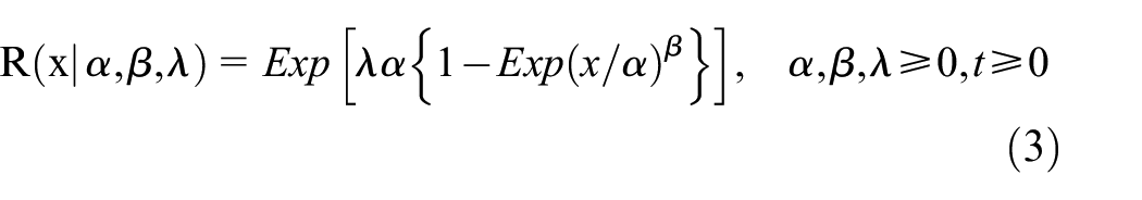
The reliability function for the MWEM is
The failure rate function for the MWEM is

The quantile function of MWEM is

where α is a scale parameter and β,
Likelihood function under complete dataset
The likelihood function for MWEM using a sample of size “n” is

Prior distributions for parameters of MWEM
The additional advantage of the Bayesian methods is that they can incorporate the prior information to update the current state of knowledge about the model parameters. This study includes the assumption of non-informative and informative priors for Bayesian estimation under different loss functions.
The joint non-informative (uniform) prior for the parameters of MWEM is:

where
The joint informative prior assuming gamma prior for each parameter of MWEM is:

where
Posterior distribution and loss functions
The posterior distribution under uniform prior

The posterior distribution under Gamma prior

As the closed form expressions for the Bayes estimates of model parameters under SELF, PLF, QLF, and ELF are not possible, the Bayesian approximate method, namely, LA has been used to obtain the numerical solutions for model parameters under the said loss functions.
The introduction of the loss functions used in the study is presented in the following.
The SELF is defined as:
Lindley’s approximation
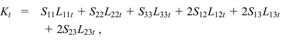
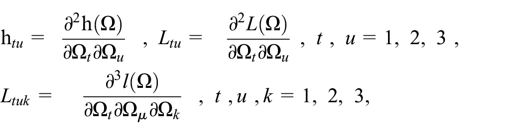
Having sufficiently large samples, Lindley 27 proposed that function of the form

where
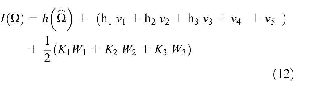
where


and
Results and discussion
This section has two main parts. The first part presents the comparison of MWEM with eighteen other modifications of WD using two real datasets. The competing modifications of the WD involve three to six parameters. The second part reports the detailed simulation study for comparing different estimates for the parameters of MWEM. The said comparison has been made between MLE and Bayes estimates using different priors and loss functions. In particular, we have assumed informative (gamma) priors and non-informative (uniform) priors for estimation of the model parameters. Additionally, the SELF, PLF, QLF, and ELF have been used for comparing estimates under Bayesian methods.
Comparison of MWEM with modifications of WD using real datasets
We have used two real datasets reported by Murthy et al. 28 dataset-1 (D1) represents the lifetimes of 20 electrical component having following observations 0.03, 0.12, 0.22, 0.35, 0.73, 0.79, 1.25, 1.41, 1.52, 1.79, 1.80, 1.94, 2.38, 2.40, 2.87, 2.99, 3.14, 3.17, 4.72, and 5.09. The dataset-2 (D2) contains the observations regarding number of shocks before failure of system. The data are 2, 3, 6, 6, 7, 9, 9, 10, 10, 11, 12, 12, 12, 13, 13, 13, 15, 16, 16, and 18. The summary statistics for these data have been given in Table 1.
Description of real datasets.

The goodness-of-fit results for MWEM using the real datasets and estimates of the parameters of MWEM, -2log-likelihood value, AIC, BIC K-S, and p-value, have been given in Table 2. From this table, it can be seen that MWEM fits both datasets efficiently. The p-values for goodness of fit using K–S test are 0.8 and 0.96, respectively, which reveals that the fits are quite good.
Goodness of fit for MWEM using different real data sets.

D i denotes ith real dataset.
The modeling capability of the proposed model has been compared with different modifications of WD. These modification include Weibull Extended Generalized Exponential Distribution (WEGED), Weibull Extended Generalized Rayleigh Distribution (WEGRD), Weibull Extended Generalized Weibull Distribution (WEGWD), Weibull Extended Generalized Gamma Distribution (WEGGD), Weibull Extended Generalized lognormal Distribution (WEGLND), Weibull Extended Generalized Burr XII Distribution (WEGBXIID), Weibull Extended Generalized Chi-square Distribution (WEGCSD), Weibull Extended Generalized Frechet Distribution (WEGFD), Weibull Extended Generalized Gompertz Distribution (WEGGOD), Weibull Extended Generalized Log-Frechet Distribution (WEGLFD), Weibull Extended Generalized Lomax Distribution (WEGDLOD), Weibull Extended Generalized Log-Logistic Distribution (WEGLLD), Exponentiated Weibull Distribution (EWD), Beta Extended G Weibull Distribution (BEGWD), Exponentiated Kumaraswamy Weibull Distribution (EKWD), Exponentiated Generalized Weibull Distribution (EGWD), Gamma GI Weibull Distribution (GGIWD), and Gamma GII Weibull Distribution (GGIIWD). Tables 3 and 4 represent the comparison of MWEM with eighteen other modifications of the WD, having three to six parameters. From these tables, it can be accessed that the fits under MWEM are better than those under other modifications of the WD for both datasets. Hence, the MWEM is a promising alternative candidate to various complex modifications of WD in modeling different lifetime data sets.
Comparison of MWEM with different modifications of WD using D1.

Comparison of MWEM with different modifications of WD using D2.

The amounts of MSEs associated with estimates under MLE and Bayesian methods, using D1 and D2, have been presented in Figures 1 and 2, respectively. These figures elucidate that all the estimation methods have provided satisfactory estimates. However, the estimates under ELF are slightly better than those under MLE, SELF, QLF, and PLF.
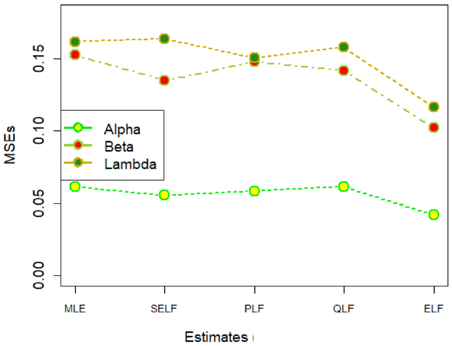
MSEs for estimates using real dataset-1.

MSEs for estimates using dataset-2.
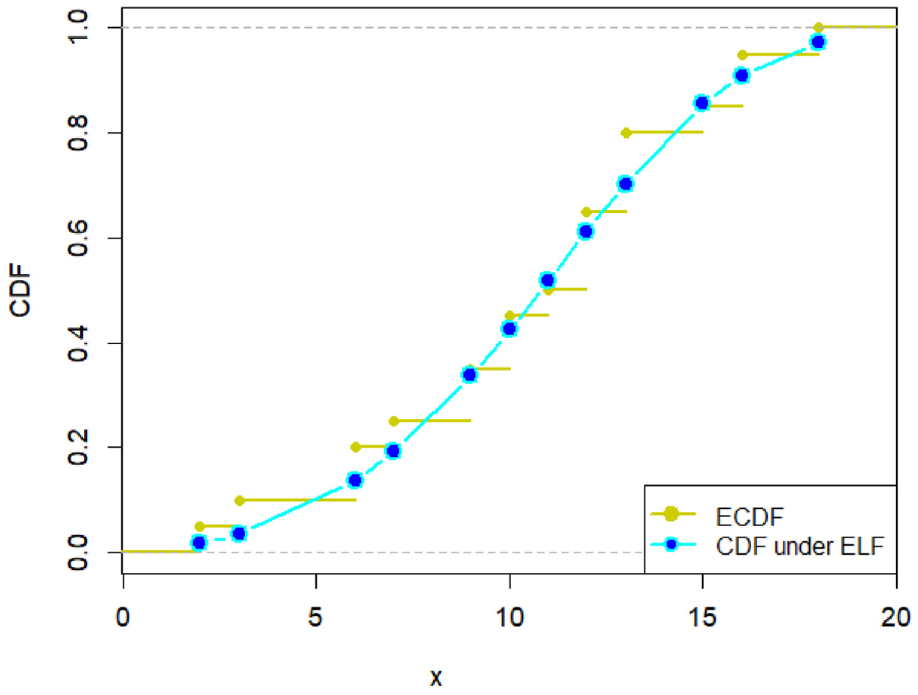
Since the estimation under ELF outperformed its counterparts, we have reported the description of estimates under ELF in detail. For that purpose, the density plots and CDF plots for both real datasets have been reported in Figures 3–6, respectively. These figures indicate that the estimates under ELF have been quite efficient in describing the behavior of each real datasets. This is due to the fact that estimated density curves and CDF curves, under ELF, are quite closer to the corresponding empirical curves.

Density curve for uncensored real D1.

CDF plot for D1 using estimates under ELF.

Density curve for uncensored real D2.
CDF plot for D2 using estimates under ELF.
Reliability estimation from MWEM
The reliability plots, under different estimation methods MLE and Bayes have been reported in Figures 7 and 8. These figures have been obtained using D1 and D2 respectively. The reliability curves under proposed estimates have been compared to those under Kaplan-Meier method. From the represented figures, it can be seen that reliability curves under ELF are closer to the empirical reliability curves, especially in case of D2. Hence the proposed estimator under ELF can be efficiently used to study reliability of products using MWEM.
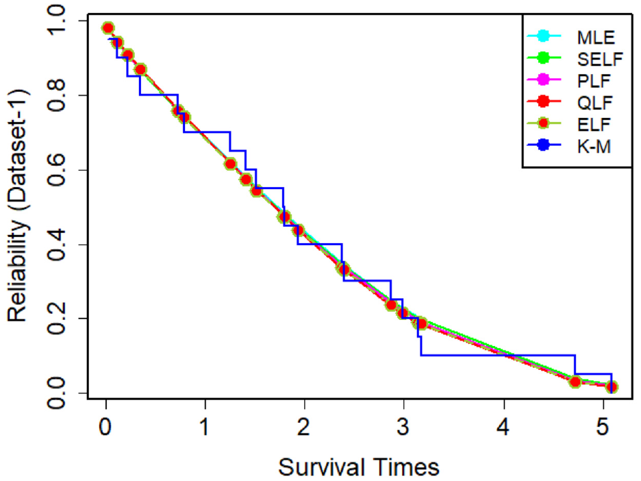
Reliability plot for uncensored real D1.

Reliability plot for uncensored real D2.
Entropy estimation for MWEM
This section contains the entropy estimation for MWEM using D1 and D2, respectively. Here we estimate only two types of entropy namely Shannon’s entropy and Renyi’s entropy and also find Gini index and presented the Lorenz curves for MWEM.
The Shannon entropy and Renyi entropy are used to measure the diversity in the systems. The results for Shannon’s and Renyi’s entries using real datasets have been reported in Table 5. From the results it can be assessed that the diversity in D2 is lower than D1. The pattern is similar both under Shannon’s and Renyi’s entropy. The result for the Gini index has also been placed in the Table 5. The results for Gini index are again relatively lower for D2 as compared to D1.
Entropy estimation from MWEM using different real datasets.

The Lorenz curves for D2, given in Figure 9, has less difference from the baseline curves, suggesting the less inequality of the observation in data. On the other hand, the Lorenz curve for D1, given in Figure 10, exhibit more spread from the respective baseline curves suggesting slightly increase inequality in the distribution of data.

Lorenz curve for MWEM using D2.

Lorenz curve for MWEM using D1.
Simulation study
This section contains the simulation study for the proposed Bayes estimates and MLEs using different sample size, different parametric values, different loss functions, under informative prior (I.P) and non-informative prior (N.I.P). Tables A1–A9, given in appendix, reports the estimates for the parameters of MWEM using different simulated datasets. The graphs for amounts of mean square errors (MSEs) associated with estimates using simulated datasets of size n = 20 and 100 for different parametric values, have been placed in Figures 11 to 19. In the said figures,

MSEs using α = 1, β = 1, and λ = 1.

MSEs using α = 1, β = 2, and λ = 1.

MSEs using α = 1, β = 2, and λ = 2.

MSEs using α = 2, β = 2, and λ = 1.
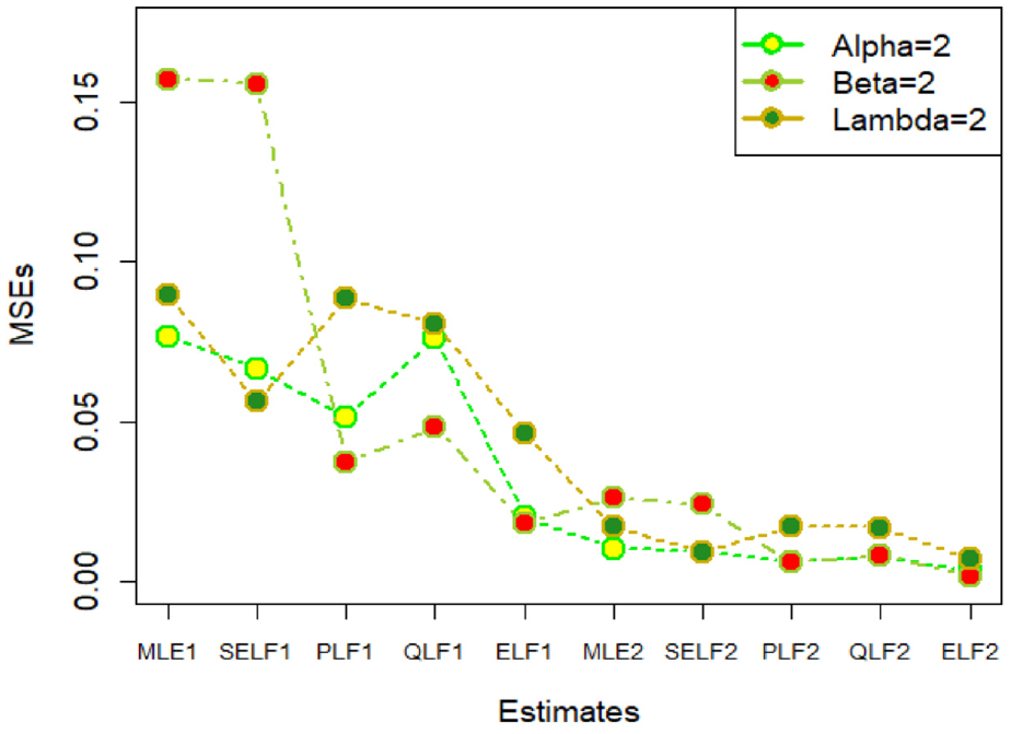
MSEs using α = 2, β = 2, and λ = 2.

MSEs using α = 0.1, β = 0.5, and λ = 0.1.

MSEs using α = 0.1, β = 0.5, and λ = 0.5.

MSEs using α = 0.5, β = 0.5, and λ = 0.1.

MSEs using α = 0.5, β = 0.5, and λ = 0.5.
The detailed comparison among different estimates has been reported in Tables A1–A9, given in Appendix. The amounts of MSEs have been presented in the bold fonts. The estimate with lower values of MSEs is considered a better estimate. In particular, the comparison between MLE and Bayesian estimation has been considered. Additionally, in case of Bayesian inference the estimates have been compared with respect to (i) informative and non-informative priors (ii) different loss functions. The detailed comparison has been carried out using different sample sizes and various parametric values. In case of informative prior, the values of hyper-parameters have been chosen using prior mean approach. The prior mean approach chooses the values for hyper-parameters in such a way that the prior mean becomes equal to the assumed true value of the parameters.
The results from the analysis suggest that Bayes estimates performed better than MLE especially in small samples, as the amounts of MSEs associated with estimates under Bayesian inference are smaller than those under MLEs. On the other hand, in case of Bayes estimates, the estimates under informative prior are better than those under non- informative prior. Further, the estimates under ELF are better than those under SELF, PLF, and QLF for (i) each sample size, (ii) each parametric set, and (iii) under both priors. Hence, the performance of estimates under ELF assuming informative prior is superior to their counter parts.
Conclusion
The study has been conducted to analyze the recently introduced MWEM using Bayesian approach. The applicability of the model has been compared with other modification of WD using two real datasets. The detailed simulation studies have been carried out using different datasets. The simulated datasets have been generated using different sample sizes and various true parametric values. Based on the simulated datasets, the comparison between MLEs and Bayes estimates has been made. This comparison is based on amounts of MSEs, AICs, BICs, K–S statistics, and corresponding p-values. In case of Bayesian estimation, the comparison among different Bayes estimates has been considered with respect to different priors Informative and Non-Informative and using four loss functions namely SELF, PLF, QLF, and ELF. Since the closed form Bayes estimates were not possible, LA was used to obtain the numerical solution. Based on detailed analysis, the study reached the following conclusions.
The comparison of Bayesian estimation with MLE suggested the better performance of the Bayes estimators, especially in smaller sample sizes (n ≤ 20). The proposed estimators are also consistent in nature.
In comparison of prior information it has been observed that the results under informative priors were slightly better than those under non-informative priors. However, the difference in the results under non-informative and informative priors was not drastic in large samples. Hence, the proposed estimators are quite insensitive with respect to change in the prior information, especially in large samples. As far as the comparison of loss functions is concerned, the Bayes estimates were superior under ELF as compared to their counterparts.
The comparison of MWEM with eighteen other modifications of the WD based on two real datasets suggested that the MWEM is superior to its counterparts in modeling these data.
The Shannon’s and Renyi’s entropies suggested that diversity is low in dataset-2 as compared to dataset-1. It was interesting to observe that the performance of MWEM was comparatively better for datasets with lower diversity. The reliability estimation from MWEM has also been considered using real datasets. The estimates based on ELF were better able to represent the behavior of reliability curves.
The study has explored the MWEM as an appealing alternative to WD and its modifications in modeling life data. The study will be useful for the researchers dealing with lifetime data needing more flexibility in modeling.
Footnotes
Appendix
MLEs, BEs, and MSEs (in bold fonts) for using complete data for α = 1, β = 1, and λ = 1.

| I.P | N.I.P | |||||||||
|---|---|---|---|---|---|---|---|---|---|---|
| n | MLE | SELF | PLF | QLF | ELF | SELF | PLF | QLF | ELF | |
| 20 | α | 1.0767 | 1.1762 | 1.1079 | 1.1039 | 1.0750 | 1.1591 | 1.2279 | 1.2688 | 1.1511 |
|
|
|
|
|
|
|
|
|
|
||
| β | 1.1088 | 1.1374 | 1.1213 | 1.1181 | 1.0778 | 1.1652 | 1.1560 | 1.1347 | 1.1295 | |
|
|
|
|
|
|
|
|
|
|
||
| λ | 1.1432 | 1.1586 | 1.1712 | 1.1788 | 1.0710 | 1.3158 | 0.9502 | 1.3019 | 1.2008 | |
|
|
|
|
|
|
|
|
|
|
||
| 50 | α | 1.0698 | 1.1564 | 1.0928 | 1.0966 | 1.0437 | 1.0829 | 1.2158 | 1.1890 | 1.0455 |
|
|
|
|
|
|
|
|
|
|
||
| β | 1.0698 | 1.1209 | 1.1182 | 1.0693 | 1.0469 | 1.0872 | 1.1026 | 1.1253 | 1.0550 | |
|
|
|
|
|
|
|
|
|
|
||
| λ | 1.0674 | 1.1264 | 1.1278 | 1.1251 | 1.0505 | 1.1633 | 1.0320 | 1.1985 | 1.1048 | |
|
|
|
|
|
|
|
|
|
|
||
| 70 | α | 1.0160 | 1.1233 | 1.0816 | 1.0744 | 1.0383 | 1.0370 | 1.1287 | 1.1116 | 1.0336 |
|
|
|
|
|
|
|
|
|
|
||
| β | 1.0393 | 1.1085 | 1.1039 | 1.0525 | 1.0278 | 1.0539 | 1.1006 | 1.1120 | 1.0438 | |
|
|
|
|
|
|
|
|
|
|
||
| λ | 1.0445 | 1.1257 | 1.0635 | 1.1202 | 1.0219 | 1.1339 | 1.1140 | 1.0773 | 1.1318 | |
|
|
|
|
|
|
|
|
|
|
||
| 100 | α | 0.9730 | 1.0776 | 1.0751 | 1.0357 | 1.0352 | 1.0186 | 1.0640 | 1.0772 | 0.9997 |
|
|
|
|
|
|
|
|
|
|
||
| β | 0.9536 | 1.0746 | 1.0362 | 1.0452 | 1.0223 | 0.9679 | 1.0714 | 1.0376 | 1.0448 | |
|
|
|
|
|
|
|
|
|
|
||
| λ | 1.0313 | 1.0467 | 1.0283 | 1.0438 | 1.0052 | 1.1046 | 1.0518 | 1.0458 | 1.0788 | |
|
|
|
|
|
|
|
|
|
|
||
Handling Editor: Chenhui Liang
Declaration of conflicting interests
The author(s) declared no potential conflicts of interest with respect to the research, authorship, and/or publication of this article.
Funding
The author(s) disclosed receipt of the following financial support for the research, authorship, and/or publication of this article This work was supported by the Deanship of Scientific Research, Vice Presidency for Graduate Studies and Scientific Research, King Faisal University, Saudi Arabia [Project No. 531].