Sage Journals: Discover world-class research

Abstract

To address the problem of low prediction accuracy in the current research on fatigue crack propagation prediction, a prediction method of fatigue crack propagation based on a dynamic Bayesian network is proposed in this paper. The Paris Law of crack propagation and the extended finite element method (XFEM) are combined to establish the state equation of crack propagation. The uncertain factors of crack propagation are analyzed, and the prediction model of fatigue crack propagation based on the dynamic Bayesian network is constructed. A Bayesian inference algorithm based on the combination of Gaussian particle filter and firefly algorithm is proposed. The fatigue experiment of the specimen with the pre-cracks is carried out to test the correlation between the fatigue load cycles and the crack propagation depth. The experimental results show that the crack propagation prediction method proposed in this paper can effectively improve the prediction accuracy of crack propagation depth.

Keywords

Fatigue crack propagation dynamic Bayesian network Gaussian particle filter firefly algorithm the extended finite element method

Introduction

Fatigue crack is one of the common damages that occur in metal structures under the fatigue loads and variable environmental factors over a long period,¹ and cracks propagation is an important factor leading to structural failure. Therefore, it is of great significance to study the accurate prediction method of fatigue crack propagation to ensure structural safety. Due to the accuracy error of the acquisition equipment and the influence of random factors in the equipment manufacturing process, the monitoring data and expansion model during the process of fatigue crack propagation is uncertain. Therefore, to improve the prediction accuracy of crack propagation, the first consideration is the integration of uncertainty factors. The traditional prediction methods of fatigue crack propagation are mainly based on theoretical and numerical methods. The theoretical method mainly integrates uncertain factors to improve the prediction accuracy by modifying the Paris Law,² there is an example of modifying the Paris Law.³ The numerical methods mainly improve prediction accuracy by using surrogate models and optimizing damage parameters. For example, there is an example about the numerical methods improving the prediction accuracy.⁴ To reasonably quantify the dynamic change characteristics of uncertainty during fatigue crack propagation, the modeling process of traditional prediction methods of fatigue crack propagation is often complicated, which reduces the applicability in practical engineering applications.

To simplify the prediction model of crack propagation and reasonably integrate the uncertainties in the crack propagation process, it is of great significance to study a new prediction method of crack propagation. As a directed acyclic graph describing the dependencies between data variables, the dynamic Bayesian network can effectively integrate real-time monitoring data with physical models, and infer and update random nodes by inputting observation data to eliminate the influence of uncertain factors.⁵ Many researchers have carried out a lot of research on the fusion of a dynamic Bayesian network and physical model for probabilistic prediction of structural damage.^6–9The particle filtering algorithm, as an inference algorithm of the Bayesian network, is a powerful tool to deal with prediction problems affected by uncertainties. In recent years, it has been widely used in remaining life prediction, crack propagation prediction and other fields. The standard particle filtering algorithm suffers from the phenomenon of particle diversity scarcity, which affects the prediction accuracy.^10,11Therefore, the improvement of the resampling and the importance sampling method in particle filtering algorithm has become a research hotspot for researchers. Studies presented in Refs^12,13 are similar to the ones shown in this paper.

In summary, the existing fatigue crack propagation has two main problems: (1) Most researchers simplify the prediction model in a mathematical model to improve computational efficiency. This simplified method can improve the computational speed of the prediction model, but also has some influence on the prediction accuracy. There is some research on the use of a dynamic Bayesian network for health monitoring and fatigue crack propagation, but there is less research on how to use the finite element model for rapid prediction of crack propagation under the framework of the dynamic Bayesian network. (2) The improvement of the particle filtering algorithm is less combined with the actual measurement value, and the problem of lack of particle diversity has not been fully solved.

To address the above problems, a prediction method of crack propagation using a finite element model for fast computation under the framework of the dynamic Bayesian network is proposed. The finite element model is simplified by using the dimensionality reduction method and the local mesh coarse-graining method to achieve an efficient prediction of crack propagation, and the dynamic Bayesian network is used to integrate the uncertain factors in the crack propagation process. On this basis, an optimized Gaussian particle filtering algorithm is proposed to improve the accuracy of prediction. Finally, the proposed method is validated experimentally, and the high-efficiency and high-precision prediction of crack propagation is achieved. Meanwhile, the optimization results of the proposed method are compared with those from the conventional Gaussian particle filtering algorithm.

The simplification methods of the finite element model

The traditional finite element method requires fine mesh algorithms and different failure criteria to accurately predict local failure behaviors, and this might result in the reduction of computational efficiency. The extended finite element method can overcome this limitation and can accurately predict the local stress field and stress concentration field without refining the mesh, so it has an advantage in fatigue crack simulation research.¹⁴ The model of fatigue crack propagation studied in this paper is based on the Paris Law. In Abaqus, the crack propagation rate is related to the energy release rate, and the energy release rate and the parameters of the Paris Law can be converted. The finite element model discussed in this study is shown in Figure 1. The finite element model is a metal plate with a length of 400 mm, a width of 80 mm, and a thickness of 8 mm, and the initial crack length is 28 mm.

Figure 1.

Schematic diagram of the study object containing pre-cracks.

To ensure the accuracy of the simulation results of the finite element model, mesh convergence is studied, and a convergence study of the crack length-load cycles curve with the mesh size has been done in this paper. As the mesh density increases, the numerical results produced by the simulation analysis may tend toward a unique solution, but the computer resources required to run the model also increase. When the change in the solution obtained by further subdivision of the mesh is negligible, the mesh has converged. In this paper, the study is carried out for the refining area. The mesh is divided into five different types 10 × 10 mm, 5 × 5 mm, 2 × 2 mm, 1 × 1 mm, and 0.5 × 0.5 mm, and the magnitude of the tip stress and the number of load cycles at the crack propagation up to 10 mm is studied, and the convergence is judged by comparing the magnitude of the tip stress and the number of load cycles.

By analyzing the data in Table 1, it can be obtained that the finite element mesh size at the first four lengths continues to grow in the tip stress at the crack propagation up to 10 mm and does not reach the convergence state, and the number of load cycles for crack propagation to 10 mm has been decreasing and has not reached a convergent state. In the fifth length, when the finite element mesh is divided into 0.5 × 0.5 mm, the stress at the crack tip grows only less than 10 MPa and the number of load cycles has been reduced by only 256 cycles, which is a significant decrease compared with the first four lengths, indicating that the finite element mesh size and the effect of mesh size on the crack length-load cycles curve has converged at 0.5 × 0.5 mm. However, if the finite element mesh is divided into 0.5 × 0.5 mm, the number of finite element mesh in the local refinement region will be four times more than that in the 1 × 1 mm case, and the computational efficiency will be greatly reduced, while the tip stress magnitude and the number of load cycles at 1 × 1 mm is only changed less than 2% compared with 0.5 × 0.5 mm, which is a small change. Considering the computational efficiency and accuracy, the finite element mesh size of 1 × 1 mm is chosen for meshing the refining area.

Table 1.

The magnitude of the tip stress under different finite element meshes.

Unit finite element mesh size/mm	10 × 10	5 × 5	2 × 2	1 × 1	0.5 × 0.5
Crack propagation to 10 mm tip stress/MPa	276.9	432.3	626.4	804.4	813.2
Crack propagation to 10 mm load cycles/numbers	45,000	38,107	31,346	22,095	21,839

To further improve the computational efficiency of the finite element model, the dimensionality reduction method¹⁵ and local mesh coarse-grained method¹⁶ are used to simplify the finite element model, as shown in Figure 2. The element type of the finite element mesh is CPS4R. The number of nodes in the coarse-grained region is 559 and the number of elements is 496; the number of nodes in the fine-grained region is 2430 and the number of elements is 2320. In this paper, the incremental step is 0.02 and the maximum number of iterations is 1. For every 50 incremental steps, the crack is propagated one mesh size forward. Therefore, for each calculation, the increment of the crack length is constant, which is the length of one mesh, and the change is the calculated number of load cycles. The feasibility of the simplified method is verified by the amount of change in stress at the crack tip and the amount of change in the number of load cycles of crack propagation before and after simplification, as shown in Figures 3 and 4.

Figure 2.

The simplification of the finite element model.

Figure 3.

Changes in stress contours before and after the dimensionality reduction method: (a) stress contour before dimensionality reduction and (b) stress contour after dimensionality reduction.

Figure 4.

Changes of stress contours before and after local mesh coarse-grained method: (a) stress contour before mesh coarsening and (b) stress contour after mesh coarsening.

From Figure 3, it can be seen that after using the dimensionality reduction method, the error of the tip stress of the model after dimensionality reduction is 1.25% compared to the 3D model. In terms of the number of load cycles required for crack propagation by 1 mm, 9889 load cycles are required for the 3D model and 9795 load cycles are required for the model after dimensionality reduction, and the error of the simplified model is 0.951%. As can be seen from Figure 4, on the basis of dimensionality reduction, the error of the tip stress after using the coarse-grained mesh method is 0.252%. In terms of the number of load cycles required for the crack to propagate 3 mm, 17,564 load cycles are required for the full fine-mesh model and 17,553 load cycles are required for the partial coarse-grained mesh model, and the error of the model after the partial coarse-grained mesh is 0.0626%. The comparison of the model operation speed after using the simplified method is shown in Table 2.

Table 2.

Fusion effect of multiple simplification methods.

	3D full-order model	Dimensionality reduction	Dimensionality reduction and local mesh coarsening
The simulation time of 800 incremental steps	96 min	6.5 min	3.2 min
The error of simplification result	0	0.95%	1.28%

As can be seen from Table 2, the time of running 800 incremental steps of the simulation model is used as the total simulation time. The running time of the 3D full-order model is 96 min, and the simulation model after using the dimension reduction method takes 6.5 min, which shortens the simulation time to 6.77% of the original one. Based on the simulation model after using the dimension reduction and local mesh coarsening, the simplified model using the local mesh coarsening methods takes 3.2 min, which is reduced to 49.36% of the running time of the original model. On the whole, after the integration of the simplified method, the simulation time of the simplified model is shortened to 3.33% of the full-order model, and the error is 1.28% compared to the full-order model.

The dynamic Bayesian network for crack propagation

To establish a dynamic Bayesian network for crack propagation, the uncertain factors in the process of crack propagation are firstly analyzed, and then the dynamic variables are selected based on the simplified model of the finite element. Based on the selected dynamic variables, a dynamic Bayesian network suitable for this paper is established.

Analysis of uncertain factors

To establish a dynamic Bayesian network for fatigue crack propagation, the uncertain parameters in the model should be determined,¹⁷ and the uncertain factors considered in this paper are mainly as follow.

Uncertainties of measurement data. The dynamic Bayesian network needs real-time information collected by sensors and measurement equipment to drive the update, so there are measurement errors caused by the accuracy of the collection equipment. It is assumed that the measured value of crack length obeys a normal distribution, the mean value is the real crack length of this measurement, and the standard deviation is determined by the accuracy of the measurement tool.

Uncertainties of the model. Due to the influence of random factors in the manufacturing process of the equipment, different fatigue characteristics exist in the same group of equipment due to the geometric errors and initial defects, this affects the calculation of fatigue crack propagation. Therefore, the properties of the crack propagation model are uncertain. It is assumed that some material parameters in the crack propagation obey uniform distribution.

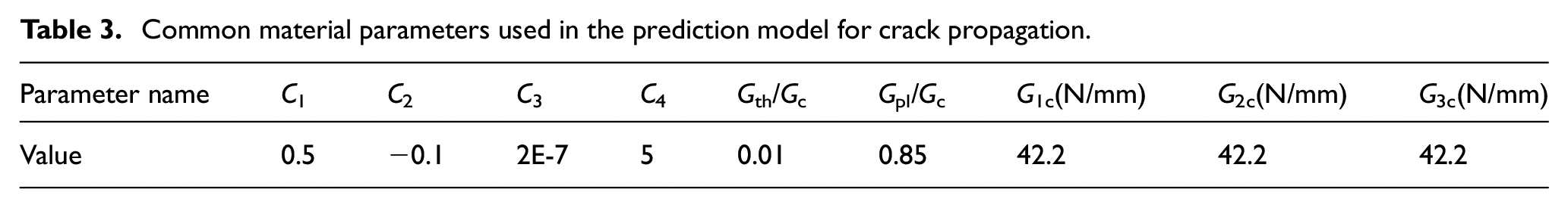
In this paper, based on XFEM of Abaqus software, the finite element model of fatigue crack propagation is established and sensitivity analysis is performed for each uncertain parameter. The optional parameters are as follows: peak cyclic load P, crack measurement length L, crack propagation influencing parameters C₁, C₂, C₃, C₄, the threshold of strain energy release rate G_th, the upper limit of strain energy release rate G_pl, critical equivalent strain energy release rate G_c, the strain energy release rates G_1c, G_2c, G_3c of the material when fractured in three directions. In this paper, it is assumed that each material simulation parameter is independent of the other. The values of G_th/G_c and G_pl/G_C are the default values set in Abaqus, and the values of C and m can be obtained by consulting the literature.¹⁸ According to the literature review^19,20 and simulation calculation, the initial setting values of parameters C₁, C₂, G_1c, G_2c, and G_3c are obtained, respectively, used as prior parameter values. C₃ and C₄ need to be converted by the parameters C and m of the Paris Law.¹⁹

Since parameters G_th, G_pl, G_c, G_1c, G_2c, G_3c does not support the fatigue analysis changes in this case study or their values do not affect the crack propagation itself, the parameters are not presented as a dynamic variable in this paper, but only as a standard parameter used for modeling. In this paper, parameters C₃, C₄, P, L are set as a variable parameter for research. The initial material parameters of the simulation model are obtained as shown in Table 3.

Table 3.

Common material parameters used in the prediction model for crack propagation.

Parameter name	C ₁	C ₂	C ₃	C ₄	G _th/G_c	G _pl/G_c	G _1c(N/mm)	G _2c(N/mm)	G _3c(N/mm)
Value	0.5	−0.1	2E-7	5	0.01	0.85	42.2	42.2	42.2

The magnitude of change in simulation results is analyzed based on the control variable method to determine the sensitivities of each parameter. The analysis of parameter sensitivities requires the selected initial parameter values to fluctuate up and down to test the degree of influence of the parameter on crack propagation. The parameters are defined as high-sensitivity and low-sensitivity parameters according to the magnitude of the influence. To improve the simulation efficiency and better show the floating range of the high-sensitivity parameters, the most significant variation range of 2% is obtained by simulation analysis. The parameter values of individual variables are reduced and increased by 2%, and the number of cycles of load required for crack propagation by 1 mm is taken as a result to analyze the degree of influence of parameter value changes on the results. The results of the sensitivities analysis are shown in Table 4.

Table 4.

Comparison of parameter sensitivities.

Parameter name	Parameter value (%)	The magnitude of positive change (%)	The magnitude of negative change (%)
P (MPa)	90 ± 2	+22.39	−17.96
L (mm)	28 ± 2	+37.9	−34.6
C ₃	2E-7 ± 2	+2.04	−1.96
C ₄	5 ± 2	+11.5	−10.1

From the above table, it can be seen that the cyclic load peak P, the crack measurement length L, and the simulation material parameters C₃ and C₄ have the obvious variation range and are defined as high-sensitive parameters. The crack measurement length can be used as a high-sensitive parameter in terms of the amplitude of change in the number of cyclic loads. However, since the crack measurement instrument used in this paper is a crack gauge with an error of 0.01 mm, the crack propagation length studied in this paper is between 2 and 4 mm. The degree of uncertainty caused by the crack measurement error is estimated to be less than 0.5%, so the parameter of crack measurement length L is not suitable as a variable parameter. In summary, the cyclic load peak P and the simulation material parameters C₃ and C₄ are selected as dynamic variables with uncertainty.

Construction of the dynamic Bayesian network

Based on the dynamic variables and the Bayesian network, a model of fatigue crack propagation is constructed. The dynamic Bayesian network for the crack propagation analysis is shown in Figure 5, where P is the cyclic load, ΔL is the change of the crack state, L is the state after crack propagation, θ is the set of material parameters including C₃ and C₄, L₀ is the initial crack length, L^obs is the real-time crack length, and the subscripts t and t-1 are the current time step and the previous time step, respectively. The directed edges of the solid line represent the functional relationship between variables in the same Bayesian network, and the directed edges of the dashed line represent the functional relationship between two adjacent time-step Bayesian network state variables. The rectangular node is a function node, and the value of this variable can be obtained by deterministic computation. The elliptical node is a variable node and the directed edge pointing to it represents a conditional probability density function. The inverted triangle is the observed value input node. The dynamic Bayesian network consists of two main components.

Time step: In the time step t-1, P_t-1 and θ_t-1 are highly sensitive uncertain dynamic variables, which are input into the simulation model and are predicted by crack propagation to yield $Δ L_{t - 1}$ , while $L_{t - 1} = Δ L_{t - 1} + L_{t - 1}^{0}$ .

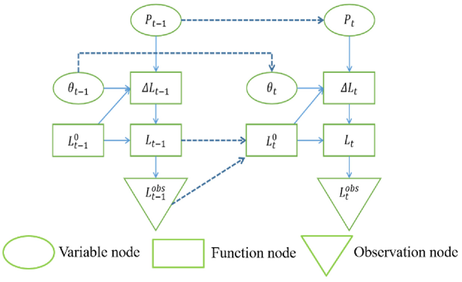
Prediction step: In the prediction step t, $L_{t}^{0} = L_{t - 1}$ , while in the diagnosis step, the observation error is ignored due to the small error of the crack width meter, and $L_{t}^{0} = L_{t - 1}^{obs}$ . If the actual value of crack length is input at time step t-1, then the prior distribution of P_t and θ_t in time step t is the previous time step t-1 parameters by Bayesian inference of the posterior distribution after the algorithm is updated.

Figure 5.

The dynamic Bayesian network for crack propagation.

Bayesian inference based on optimized Gaussian particle filtering algorithm

According to the established dynamic Bayesian network, the state equation of fatigue crack propagation is firstly derived, and then an appropriate Bayesian inference algorithm is selected based on the state equation. In this paper, the Gaussian particle filtering algorithm is optimized to further improve the accuracy of Bayesian inference.

Equation of state for fatigue crack propagation

In this paper, the fatigue crack propagation equation is as follow¹⁹:

\frac{dL}{dN} = C_{3} {(\frac{Δ K^{2}}{E})}^{C_{4}}

(1)

where L is the crack length, N is the number of load cycles, ΔK is the range of stress intensity factors, and E is the modulus of elasticity.

Thus, the relationship of the state transfer function of the crack between adjacent time steps can be obtained as follows.

L_{t} = L_{t - 1} + \frac{dL}{dN} Δ N

(2)

Where $\frac{dL}{dN} Δ N$ is the crack propagation length after one load cycle, corresponding to ΔL on the dynamic Bayesian network, which can be obtained directly from the simulation model, so the state transfer equation can be abbreviated as :

L_{t} = Δ L_{t} + L_{t}^{0}

(3)

From the above analysis, it can be seen that the error caused by the crack length measurement is negligible, so the measurement equation can be obtained as:

D_{t} = L_{t}

(4)

Gaussian particle filtering algorithm

A set of random particles are used in the particle filtering algorithm to approximate any form of probability density distribution, which can represent a wider distribution than the Gaussian model. However, a discrete approximation method to sample particles, and such a sampling method will reduce the diversity of particles to a certain extent. In contrast to the particle filtering algorithm, Gaussian density estimation is used as a continuous approximation rather than a discrete approximation to sample particles. Therefore, the Gaussian particle filtering algorithm is selected as the Bayesian inference algorithm in this paper.⁸

Gaussian filtering is used for the Gaussian particle filtering algorithm²¹ to generate Gaussian distribution. The particles generated by the Gaussian distribution are used to calculate the mean and variance and define a new Gaussian distribution from the mean and variance as the posterior probability density of the system. The steps of the Gaussian particle filtering algorithm are as follows.

Step 1: Define the Gaussian distribution function. According to the measurement equation and the state equation, the set of measured particles and the set of state-space particles are obtained as $d_{1 : k} = {d_{1}, d_{2}, \dots, d_{k}}$ and $l_{1 : k} = {l_{1}, l_{2}, \dots, l_{k}}$ , respectively. Then from the set of state-space particles, the posterior probability density of k moments $l_{k}$ is defined as $p (l_{k} | d_{1 : k}) \approx N (l_{k | k}, P_{k | k})$ , and is taken as a Gaussian distribution function. Where $l_{k | k}$ and $P_{k | k}$ are the mean and variance of the set of state-space particles.

Step 2: Gaussian filtering. The set of state-space particles is extracted according to the Gaussian distribution function ${l_{k}^{i}}_{i = 1}^{N}$ , where N is the number of particles, and the set of spatial particles is updated using the equation of state to obtain $l_{k}^{i} ~ p (l_{k} | l_{k - 1} .)$ , defining the importance density function as:

q (l_{k} | d_{1 : k}) = N (l_{k | k - 1}, P_{k | k - 1})

(5)

where $l_{k | k - 1}$ and $P_{k | k - 1}$ are calculated as:

l_{k | k - 1} = \frac{1}{N} \sum_{i = 1}^{N} l_{k - 1}^{i}

(6)

P_{k | k - 1} = \frac{1}{N} \sum_{i - 1}^{N} (l_{k}^{i} - l_{k | k - 1}) {(l_{k}^{i} - l_{k | k - 1})}^{T}

(7)

Step 3: Importance sampling. Importance sampling is performed by equation (5) to obtain the set of particles ${{\tilde{l}}_{k}^{i}}_{i = 1}^{N}$ , and the weights of the particles are calculated as:

ω_{k}^{i} = ω_{k - 1}^{i} \frac{p (d_{k} | l_{k}^{i}) N (l_{k | k - 1}, P_{k | k - 1})}{q ({\tilde{l}}_{k}^{i} | d_{1 : k})}

(8)

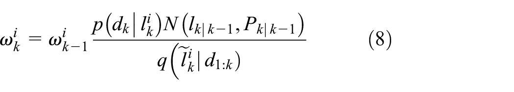
Substituting equation (5) into equation (8), we obtain $ω_{k}^{i} = p (d_{k} | l_{k}^{i})$ , and normalize the weights by equation (9).

{\tilde{ω}}_{k}^{(i)} = \frac{ω_{k}^{(i)}}{\sum_{i = 1}^{N} ω_{k}^{(i)}}

(9)

Step 4: Resampling. The effective particle capacity is estimated using equation (9). The results of Step 3 are compared with the given threshold $N_{th}$ , and if $N_{eff}$ < $N_{th}$ , the particle set is resampled. After resampling, the weights of all particles become $1 / N$ .

N_{eff} = \frac{1}{\sum_{i = 1}^{N} {({\tilde{ω}}^{(i)})}^{2}} < N_{th}

(10)

Step 5: State estimation. Get the estimate $\hat{l} = \sum_{i = 1}^{N} {\tilde{w}}_{k}^{(i)} {\tilde{l}}_{k}^{(i)}$ at moment k, return to step 1 and recursively calculate the state estimate for the next moment based on the observations input to the Bayesian network.

The optimization of Gaussian particle filtering algorithm based on firefly algorithm

Gaussian distribution is chosen as the important density function to make the particle distribution as close as possible to the system state probability density. This can improve the sampling efficiency and reduce particle degradation compared with the standard particle filtering algorithm. However, in the resampling step of the Gaussian particle filtering algorithm, particles with high weights are copied and particles with low weights are discarded, which may lead to the majority of particles being the descendants of a few particles, reducing the diversity of particles. In extreme cases, it may lead to the phenomenon of sample scarcity.^22,23 Given the problems existing in the Gaussian particle filtering algorithm, an effective method is to improve the resampling process and intelligent optimization algorithm.

The swarm intelligence optimization algorithm has received extensive attention due to its remarkable optimization effect, few adjustment parameters, and concise mathematical theory. Combining swarm intelligence optimization algorithms with practical problems is a hotspot of current research. In this paper, the firefly algorithm²⁴ of the swarm intelligence optimization algorithm is selected to optimize the Gaussian particle filtering algorithm. The specific optimization algorithm steps are as follows.

Step 1: Set the required parameters. Particle number N, maximum attractiveness β, step size factor α, media attractiveness factor γ, maximum iteration times m, and tracking threshold T are set.

Step 2: Particle initialization and importance sampling. The particle set ${l_{0}^{(i)}}_{i = 1}^{N}$ is obtained according to the prior distribution $p (l_{0})$ , the particle set is Gaussian filtered to obtain the new particle set ${l_{k}^{(i)}}_{i = 1}^{N}$ , and the Gaussian filter function is used as the importance density function. The Gaussian filter function is calculated as equation (5).

Step 3: The firefly algorithm guides the particles to move. Define the fitness function as.

Y = \exp [- {(z_{k} - {\hat{z}}_{k / k - 1}^{i})}^{2}]

(11)

Where $z_{k}$ is the latest measured value and ${\hat{z}}_{k / k - 1}^{i}$ is the predicted measured value. The firefly optimization algorithm determines the luminance by calculating the fitness function value, and the larger the fitness value, the higher its corresponding luminance. The luminance of each particle is determined by the latest measurement value in the optimization algorithm, and the position update equation guides the particles with low luminance to move to the particles with high luminance. The position update equation is shown in equation (12).

l_{i}^{t + 1} = ω l_{i}^{t} + β_{0} e^{- γ_{i}^{2}} (l_{j}^{t} - l_{i}^{t}) + α (R - 0.5)

(12)

where ω is the inertia weight factor, which is generally taken as a constant in the range of 0∼1, and R∈[0–1] is a random number.

Step 4: Calculate the weights of each particle after moving. The new particle set ${l_{1}^{(i)}}_{i = 1}^{N}$ is obtained after the movement of low luminance particles to high luminance particles in step 3, and the importance weights of each particle in the new particle set are calculated and normalized according to the Gaussian particle filtering algorithm. The calculation equation is shown in equations (8) and (9).

Step 5: Resampling. The resampling process needs to determine whether the updated particle weights satisfy equation (10). If it is satisfied, resampling is performed by Gaussian particle filtering; if not, no resampling is required.

Step 6: State output: Determine whether the maximum set number of iterations m and tracking threshold T are reached, if not, go to step 3, if it is reached, output the estimated value of the particle after moving.

The specific algorithm block diagram is as follows (Figure 6).

Figure 6.

Algorithm flow chart.

Experiments and case study

Firstly, suitable specimens are selected and fatigue experiments are conducted on a hydraulic servo fatigue tester to obtain real crack propagation data. In addition, the case study is performed based on the real crack propagation data, and Bayesian inference is performed using the Gaussian particle filtering algorithm and optimized Gaussian particle filtering algorithm, respectively, for comparative analysis.

Fatigue test

The steel plate material used in this paper is Q235. The specimens with the length L_a = 400 mm, the width W = 80 mm, and the thickness T = 8 mm are tested under the initial load peak 90 MPa,²⁵ the maximum reference load is 57.9 kN, and the stress ratio is 0.1. The specimen is shown in Figure 7, and the setting of the cyclic load spectrum is shown in Figure 8.

Figure 7.

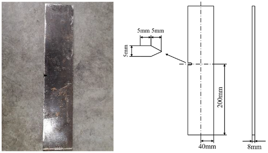
Fatigue crack propagation specimens.

Figure 8.

Fatigue test load spectrum.

Six specimens with the same dimensions and the position of pre-cracks were designed for the test. The experiment was conducted on the MTS 322 hydraulic servo fatigue tester. The lower hydraulic chuck was fixed and the upper hydraulic chuck was connected to the hydraulic rod to move with the hydraulic rod. The tensile cyclic load was output to the clamped metal plate with a load error of 1%. The hydraulic servo fatigue tester and the clamping process are shown in Figure 9.

Figure 9.

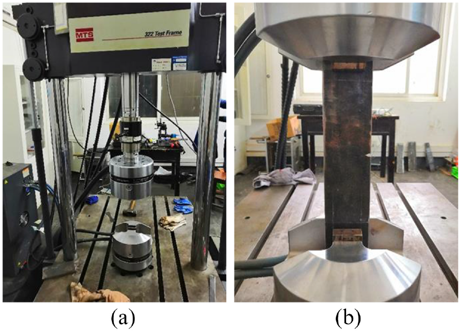
Experimental equipment and specimen clamping: (a) MTS 322 hydraulic servo fatigue tester and (b) experimental equipment after clamping.

The crack length is measured by the crack width gauge. This paper only considers the measurement length of the crack in one direction. The crack width gauge enlarges the crack section to complete the measurement of the crack propagation length. The maximum magnification is 40 times, and the accuracy is 0.02 mm. The crack measurement process is shown in Figure 10. The fatigue experiment consisted of two stages: the first stage was the pre-cracks stage, and the specimen was cyclically loaded to make the crack propagate to the design length of 28 mm. 10,000 cycles of load were used to measure the crack length during the pre-cracks stage using a crack gauge, and the crack length was measured every 1000 cycles after the crack propagation length was over 20 mm, and every 100 cycles of load were used to measure the crack propagation until it was close to 28 mm. The second stage was the experiment stage so that the crack propagated 1, 2, 3, and 4 mm based on the initial crack, the experimental process was measured once per 1000 cycles, and measured once per 100 cycles of load near the propagation of 1 mm. The progress of crack propagation is shown in Figure 11.

Figure 10.

Schematic diagram of crack width gauge and measurement effect: (a) crack width gauge and (b) schematic diagram of measurement effect.

Figure 11.

The process of Fatigue crack propagation: (a) prefabricated crack stage and (b) experimental stage.

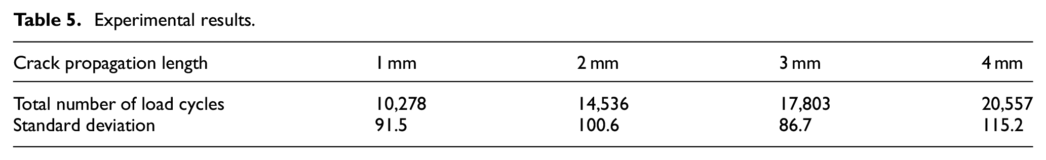
The total number of cycles applied to the load when the crack propagated to 1, 2, 3, and 4 mm were recorded respectively during the experiment. To reduce accidental error, the experimental data of the six specimens were averaged and the experimental results were shown in Table 5.

Table 5.

Experimental results.

Crack propagation length	1 mm	2 mm	3 mm	4 mm
Total number of load cycles	10,278	14,536	17,803	20,557
Standard deviation	91.5	100.6	86.7	115.2

In this paper, the 1–3 mm nodes in this experimental result are regarded as the input nodes of crack observations $L^{obs}$ , which are the diagnostic optimization nodes, and the 4 mm nodes are used as the nodes for testing the prediction effect.

Case study

The main objective of the fatigue crack propagation model based on the dynamic Bayesian network is to achieve a dynamic following of fatigue crack propagation and accurate knowledge of the current nodal crack state by updating the calibration uncertainty parameters through inference of the optimized Gaussian particle filtering algorithm. According to the previous experimental results, experimental instrument errors, and simulation experience, the prior distribution of parameters is defined as follows: cyclic load P = U (88.6704, 92.2896) MPa, simulation material parameters C₃ = U (1.935 × 10⁻⁷, 2.365 × 10⁻⁷), C₄ = U (4.815, 5.885). In this case, the initial crack length is assumed to be a deterministic value and each particle group generates 50 particles according to the initial probability distribution. The total number of load cycles of the experimental results is input as the observed value when the crack propagates to 1, 2, and 3 mm, respectively, and the effect of measurement noise is ignored. The nodes are updated using the Bayesian inference algorithm and the state is predicted for comparison when the crack propagates to 4 mm. The local particle coarsening method and the reduced model nonlinearity method are used to simplify the prediction model. 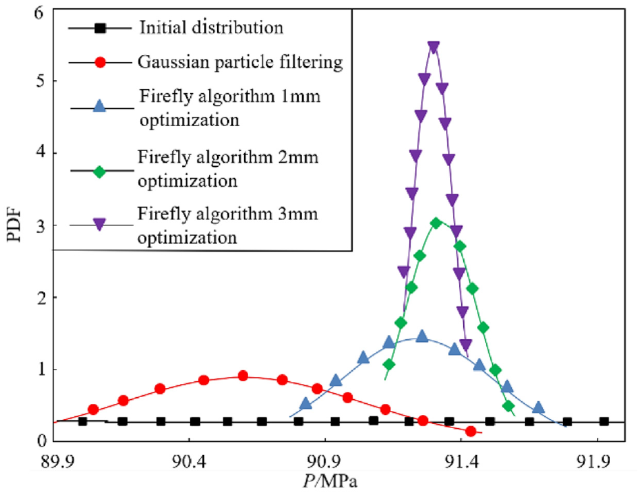The simplified reduced order model is used in the particle filtering prediction stage of $Δ L_{t}$ acquisition. The probability density functions of the three parameters are fitted according to the distribution states after obtaining the observed values as shown in Figures 12 to 14.

Figure 12.

The probability distribution of the load P after each optimization.

Figure 13.

The probability distribution of C₃ after each optimization.

Figure 14.

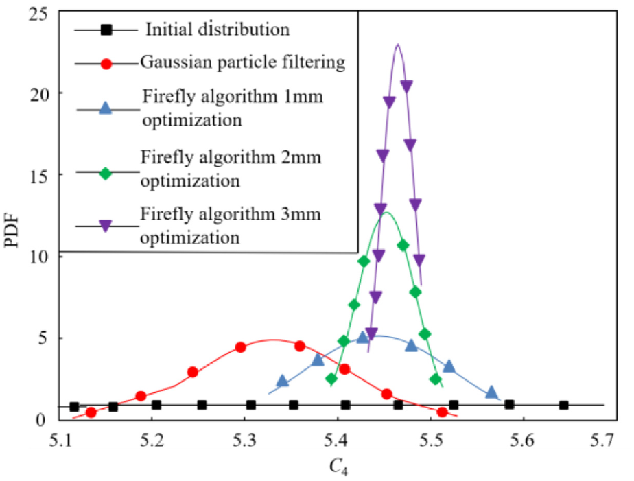
The probability distribution of C₄ after each optimization.

The results show that the uncertainty of the parameter variables decreases with each update, and the Gaussian particle filter and the Firefly algorithm 1 mm optimization have less influence on the particle uncertainty. Along with the optimization process, the particles quickly converge near the high-luminance particles, and the uncertainty is greatly reduced. It can be seen that, compared with the Gaussian particle filtering algorithm, the Gaussian particle filtering algorithm optimized by the firefly algorithm can accelerate the speed of particle convergence, making the particles converge quickly near the true value.

Figure 15 shows the comparison of crack propagation prediction with prior parameters obtained by Gaussian particle filter algorithm, crack propagation prediction by Gaussian particle filter algorithm optimized by firefly algorithm, and traditional crack propagation prediction without considering uncertainty factors. The results show that the errors in crack loading cycles accumulate at each correction point due to the uncertainty of the individual prior parameters. At 1 mm, the optimized Gaussian particle filtering algorithm corrects the load cycle offset 1130 times, reducing the error from 12.6% to 1.6%; at 2 mm, it corrects the offset 2239 times, reducing the error from 15.6% to 0.85%; at 3 mm, it corrects the offset 3110 times, reducing the error from 19.6% to 0.69%, and the error comparison is shown in Figure 16. The final 4 mm prediction result has an error of 2.8% compared with the real data. Compared with the traditional Gaussian particle filtering algorithm, the optimization method used in this paper reduces the error by 81.4%; compared with the traditional prediction method that does not consider uncertain factors, the optimization method used in this paper reduces the error by 74.3%. In summary, the proposed method can effectively improve the prediction accuracy of the fatigue crack propagation model while improving the computing efficiency.

Figure 15.

Comparison of crack propagation prediction results.

Figure 16.

Error comparison chart.

Conclusion

In this paper, a prediction method for fatigue crack propagation based on a dynamic Bayesian network is proposed. In this method, the dynamic Bayesian network and the simulation model are firstly constructed to represent the evolutionary process of crack propagation and the propagation of uncertainty factors. The optimized Gaussian particle filtering algorithm is used as the inference algorithm to update the system state and parameters in real-time. Finally, the proposed method is validated by experiments and case studies. The results show that:

The optimized Gaussian particle filtering algorithm is used as the inference algorithm, which can reduce the prediction error from 15.03% to 2.8%, compared with the traditional Gaussian particle filtering algorithm, and the accuracy of prediction accuracy can be improved by 81.4% while accelerating the operation speed.

The use of the simplification method of the finite element shortens the simulation time from 96 to 3.2 min, and the accuracy error is 1.28% of the full-order model, which effectively shortens the simulation time based on the low degree of accuracy impact.

Footnotes

Handling Editor: Chenhui Liang

Declaration of conflicting interests

The author(s) declared no potential conflicts of interest with respect to the research, authorship, and/or publication of this article.

Funding

The author(s) disclosed receipt of the following financial support for the research, authorship, and/or publication of this article: This work was partially supported by the Fundamental Research Funds for the Central Universities, project number 215218003. The authors have also received support from State Administration for Market Regulation Science and Technology Planned Project (Project No. 2021MK043).

ORCID iD

Zhiping Liu

References

Jiang

Hopman

Surface crack growth in offshore metallic pipes under cyclic loads: a literature review. J Mar Sci Eng 2020; 8: 339.

Paris

Erdogan

A critical analysis of crack propagation laws. J Basic Eng 1963; 85: 528–533.

Long

Tian-li

Hao

Stochastic modeling of metal fatigue crack growth using proportional Paris law and inverse gaussian process. Eng Mech 2021; 38: 238–247.

Martínez

Chakraborty

Tesfamariam

Machine learning assisted stochastic-xfem for stochastic crack propagation and reliability analysis. Theor Appl Fract Mech 2021; 112: 102882.

Bartram

Mahadevan

Integration of heterogeneous information in SHM models. Struct Control Health Monit 2014; 21: 403–422.

Yang

, et al. Digital twin for the structural health management of reusable spacecraft: a case study. Eng Fract Mech 2020; 234: 107076.

Mahadevan

Ling

, et al. Dynamic Bayesian network for aircraft wing health monitoring digital twin. AIAA J 2017; 55: 930–941.

Song

Tang

, et al. A digital twin approach based on nonparametric Bayesian network for complex system health monitoring. J Manuf Syst 2021; 58: 293–304.

Fang

Wang

, et al. Fatigue Crack growth prediction method for offshore platform based on digital twin. Ocean Eng 2022; 244: 110320.

10.

Yang

Peng

, et al. Remaining useful life prognostic of power metal oxide semiconductor field effect transistor based on improved particle filter algorithm. Adv Mech Eng 2017; 9: 1687814017749324.

11.

Wang

Huang

An improved particle filtering algorithm for aircraft engine gas-path fault diagnosis. Adv Mech Eng 2016; 8: 1687814016659602.

12.

Chen

Yuan

Qiu

, et al. On-line prognosis of fatigue crack propagation based on gaussian weight-mixture proposal particle filter. Ultrasonics 2018; 82: 134–144.

13.

Yang

Gao

Lamb wave-minimum sampling variance particle filter-based fatigue crack prognosis. Sensors 2019; 19: 1070.

14.

Jia

Zhang

, et al. Failure analysis of composite laminates under transverse shear load via XFEM. Compos Struct 2021; 262: 113615.

15.

Liu

Detail feature recognition and decomposition in solid model. Comput Aided Des 2002; 34: 405–414.

16.

Kwon

Chul Kim

Mun

, et al. Graph-based simplification of feature-based three-dimensional computer-aided design models for preserving connectivity. J Comput Inf Sci Eng 2015; 15: 031010.

17.

Wang

H-H

Fang

Liu

D-J

, et al. Fatigue crack growth prediction method under variable amplitude load based on dynamic Bayesian network. Eng Sci 2021; 55: 280–288.

18.

Dong

Testing for Paris coefficients C, m and ΔK_(th) of Q235. J Mech Strength 2003; 2: 215–218.

19.

Liu

, et al. Fatigue crack propagation path and life prediction based on XFEM. J Northwestern Polytech Univ 2019; 37: 737–743.

20.

Deng

Xiong

, et al. Analysis of biaxial non-proportional low-cycle fatigue crack propagation behavior of hull plate with an inclined crack based on accumulative plasticity. J Fail Anal Prev 2021; 21: 1345–1361.

21.

Kotecha

Djuric

PM.

Gaussian sum particle filtering. IEEE Trans Signal Process 2003; 51: 2602–2612.

22.

Dynamic resampling particle filter adaptive to changes in system model. J Contr Theor Appl 2011; 9: 584–588.

23.

Sattar

Sun

Deterministic resampling: unbiased sampling to avoid sample impoverishment in particle filters. Signal Process 2012; 92: 1637–1645.

24.

Yang

X-S

Firefly algorithm: recent advances and applications. Int J Swarm Intell 2013; 1: 36–50.

25.

Fan

High cycle fatigue behavior evaluation of Q235 steel based on energy dissipation. J Mech Eng 2018; 54: 1.

Prediction of fatigue crack propagation based on dynamic Bayesian network

Abstract

Keywords

Introduction

The simplification methods of the finite element model

The dynamic Bayesian network for crack propagation

Analysis of uncertain factors

Construction of the dynamic Bayesian network

Bayesian inference based on optimized Gaussian particle filtering algorithm

Equation of state for fatigue crack propagation

Gaussian particle filtering algorithm

The optimization of Gaussian particle filtering algorithm based on firefly algorithm

Experiments and case study

Fatigue test

Case study

Conclusion

Footnotes

Declaration of conflicting interests

Funding

ORCID iD

References