Rolling bearing fault diagnosis based on improved VMD-adaptive wavelet threshold joint noise reduction

Abstract

Due to the fault vibration signal of the rolling bearing is greatly interfered by the background noise, the fault features are easily submerged and result in a low fault diagnosis accuracy. A novel fault diagnosis method of rolling bearing is proposed based on improved VMD-adaptive wavelet threshold combined with noise reduction in this paper. Firstly, the modal components are obtained based on VMD decomposition; Secondly, the dual determination criteria of sample entropy and correlation coefficient are constructed to filter the components; Subsequently, an adaptive wavelet thresholding function is proposed, and quadratic noise reduction is applied to mixed IMFs, which in turn reconstructs each component to achieve joint noise reduction. Finally, based on traditional machine learning and deep learning diagnosis methods, the features of noise reduction signals are extracted to realize fault diagnosis. By verifying and analyzing the simulated signal with the measured signal, noise components, the expression of fault characteristics, and the accuracy of fault diagnosis are eliminated, enhanced, and improved.

Introduction

Rolling bearings are key components supporting the operation of rotating machinery and equipment, and relevant data show that about 30% of rotating machinery failures are caused by rolling bearings, ¹ and their operating conditions directly affect the performance and safety of machinery and equipment. Therefore, the effective diagnosis of rolling bearing failure is of great significance to improve the service life and working performance of mechanical equipment. ² In the case of early failure of rolling bearings, the vibration signal contains a large amount of noise information due to the influence of the location layout of the sensor and the surrounding environment. It makes failure characteristic signal not obvious and difficult to be detected. ³ Therefore, an effective early fault signal noise reduction method is essential for bearing fault diagnosis.

In view of the non-stationary, nonlinear and coupled modulation characteristics of rolling bearing fault vibration signals, ⁴ scholars have applied signal decomposition methods to the field of noise reduction research, such as empirical mode decomposition (EMD), ⁵ ensemble empirical mode decomposition (EEMD), ⁶ complete ensemble empirical mode decomposition (CEEMD), ⁷ and so on. Compared with the above methods, variational mode decomposition (VMD) ⁸ can effectively avoid the problems of modal mixing and endpoint effects, and at the same time can suppress the interference of noise. Wavelet threshold noise reduction ⁹ is a time-scale analysis method with the advantages of multi-resolution analysis and simple noise reduction principle. It is usually combined with the VMD decomposition algorithm to perform a secondary noise reduction process on the intrinsic mode function (IMFs), which in turn reconstructs the components to achieve joint noise reduction. Liu et al. ¹⁰ combined VMD decomposition and improved wavelet thresholding for noise reduction of vibration information of planetary wheel wear faults and crack faults. Chen et al. ¹¹ proposed a rolling bearing fault feature extraction method with optimized VMD and improved threshold noise reduction, and it was verified that the fault features were more obvious after the noise reduction by this method. Chen et al ¹² proposed a method based on VMD and alignment entropy combined with wavelet noise reduction, which was applied to the noise reduction processing of wind turbine vibration signals in strong noise background. Liu et al. ¹³ proposed a noise reduction method of VMD combined with soft threshold wavelet for rolling bearing fault vibration information.

The results show that the VMD combined with wavelet threshold noise reduction can effectively remove the noise components from the signal and extract the weak features of the rolling bearing vibration signal at the early stage of degradation in the strong noise background. However, the noise information is distributed among the components after VMD decomposition, and the IMF components need to be selected and given the optimal subsequent noise reduction process. Therefore, the selection of IMF components and the optimization of wavelet threshold function are worthy of further study.

Regarding the selection of IMF components, Cui et al. ¹⁴ used the Kurtosis criterion to identify IMFs with prominent fault information to reconstruct the signal. Li et al. ¹⁵ selected IMFs with rich fault information based on frequency band entropy. Jin et al. ¹⁶ selected the best IMF component based on the Pearson correlation. Yan et al ¹⁷ used fault feature ratio to select IMFs rich in fault information as the main component for the next step of spectrum analysis. Cao et al. ¹⁸ measured the noise content of each IMF component based on permutation entropy and classified each IMF component according to the noise content. Akhenia et al. ¹⁹ selected the IMF components with maximum energy and minimum Shannon entropy as valid components to generate spectrograms based on the ratio of maximum energy to Shannon entropy criterion. Kumar et al. ²⁰ measured the similarity between each IMF and the original signal based on the dynamic time warping criterion to select the valid components. Liang et al. ²¹ screened two IMF components with maximum fault information for reconstruction based on the improved kurtosis criterion combined with the Holder coefficient criterion. Chen et al. ²² used sample entropy to classify the components into noise IMF components, mixed IMF components, and useful IMF components. The selection of IMF in the above studies is often based on a single indicator or only distinguishes between valid and invalid components (dichotomous classification), which may lead to a less accurate type discrimination of components. The problem that valid information is eliminated and irrelevant information is retained exists.

Regarding the optimization of the wavelet thresholding function, Xie et al. ²³ considered the effect of the number of layers of wavelet decomposition and improved the thresholding function to reduce the bias due to inaccurate thresholding. Chen and Zhang ²⁴ improved the wavelet thresholding function and combined it with median filtering to set different thresholds for each level of wavelet details. Li et al. ²⁵ proposed a continuously derivable threshold function at the threshold, where the coefficients below the threshold are adjusted by a power function instead of being set to zero to prevent the loss of useful information. Chegini et al. ²⁶ proposed an improved threshold function, which makes the function adjust between soft and hard functions by artificially setting the size of the parameters. Li et al. ²⁷ used the attenuation property of the exponential function to retain a part of wavelet coefficients close to the wavelet threshold to prevent the problem of excessive noise reduction. Dalei et al. ²⁸ improved the wavelet semi-soft threshold function and determined the value of the adjustment parameter a in it. The adjustment parameters of the optimized wavelet threshold function in the above study cannot be set adaptively according to the noise content of the signal, and the robustness is poor too.

In this paper, for the noise reduction problem of rolling bearing vibration signal, the IMF component selection and wavelet threshold function optimization are studied, and a joint noise reduction method based on improved VMD-adaptive wavelet thresholding is proposed. Firstly, the IMF components after VMD decomposition are selected based on the dual determination criteria of sample entropy and correlation coefficient; Secondly, an adaptive wavelet threshold function is proposed to adaptively adjust the noise reduction form according to the noise content degree of the noise-containing components, to perform secondary noise reduction for mixed IMFs, and to reconstruct each component to realize joint noise reduction. Finally, the traditional machine learning and deep learning diagnosis methods are adopted respectively to realize the bearing fault diagnosis. At the same time, the improvement of the diagnosis accuracy by the noise reduction method in this paper is verified. The analysis results of simulated and measured signals show that the joint noise reduction method proposed in this paper has better noise reduction effect and self-adaptability, which effectively enhances the expression ability of features and improves the accuracy of diagnosis.

Improved VMD-adaptive wavelet threshold joint noise reduction

VMD

VMD is a non-recursive, adaptive signal decomposition algorithm that decomposes the original signal into a series of intrinsic mode function sums with finite bandwidth and center frequency, and each IMFs is defined as an FM-AM signal. The formula is as follows:

$$u_k\left(t\right)=A_k\left(t\right)\cos \left({\Phi }_k\left(t\right)\right)$$

(1)

Where: $A_k\left(t\right)$ is the instantaneous amplitude and ${\Phi }_k\left(t\right)$ is the instantaneous phase.

Constrained variational models are constructed by estimating the bandwidth of each IMFs using the demodulation method. The formula is as follows:

$$\begin{array}{c}\underset{\left\{u_k\right\},\left\{{\omega }_k\right\}}{min}\left\{\sum _k{\Vert {\partial }_t[(\mathrm{\delta }\left(t\right)+\frac{j}{\pi t})*u_k\left(t\right)]e^{-j{\omega }_{k}t}\Vert }_2^2\right\}\hfill \\ s.t.\sum _k{u}_k=f(t)\hfill \end{array}$$

(2)

Where: $\left\{u_k\right\}=\{u_1,...,u_K\}$ is the decomposed K IMFs, and $\left\{{\omega }_k\right\}=\{{\omega }_1,...,{\omega }_K\}$ is the corresponding center frequency of each component.

To solve the above model, the Lagrangian operator $\lambda$ and the quadratic penalty factor $\alpha$ are introduced, and the constrained variational problem is transformed into an unconstrained variational problem with an augmented Lagrangian function expression as:

$$\begin{array}{c}L(\left\{u_k\right\},\left\{{\omega }_k\right\},\mathrm{\lambda })=\alpha \sum _k{\Vert {\partial }_t[(\mathrm{\delta }\left(t\right)+\frac{j}{\pi t})*u_k\left(t\right)]e^{-j{\omega }_{k}t}\Vert }_2^2\hfill \\ +\Vert f\left(t\right)-\sum _k{u}_k\left(t\right)\Vert \begin{array}{c}2\hfill \\ \multicolumn{1}{c}{2}\end{array}+〈\mathrm{\lambda }\left(t\right),f\left(t\right)-\sum _k{u}_k\left(t\right)〉\hfill \end{array}$$

(3)

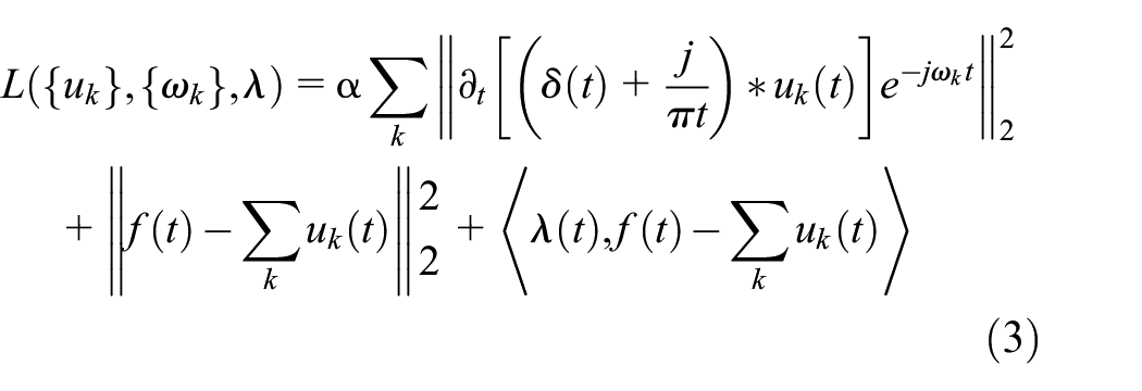
The optimal solution of the variational constraint model is obtained by alternately updating $u_k^{n+1}$ , ${\omega }_k^{n+1}$ , and ${\mathrm{\lambda }}^{n+1}$ using the alternating direction method of the multiplicative operator. The update equation is as follows.

$$\begin{array}{c}\multicolumn{1}{c}{{\hat{u}}_k^{n+1}\left(\omega \right)=\frac{\hat{f}\left(\omega \right)-\sum _{i\ne k}{\hat{u}}_i\left(\omega \right)+\frac{\hat{\lambda }\left(\omega \right)}{2}}{1+2a{(\omega -{\omega }_k)}^2}}\\ \multicolumn{1}{c}{{\omega }_k^{n+1}=\frac{{\int }_0^{\infty }\omega {\left|{\hat{u}}_k\left(\omega \right)\right|}^{2}d\omega }{{\int }_0^{\infty }{\left|{\hat{u}}_k\left(\omega \right)\right|}^{2}d\omega }}\\ {\hat{\lambda }}^{n+1}\left(\omega \right)={\hat{\lambda }}^n\left(\omega \right)+\tau [\hat{f}\left(\omega \right)-\sum _k{\hat{u}}_k^{n+1}\left(\omega \right)]\hfill \end{array}$$

(4)

The termination constraint is given by: (in equation, $\mathrm{\epsilon }$ notes convergence accuracy)

$$\sum _k\Vert {\hat{u}}_k^{n+1}-{\hat{u}}_k^n{\Vert }_2^2/\Vert {\hat{u}}_k^n{\Vert }_2^2<\mathrm{\epsilon }$$

(5)

The noise content of each IMFs obtained by decomposition is basically different, and the sample entropy and correlation coefficient are introduced as the quantification criteria of the noise content of each IMFs in order to give the optimal treatment.

Improved VMD based on the dual determination criterion of sample entropy-correlation coefficient

The calculation of sample entropy (SE) does not depend on the length of the data and is not affected by the intrinsic characteristics of the signal, the sample entropy has a high accuracy. The complexity and disorder of a signal increases when it is disturbed by noise, and the sample entropy value is larger. ²⁹ Let a one-dimensional time series of length N be $X=\{x_1,x_2,x_3,...,x_N\}$ . Its sample entropy is defined as follows:

$$S_E(m,r,N)=-\ln \left[\frac{A^m\left(r\right)}{B^m\left(r\right)}\right]$$

(6)

Where: m is the number of embedding dimensions; r is the similarity tolerance value; $A^m\left(r\right)$ is the sum of the number of time series with spacing less than r in m + 1 dimensions; $B^m\left(r\right)$ is the sum of the number of time series with spacing less than r in m dimensions; the embedding dimension m is 2; and the similarity tolerance value r is one-fifth of the standard deviation of the time series X.

Calculate the sample entropy $S_X$ of the original signal and the sample entropy $S_i$ of each IMFs. The screening criteria are as follows: The components of $S_i>1.1S_X$ are noisy IMFs, and this type of component has a very large noise content and almost no useful components; The components of $S_i\le 0.3S_X$ are useful IMFs, and this type of component is basically composed of useful signals; The component of $0.3S_X<S_i\le 1.1S_X$ are residual IMFs, and this type of component is composed of some noise components and useful components. ²²

Due to the poor correlation between the noise information or the noise component caused by endpoint oscillations and the original signal, noisy IMFs can be determined by the correlation coefficient (Corr), which is expressed as: Where: X and Y are one-dimensional time series of length N.

$$P=\frac{{\sum }_{i=1}^N(X_i-\overline{X})(Y_i-\overline{Y})}{\sqrt{{{\sum }_{i=1}^N(X_i-\overline{X})}^2*{{\sum }_{i=1}^N(Y_i-\overline{Y})}^2}}$$

(7)

The correlation coefficients of each residual component with the original signal are further calculated, defining: The components of $P_i\le 1$ are noisy IMFs; The components of $P_i>1$ are mixed IMFs, ³⁰ subject to further noise reduction.

Due to the richness of rolling bearing vibration signals, the screening of IMFs by a single indicator may result in valid components being rejected and irrelevant components being retained. ³¹ Therefore, this paper constructs a dual determination criterion of sample entropy and correlation coefficient, firstly, using sample entropy to analyze the noise content of each component and filter it, and further using correlation coefficient to measure the correlation degree between the residual IMFs and the original signal to ensure the accurate classification of mixed IMFs and noisy IMFs. Stable screening of the maximum correlation components of the periodic fault pulse and the original signal in the measured signal, effectively reducing noise interference.

Adaptive wavelet threshold function noise reduction

A wavelet thresholding function is applied to mixed IMFs for secondary noise reduction. However, the conventional hard threshold function is discontinuous and has intermittent points in the wavelet domain, making the reconstructed signal oscillatory. Although the soft threshold function is continuous, there is a constant error between the reconstructed signal and the real signal. Moreover, the noise reduction forms of the above two threshold functions are single fixed and lack of robustness. Therefore, on the basis of traditional wavelet threshold, this paper proposes an adaptive continuous wavelet threshold function based on sample entropy. The expression is as follows:

$$d^{*}=\{\begin{array}{c}\mathrm{sgn}\left(d\right)(\left|d\right|-\mathrm{bT})\begin{array}{c}\left|d\right|>T\hfill \end{array}\hfill \\ \multicolumn{1}{c}{\mathrm{sgn}\left(d\right)\frac{e^{10*b(\frac{\left|d\right|}{T}-1)}}{1-a}(\left|d\right|-\mathrm{aT})(1-b)\begin{array}{c}\mathrm{aT}\le \left|d\right|\le T\hfill \end{array}}\\ \multicolumn{1}{c}{0\begin{array}{c}\left|d\right|<\mathrm{aT}\hfill \end{array}}\end{array}$$

(8)

In the formula: $d$ is the wavelet coefficient; $d^{*}$ is the wavelet coefficient after noise reduction; T is the threshold; a is an adjustable parameter (0 < a < 1), so that the wavelet coefficient between the two thresholds can be denoised by using the exponential decay characteristic to avoid The problem of excessive noise reduction caused by direct zero setting, a value of 1/1.16 ²⁸ ; b is an adaptive parameter (0 ≤ b ≤ 1), which measures the noise level of the mixed IMFs, so that the threshold function can automatically adjust the noise reduction form according to the noise condition. The expression is as follows :

$$\{\begin{array}{c}b=\frac{{S_i}^{*}-0.3S_X}{0.3S_X}\begin{array}{c}0.3S_X<{S_i}^{*}<0.6S_X\hfill \end{array}\hfill \\ \multicolumn{1}{c}{b=1\begin{array}{c}{S_i}^{*}\ge 0.6\hfill \end{array}{S}_X}\end{array}$$

(9)

In the formula: S_X is the sample entropy of the original signal, 0.3S_X is the threshold value to distinguish useful IMFs from residual IMFs ²² ; ${S_i}^{*}$ is the sample entropy of mixed IMFs. When b tends to 0, a harder threshold function is used for noise reduction; otherwise, b tends to 1, a softer threshold function is used for noise reduction.

When the a value is fixed at 0.8, and the b value is 0.8, 0.5, and 0.2, the function image is shown in Figure 1.

Figure 1.

Adaptive wavelet threshold function image.

Firstly, the bias of the adaptive wavelet threshold function is tested.

$$\begin{array}{c}\underset{d\to +\infty }{lim}(d^{*}-d)=\underset{d\to +\infty }{lim}[\mathrm{sgn}\left(d\right)(d-\mathrm{bT})-d]=-\mathrm{bT}\hfill \\ \underset{d\to -\infty }{lim}(d^{*}-d)=\underset{d\to -\infty }{lim}[\mathrm{sgn}\left(d\right)(-d-\mathrm{bT})-d]=+\mathrm{bT}\hfill \end{array}$$

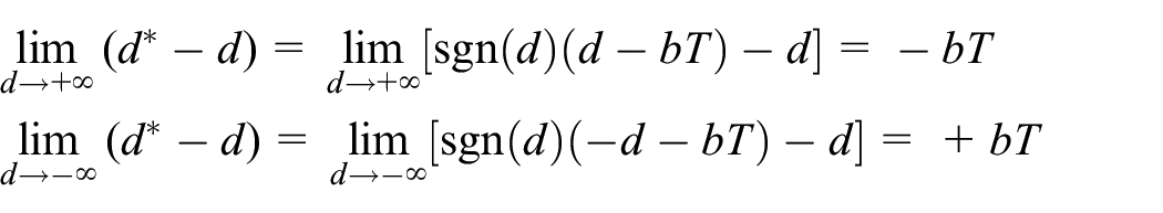
Second, the continuity of the adaptive wavelet threshold function is tested, when $d\to T^{+}$ , $d\to T^{-}$ ; when $d\to a{T}^{+}$ , $d\to a{T}^{-}$ .

$$\begin{array}{c}d*=\mathrm{sgn}\left(T^{+}\right)(T^{+}-b*T)=(1-b)*T\hfill \\ d*=\mathrm{sgn}\left(T^{-}\right)*\frac{e^{10b(\frac{T^{-}}{T}-1)}}{1-a}*(T^{-}-\mathrm{aT})*(1-b)=(1-b)*T\hfill \end{array}$$

$$\begin{array}{c}d*=\mathrm{sgn}\left(a{T}^{+}\right)*\frac{e^{10b(\frac{a{T}^{+}}{T}-1)}}{1-a}*(a{T}^{+}-\mathrm{aT})*(1-b)=0\hfill \\ d*=0\hfill \end{array}$$

In summary, the function is continuous at d = T and d = aT; at the same time, due to the adaptive adjustment of parameter b, the deviation is also adjusted accordingly. Therefore, the adaptive wavelet threshold function in this paper not only avoids the discontinuity of the hard threshold function, but also reduces the constant error of the soft threshold function. It can be adaptively adjusted according to the noise of the signal, which makes the application more flexible.

Improved VMD-adaptive wavelet threshold joint noise reduction

Based on the above algorithms and theories, this paper proposes an improved VMD-adaptive wavelet threshold function joint denoising method. The implementation steps are shown in Figure 2.

1. Perform VMD decomposition on the signal, and screen IMFs based on the dual determination criterion of sample entropy correlation coefficient.

2. Discard noisy IMFs, retain useful IMFs, and perform secondary noise reduction using adaptive wavelet thresholding functions for mixed IMFs.

3. Reconstruct IMFs to get denoised signal.

Figure 2.

The joint noise reduction flow chart of this paper.

Simulation signal test and analysis

In the vibration signal acquisition process, the real signal is disturbed by a large number of high-frequency noise signals and weak fault features are usually distributed in the low frequency band within 1 kHz due to the influence of mechanical equipment and the surrounding environment. ³ To verify the effectiveness of the noise reduction pre-processing algorithm proposed in this paper, a set of non-smooth, non-linear periodic amplitude-modulated frequency modulated signals are constructed to simulate the periodic signals of the faults; and Gaussian white noise and colored noise are added to simulate the interference noise signals in the high frequency band.

$$\begin{array}{l}{x}_1\left(t\right)=\sin \left(10\pi t+\frac{\pi }{5}\right)+\cos \left(80\pi t+\sin \left(10\pi t\right)\right)\\ x_2\left(t\right)=\left(1+0.3\cos \left(10\pi t\right)\right)\ast \sin \left(200\pi t\right)\\ f\left(t\right)=x_1\left(t\right)+x_2\left(t\right)+\mu \left(t\right)\end{array}$$

(10)

Where: t = [0, 1], the sampling frequency is 1000 Hz. $\mu \left(t\right)$ is the noise signal. The time and frequency domain waveforms before and after the addition of Gaussian white noise with SNR = 1 and colored noise with SNR = −2.0 are shown in Figure 3. The useful frequency components of the signal are 5, 40, and 100 Hz. The Gaussian white noise is uniformly distributed in the whole frequency domain, while the colored noise is mainly distributed in the high frequency band and has a higher amplitude compared with the white noise, and the two noise signals show different characteristics in the frequency domain.

Figure 3.

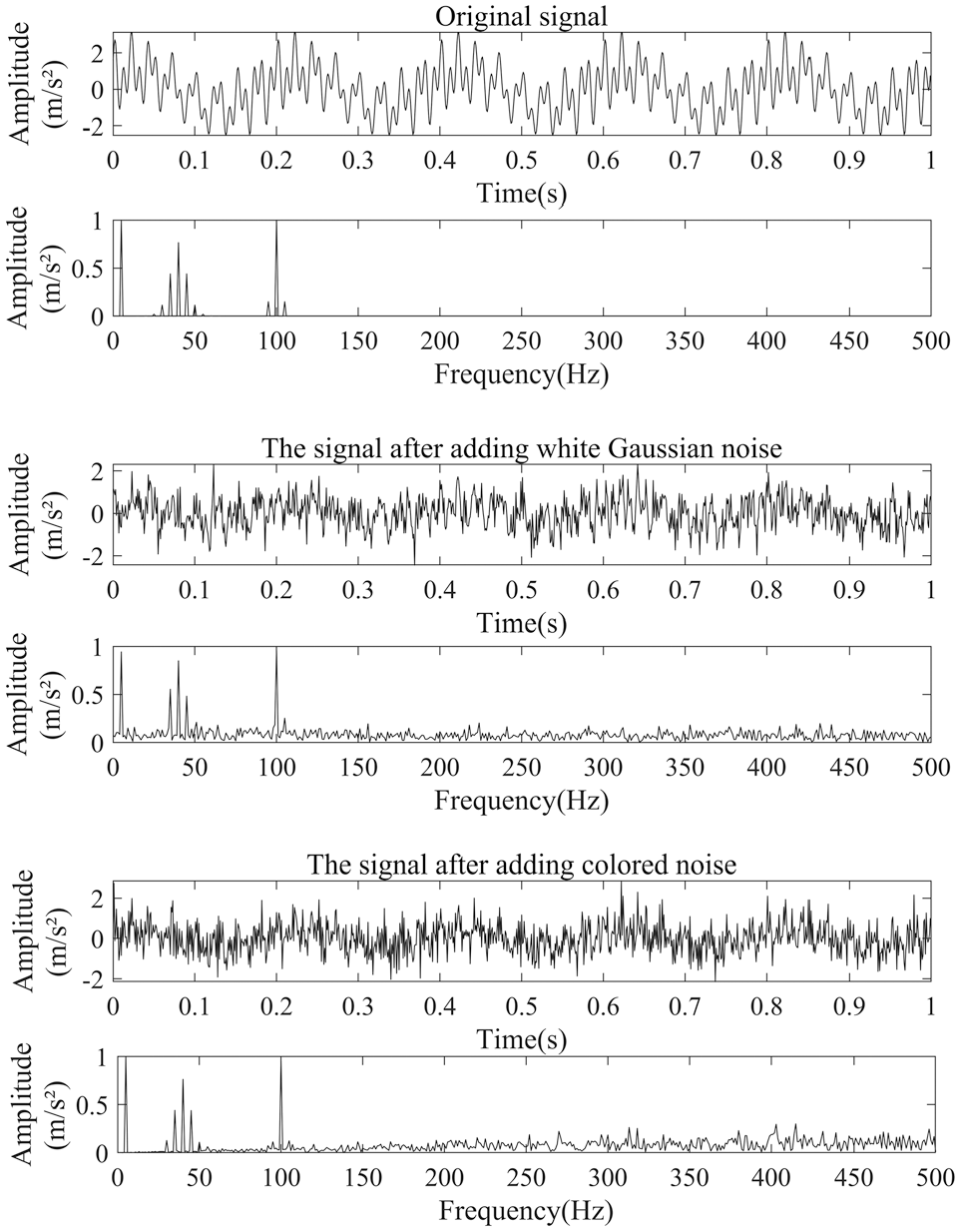
Waveform in time domain and frequency domain before and after adding noise.

VMD and IMFs selection

To verify the screening effect of the dual determination criterion on IMF components in this paper, the components were screened by the sample entropy criterion, ²² the ratio of maximum energy to Shannon entropy criterion (Ratio criterion), ¹⁹ the dynamic time warping criterion (DTW criterion), ²⁰ and the criterion in this paper. As an example, the parameters of VMD were determined by genetic algorithm for a signal containing white noise with SNR = 15, ¹³ and the calculation results and screening results based on each criterion are shown in Table 1.

Table 1.

Component screening fact sheet.

	IMF1	IMF2	IMF3	IMF4
SE	0.817	0.319	0.300	0.277
Corr	0.091	0.581	0.582	0.569
Ratio	30.57	160.48	163.57	156.09
Ratio normalization	0	0.981	1	0.968
DTW	812.3	577.4	567.6	819.7
DTW normalization	0.970	0.039	0	1
Se Criterion	Mixed IMFs	Useful IMFs	Useful IMFs	Useful IMFs
ratio Criterion	Mixed IMFs	Useful IMFs	Useful IMFs	Useful IMFs
DTW criterion	Mixed IMFs	Useful IMFs	Useful IMFs	Mixed IMFs
Dual determination criterion	Noisy IMFs	Useful IMFs	Useful IMFs	Useful IMFs

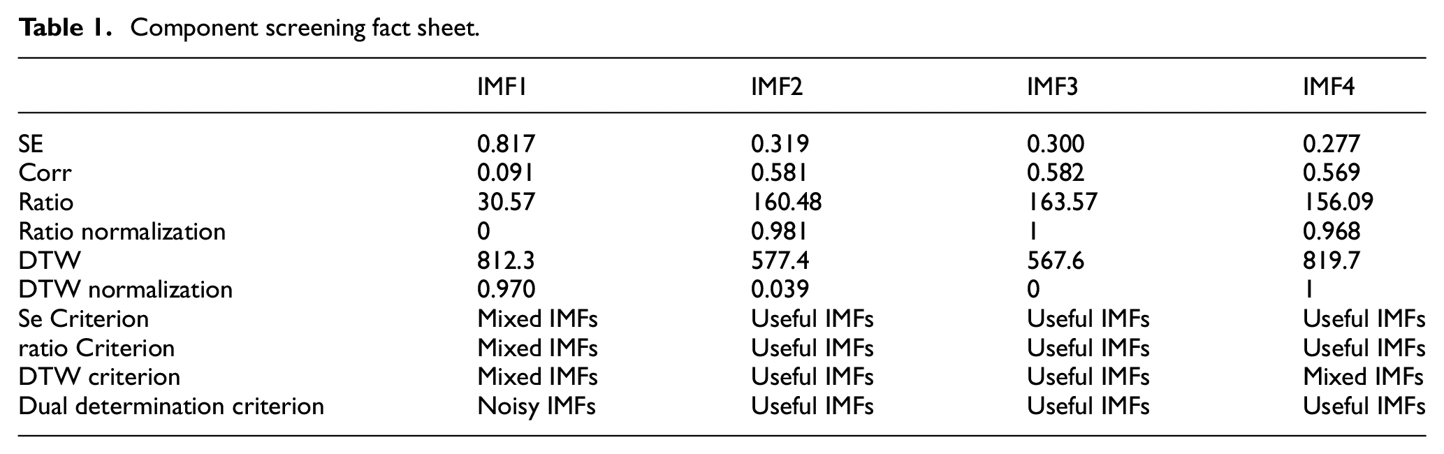
Among them, the ratio values and DTW values are normalized in order to specifically quantify the importance of IMFs when selecting IMF components based on the ratio criterion and DTW criterion. The rules of the ratio criterion are as follows: the components whose normalized ratio value is greater than 0.9 and less than or equal to 1 are regarded as useful IMFs conversely, they are regarded as mixed IMFs and require secondary noise reduction. The DTW criterion rule is as follows: the components whose normalized DTW values are greater than or equal to 0 and less than 0.1 are regarded as useful IMFs; conversely, they are regarded as mixed IMFs.

From Table 1, IMF2 and IMF3 were determined as useful IMFs by the above four criteria; IMF4 was determined as mixed IMFs by the DTW criterion and useful IMFs by the other three criteria. IMF1 was determined as noisy IMFs by the criteria of this paper and mixed IMFs by the other three criteria.

To check the merits of the screening results of each criterion, the spectral analysis of each component is shown in Figure 4. IMF4, IMF3, and IMF2 contain 5, 40, and 100 Hz frequency components and the amplitude of the frequency components at high frequencies are 0, which belong to useful IMFs; while IMF1 does not contain useful frequency components, which belong to noisy IMFs. The above analysis results are consistent with the results filtered by the criterion in this paper.

Figure 4.

Spectrum diagram of IMF.

In order to visualize the screening effect of each criterion, after the screening by each criterion, a hard threshold function is used for the secondary noise reduction and reconstruction. The signal-to-noise ratio and correlation coefficient were used as the evaluation indexes, and the noise reduction effect is shown in Table 2. The signal-to-noise ratio was 19.44 and the correlation coefficient was 0.994 after being screened by the double-judgment criterion and the secondary noise reduction, which was the best.

Table 2.

The noise reduction result.

	Criteria for IMFs selection	SNR	Corr
SNR = 15, white noise	SE criterion	19.05	0.993
	Ratio criterion	19.05	0.993
	DTW criterion	18.65	0.980
	Dual determination criterion	19.44	0.994

In summary, the ratio criterion and the DTW criterion, both based on a single indicator, only distinguish between useful IMFs and mixed IMFs, which leads to the exclusion of effective components and the retention of irrelevant components, thus affecting the effect of secondary noise reduction. The sample entropy criterion distinguishes between useful IMFs, mixed IMFs, and noisy IMFs, but based on a single indicator, it is easy to discriminate some component types inaccurately. The criterion in this paper combines the dual screening of sample entropy and correlation coefficient, which quantifies the noise content of each IMF and measures the correlation between each IMF and the original signal, ensuring that the three component types are accurately classified and have better screening effects.

Joint noise reduction

To verify the robustness and noise reduction effect of the adaptive wavelet thresholding function in this paper, on the basis of the dual determination criterion in this paper, VMD + soft thresholding (VMD + soft), VMD + hard thresholding (VMD + hard), VMD + semi-soft thresholding (VMD + semi-soft), and the method in this paper are used for noise reduction of the signal containing white noise with SNR = 1 and the signal containing color noise with SNR = −2.0.

Considering the large number of IMFs, the process of determining the optimal wavelet decomposition parameters for each component individually is tedious and there is no quantitative indicator to measure the advantages and disadvantages of each parameter. Therefore, the best parameters are determined by wavelet decomposition of the original signal as the optimal parameters for wavelet decomposition of each IMF component.

Taking the simulated signal containing white noise with SNR = 1 as an example, the rules for selecting the wavelet decomposition parameters are as follows:

• ① Number of decomposition layers j: wavelet decomposition of the original signal, the ratio of the wavelet entropy of the second layer to the entropy of the original signal is 0.052, which is close to 5%, ³² and the optimal number of decomposition layers j = 2.

•   Wavelet basis and threshold determination principle: determined by exhaustive method respectively.

• ② Determination of wavelet basis: the number of decomposition layers j is taken as 2, and the threshold principle is tentatively set as sqtwolog threshold. Considering the wavelet bases of dbN, coifN, symN series are well matched with mechanical fault vibration signals and have the advantages of highlighting fault characteristics and so on. ¹³ The wavelet bases of the above series are selected respectively, and the original signal is processed by noise reduction using soft threshold, and the optimal base wavelet is selected according to the signal-to-noise ratio of the signal after noise reduction, and the results are shown in Table 3. Compared with the three, the wavelet base of coifN series has a good noise reduction effect, and the wavelet base is selected as: the wavelet base coif5 with the highest evaluation index.

• ③ Determination of the thresholding principle: take the number of decomposition layers j as 2, wavelet base as coif5, and select sqtwolog threshold, heursure threshold, minimaxi threshold, and rigrsure threshold for noise reduction of the original signal, and similarly select the optimal base wavelet according to the signal-to-noise ratio, and the results are shown in Table 4. The noise reduction effect of each threshold principle is approximately the same, considering minimaxi threshold and rigrsure threshold, most of the coefficients smaller than the threshold are set to zero, which can avoid the problem of excessive noise reduction caused by setting all of them to zero, ³³ and minimaxi threshold is finally chosen.

Table 3.

Wavelet bases of each series – noise reduction effect.

Wavelet basis	SNR	Wavelet basis	SNR	Wavelet basis	SNR
db2	4.76	sym2	4.76	coif2	5.30
db3	5.01	sym3	5.01	coif3	5.56
db4	5.27	sym4	5.29	coif4	5.72
db5	5.34	sym5	5.37	coif5	5.85
db6	5.45	sym6	5.47
db7	5.59	sym7	5.56

Table 4.

Principle of each threshold – noise reduction effect.

The principle of threshold	SNR	The principle of threshold	SNR
sqtwolog	5.85	minimaxi	5.86
heursure	5.85	rigrsure	5.85

After determining the parameters of wavelet decomposition, the above joint method is used to noise reduction of the signal containing white noise with SNR = 1. The time domain and frequency domain waveforms after noise reduction are shown in Figure 5, it can be seen that noise frequency components exist around 200 Hz for VMD + soft, VMD + hard, and VMD+semi-soft while noise components with high amplitude remain at 150 Hz after noise reduction by VMD + hard and VMD + semi-soft. The frequency components at 5, 40, and 100 Hz are prominent after noise reduction by the method in this paper, and the frequency amplitude above 200 Hz is zero, and the ability of the signal to express features is enhanced.

Figure 5.

Waveform in time domain and frequency domain after noise reduction.

The signal-to-noise ratio and correlation coefficient of the noise reduction signal are used as the evaluation indexes of the noise reduction effect, and the noise reduction results are shown in Table 5. The signal-to-noise ratio of the white noise signal with SNR = 1 is 6.88 and the correlation coefficient is 0.907 after noise reduction by the method in this paper, which are higher than other noise reduction methods. The signal-to-noise ratio of the signal with color noise with SNR = −2.0 is 13.02 and the correlation coefficient is 0.975 after noise reduction by this method, which are higher than other noise reduction methods. In summary, this paper shows that the method has better robustness and self-adaptability for different SNRs and different noise types.

Table 5.

The effect of noise reduction by each method.

	Noise reduction method	SNR	Corr
SNR = 1, white noise	VMD + soft	6.84	0.907
	VMD + hard	6.04	0.891
	VMD + semi-soft	5.98	0.890
	This paper’s method	6.88	0.907
SNR = −2, colored noise	VMD + soft	12.70	0.974
	VMD + hard	12.68	0.973
	VMD + semi-soft	12.71	0.974
	This paper’s method	13.02	0.975

Rolling bearing fault diagnosis test

Fault diagnosis is to achieve the differentiation of faults based on the differences between different fault characteristics. Theoretically if the signal is enhanced by noise reduction processing, the ability of the signal to express features can essentially improve the performance of fault diagnosis. ³⁴ In order to verify whether the improved VMD-adaptive wavelet threshold joint noise reduction processing method proposed in this paper can improve the diagnosis accuracy, the traditional machine learning method of signal analysis technology combined with classifier identification and the deep learning method of adaptive extraction of features were used for rolling bearing fault diagnosis test. The fault diagnosis process is shown in Figure 6.

Figure 6.

Fault diagnosis process.

The data for this test were obtained from the bearing failure test bench at the University of Paderborn, Germany. ³⁵ Take the vibration signal of FAG6203 rolling bearing collected under the working condition of speed 1500 rpm, torque 0.7 N-m, load 1000 N, and sampling frequency 64 kHz. The bearing simulates the outer ring and inner ring failure by EDM and electric engraving machine processing, and additionally contains the normal state, three states in total. Combined with structural parameters, the theoretical eigenfrequencies are calculated as follows: outer ring fault eigenfrequency $f_{\mathrm{o}}=76.4$ Hz, rotation frequency $f_{\mathrm{r}}=25$ Hz.

To verify the effectiveness of the noise reduction pre-processing method in this paper, the signal is divided into 4096 data points, segmented for noise reduction, and then spliced into a whole segment after each segment is processed by noise reduction. Gaussian white noise with SNR = −10 is introduced into the original signal, and a sample in the outer ring fault state is taken as an example, and the time domain waveform and local envelope spectrum before and after adding noise are shown in Figure 7. After adding noise, the amplitude of the signal time domain waveform further increases; due to factors such as the parameter error of the inner and outer rings of the bearing, there may be a small range error between the theoretical fault characteristic frequency and the real characteristic frequency, and the outer ring fault characteristic frequency can be identified from the envelope spectrum. $f_{\mathrm{o}}\approx 78.1$  Hz and $2f_{\mathrm{o}}\approx 156.2$  Hz, and other characteristic frequency components such as triple frequency have been submerged by noise signals, making it very difficult to extract fault information.

Figure 7.

Time domain and envelope spectra of original and denoised signals.

Bearing outer ring failure data noise reduction pre-processing

EMD + soft threshold (EMD + soft), EEMD + soft threshold (EEMD + soft), VMD + soft threshold (VMD + soft), VMD + semi-soft threshold (VMD+semi-soft), and the methods in this paper are used to pre-process the signal of a section in the outer ring fault state for noise reduction, respectively.

The parameters of the algorithm are selected in the same way as in Section “Simulation signal test and analysis,” the number of VMD decomposition layers is determined to be 4, the penalty factor is 2110, the number of wavelet decomposition layers is taken to be 8, the threshold algorithm is the great minimal threshold, and the wavelet basis is sym10. The envelope spectrum analysis of the signal after noise reduction is performed for each noise reduction method, and the envelope results are shown in Figure 8.

Figure 8.

Envelope spectrum of denoised signal.

A comparative analysis leads to the following: there is a peak at 78.1 Hz ≈  $f_{\mathrm{o}}$ after EMD + soft, but it is drowned by the noise frequency component at 46.8 Hz, while the octave frequency component above 500 Hz is not obvious; the fault frequency component from 1 to 5 octaves is prominent after EEMD + soft, but compared with VMD + wavelet threshold at 109 Hz, 640 Hz has noise frequency components (it has a high amplitude). The poor noise reduction effect of the two methods is due to the problems such as modal blending in EMD and EEMD, which in turn affect the effect of secondary noise reduction. After noise reduction by VMD + soft and VMD + semi-soft, both of them have noise frequency components at 46.9 and 640 Hz compared with the method in this paper. Although VMD improves the problems such as modal aliasing, the noise reduction effect is poor due to the fixed single threshold function of secondary noise reduction.

After noise reduction by this method, rich fault characteristic frequencies can be extracted, such as 78.1 Hz ( $f_{\mathrm{o}}$ ), 156.2 Hz ( $2f_{\mathrm{o}}$ ), 234.3 Hz ( $3f_{\mathrm{o}}$ ), 312.5 Hz ( $4f_{\mathrm{o}}$ ), 375 Hz ( $5f_{\mathrm{o}}$ ), and other fault multipliers, and the noise components are effectively removed. The evaluation indexes of each method after noise reduction are shown in Table 6. The signal-to-noise ratio of 2.37 and the correlation coefficient of 0.75 after noise reduction by this method are greater than those of other methods, so this method has better noise reduction effect and wider adaptability, and can effectively enhance the expression ability of fault characteristics.

Table 6.

The effect of noise reduction by each method.

Methods	SNR	Corr
EMD + soft	0.19	0.42
EEMD + soft	0.74	0.58
VMD + soft	1.61	0.67
VMD + semi-soft	0.86	0.61
This paper’s method	2.37	0.75

Fault diagnosis based on traditional machine learning

Based on the traditional machine learning fault diagnosis method, firstly, the vibration signal is extracted by using the traditional signal processing analysis technique for feature extraction, and secondly, a classifier is designed based on machine learning for fault identification. The diagnostic test steps are as follows.

1. Data set division: The vibration signals before and after noise reduction are divided into samples with 4096 data points, 248 samples for each class of states, and 744 samples for three classes of states in total.

2. Feature extraction: Time domain features (10), frequency domain features (4), and time-frequency domain features (4 layers of wavelet packets, 16 in total) of each sample were extracted, ³⁶ and a total of 30 features were extracted and dimensionality reduction was performed using principal component analysis (PCA), which was achieved when the cumulative contribution of principal components reached 90%.

3. Classifier diagnosis: The k-neighborhood model (KNN) and decision tree model (DT) were selected as classifiers. To avoid the problem of biased diagnostic results due to improper data set splitting, the k-fold cross-validation method ³⁷ is used, where k is taken as 5. The specific steps of training are as follows.

The specific steps of training are as follows:

① Extracting the features of each sample; using the fivefold cross-validation method, all samples were randomly divided into five equal parts, and one part was taken as the test set (149) and the other four parts as the training set (595) for each training. And ensure the consistency of data distribution (i.e., the proportion of each category in the training set and test set is approximately equal).② The training set samples are normalized, and the test set samples are normalized with the normalized parameters of the training set. And based on PCA algorithm to reduce the dimensionality of the training set and test set.③ Five diagnostic accuracies (accuracy of the test set) are obtained after five training sessions, and the average value is taken as the final diagnostic accuracy.

In step ① above, the parameter value of the random number seed for dividing the samples is determined as follows: an integer in the range of [1, 60] is randomly selected as the random number seed to divide the training set and the test set. When the test set before and after noise reduction achieves good diagnostic accuracy, this integer is the parameter value of the random number seed, and once this parameter value is determined, it will not be changed with the replacement of the classifier model.

Referring to python’s official help documentation on scikit-learn, the hyperparameters of each classifier are set as shown in Table 7. In the table, k is the number of neighbors; weights is the weight rule, which takes the value of uniform that the weights of all neighbors are equal; max_depth is the maximum depth of the tree; max_leaf_nodes is the maximum number of leaf nodes, which is set to none that is, there is no limit to the maximum number of leaf nodes.

Table 7.

Machine learning model hyperparameters.

Model	KNN	DT
Parameter	k = 5; weights = “uniform”	max_depth = 10, max_leaf_nodes = none

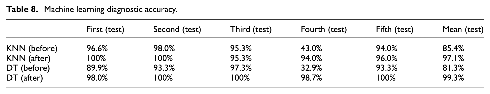
The results of the diagnostic tests are shown in Table 8. Before denoising, the above two classifier models had 1–2 diagnostic accuracy lower than 90% in five crossover experiments, and the accuracy of the models was below 50% in the fourth cross-test (the validation random number seed parameter values were not changed). After the noise reduction by the method in this paper, the diagnostic accuracy of all five cross-tests reached over 90%. The average diagnostic accuracy of KNN was improved from 85.4% to 97.1%; the average diagnostic accuracy of DT was improved from 81.3% to 99.3%. Therefore, the noise reduction preprocessing method applied to traditional machine learning in this paper has a good improvement on its diagnosis accuracy.

Table 8.

Machine learning diagnostic accuracy.

	First (test)	Second (test)	Third (test)	Fourth (test)	Fifth (test)	Mean (test)
KNN (before)	96.6%	98.0%	95.3%	43.0%	94.0%	85.4%
KNN (after)	100%	100%	95.3%	94.0%	96.0%	97.1%
DT (before)	89.9%	93.3%	97.3%	32.9%	93.3%	81.3%
DT (after)	98.0%	100%	100%	98.7%	100%	99.3%

Fault diagnosis based on deep learning

Unlike traditional machine learning fault diagnosis, deep learning adaptively extracts potential features of the signal and establishes a nonlinear mapping between features and fault types to achieve end-to-end fault diagnosis. The diagnostic test steps are as follows.

1. Data set division: similarly, 4096 data points were used for sample division, with a total of 744 samples. Randomly divide the training set (632), test set (112) according to the ratio of 8.5:1.5.

2. Deep learning models: the one-dimensional convolutional neural network Wdcnn ³⁸ model and the two-dimensional convolutional network ResNet34 ³⁹ model were used for fault diagnosis experiments, respectively, and the hyperparameters of each model are shown in Table 9, and the number of layers in the table represents: the number of convolutional layers + pooling layers, and the BN layers and Dropout layers added in the model are not shown. The training steps for each model are shown as follows.

Table 9.

Hyperparameters of deep learning models.

Parameter	Wdcnn	ResNet34
Number of layers	5	32
Number of fully connected layers	2	2
Number of learning parameter	85,571 bytes	21,286,211 bytes
Batch size	32	16
Betas	(0.9, 0.99)	(0.9, 0.99)
Learning rate	0.0001	0.0001
Weight decay	0.01	0.01
Momentum	0.1	0.1
Epoch	50	50
Loss function	Cross-entropy	Cross-entropy
Optimizer	Adam	Adam

Specific steps for model training:

① Similarly, the fivefold cross-validation method is used to divide the training set into five parts equally, and one part of each training is taken as the validation set and the other four parts as the training set. And ensure the consistency of data distribution.② The total number of iterations per training is set to 50 (the termination condition of each training). After each iteration is completed, the accuracy and loss values of the current model are calculated by inputting the validation set in order to observe the iterative process of the model. Fifty iterations are completed and the accuracy of the model is tested with the test set.③ The diagnostic accuracy of the five test sets is obtained after five training sessions, and the mean value is taken as the final diagnostic accuracy of the model.

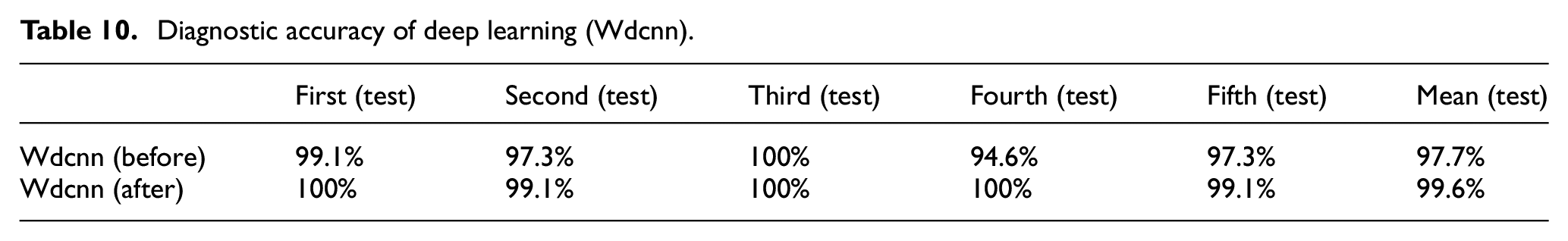
Based on the Wdcnn model diagnosis test, the timing characteristics of the vibration signal are directly used as the network input, and the diagnostic accuracy results of the test set are shown in Table 10. Before noise reduction, the diagnostic accuracy of the model fluctuated above and below 97%, and the average diagnostic accuracy was 97.7%; after noise reduction by the method of this paper, the diagnostic accuracy was stabilized above 99%, and the average diagnostic accuracy was improved to 99.6%.

Table 10.

Diagnostic accuracy of deep learning (Wdcnn).

	First (test)	Second (test)	Third (test)	Fourth (test)	Fifth (test)	Mean (test)
Wdcnn (before)	99.1%	97.3%	100%	94.6%	97.3%	97.7%
Wdcnn (after)	100%	99.1%	100%	100%	99.1%	99.6%

Taking the first cross-validation test as an example, the accuracy of the validation set before and after noise reduction is shown in Figure 9. In the initial iteration, the network training converges slowly and the accuracy of the validation set is low, and the network gradually converges with the updating of the weight parameters. The diagnostic accuracy of the validation set before noise reduction increases slowly after the 15th iteration and reaches 100% at the 30th iteration; the diagnostic accuracy of the validation set after noise reduction by this method gradually increases after the 10th iteration and stabilizes at 100% at the 20th iteration. Therefore, the noise reduction pre-processing method in this paper can effectively enhance the expression ability of fault features, reduce the time required for model training, and effectively improve the diagnosis efficiency and accuracy.

Figure 9.

Iterative graph of – validation set accuracy (Wdcnn).

Based on the ResNet34 model diagnosis test, the vibration signal is firstly transformed into a time-frequency diagram by using the “Morlet” wavelet base, ⁴⁰ as shown in Figure 10. Under the interference of noise, the signal contains more noise frequency components, and the color of the time-frequency diagram varies in shades and distribution, which cannot accurately express the time-frequency information of the fault. After the noise reduction process in this paper, the noisy frequency components are removed, leaving the time-frequency information of the regular distribution of the fault characteristics.

Figure 10.

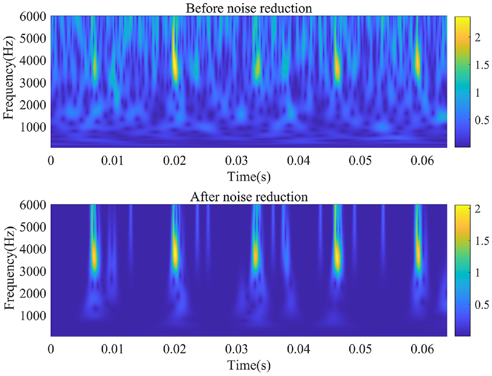
Time-frequency diagram – before and after noise reduction.

The results of the diagnostic accuracy of the test set are shown in Table 11. Before noise reduction, the diagnostic accuracy of the model fluctuated above and below 97%, and the average diagnostic accuracy was 97.3%; after noise reduction by the method of this paper, the diagnostic accuracy was stabilized above 99.1%, and the average diagnostic accuracy was improved to 99.8%.

Table 11.

Diagnostic accuracy of deep learning (ResNet34).

	First (test)	Second (test)	Third (test)	Fourth (test)	Fifth (test)	Mean (test)
ResNet34 (before)	95.5%	97.3%	96.4%	100%	97.3%	97.3%
ResNet34 (after)	100%	100%	99.1%	100%	100%	99.8%

Taking the first cross-validation test as an example, the accuracy iterations of the validation set before and after noise reduction are shown in Figure 11. With the increase of the number of iterations, the diagnostic accuracy of the validation set before noise reduction fluctuates continuously above and below 97%, and the diagnostic accuracy of the validation set after noise reduction is basically stable at 100%. Therefore, the noise reduction pre-processing method in this paper can effectively improve the diagnostic accuracy and stability of the improved model.

Figure 11.

Iterative graph of – validation set accuracy (ResNet34).

In summary, the noise reduction preprocessing method in this paper can enhance the expression of fault information in the signal, thus improving the diagnostic accuracy of traditional machine learning and deep learning-based fault diagnosis methods. At the same time, it is also valuable for improving the diagnostic efficiency and stability of deep learning fault diagnosis methods.

Conclusion

To deal with the problem that the rolling bearing fault vibration signal is weak and difficult to be extracted under the noise interference caused by mechanical equipment and surrounding environment, etc. A rolling bearing fault diagnosis method based on improved VMD-adaptive wavelet threshold joint noise reduction is proposed, and the main conclusions are as follows.

1. A dual determination criterion of sample entropy and correlation coefficient is constructed to screen the modal components of the decomposition. It effectively removes the noise components and avoids the one-sidedness of IMFs selected by a single indicator.

2. An adaptive wavelet threshold function is proposed. It is capable of adaptively adjusting the noise reduction form according to the noise content of the components, and thus has a certain degree of adaptivity. It solves the problems of excessive noise reduction and poor noise reduction of traditional wavelet thresholding, semi-soft thresholding, and other fixed forms of noise reduction algorithms.

3. Through simulation experiments and fault diagnosis experiments, the noise reduction preprocessing method proposed in this paper can effectively eliminate the noise components mixed in the signal, and enhance the expression ability of the features. It has good robustness, and a certain improvement on the diagnosis accuracy of the traditional machine learning and deep learning based diagnosis methods. Therefore, the noise reduction preprocessing method proposed in this paper has potential and value when applied to the research of rolling bearing fault diagnosis.