
Abstract
The high-speed maglev train will be subjected to extremely obvious aerodynamic load and instantaneous aerodynamic impact during passing another train, which brings significant challenges to the train’s suspension stability and safe operation. It’s necessary to consider the influence of aerodynamic load and shock waves in the design of suspension control algorithms. Traditional proportion integration differentiation (PID) control cannot follow the change of vehicle parameters or external disturbance, which is easy to cause suspension fluctuation and instability. To improve the suspension stability and vibration suppression of the high-speed maglev train under aerodynamic load and impact, we design a siding mode controller introducing the primary suspension’s deformation to replace the aerodynamic load on the electromagnet. Furthermore, we establish the train’s dynamic simulation model with three vehicles and compare the designed controller and the PID controller for their performance in controlling the model suspension stability in the presence of the train operating in open air. Simulation results show that the sliding mode control (SMC) method proposed in this paper can effectively restrain the electromagnet fluctuation of the train under aerodynamic loads.
Keywords
Introduction
The speed of the wheel-rail train is gradually increasing to meet the needs of people, but the limit of wheel-rail adhesion will restrict the increase of speed. The maglev train suspends around the track, avoiding contact between the track and the vehicle. Therefore, it overcomes the disadvantage of excessive friction caused by the direct connection between the wheel and rail of the traditional vehicle. Compared with the conventional vehicle, it has the advantages of low energy consumption, small environmental impact, low noise, less maintenance, and strong climbing ability. In recent years, the maglev train has made significant progress. China’s maglev system at 600 km/h was launched on July 20, 2021. 1 Since the aerodynamic load is directly proportional to the square of the speed, the aerodynamic load must increase sharply with the increase of the speed, which will impact the stability of the train. 2 We get through a numerical calculation based on the Shanghai maglev demonstration line. Results show that the tail car’s average aerodynamic and instantaneous lift can reach 10 and 14 tons when the train passes another train at 600 km/h. Because electromagnetic system (EMS) high-speed maglev vehicle relies on vertical electromagnetic force to achieve stable suspension, such a sizeable aerodynamic lift and impact will significantly influence the suspension stability and safety of the train. Kwon et al. 3 conducted a numerical simulation on the response of the maglev train passing through the suspension bridge under gust wind. They found that the ride comfort of the maglev vehicle is poor due to the low-frequency vibration of the car caused by the bridge and turbulence wind. Yau 4 considered the aerodynamic load caused by unstable airflow and calculated the response of the vehicle-guideway coupling system; the results show that the aerodynamic load may cause the significant gap amplification of the high-speed maglev train. Wu and Shi 5 completed the numerical analysis of the dynamic response of the maglev vehicle body under the wind field. Moreover, Liu and Tian 6 simulated the lateral vibration response of the maglev vehicle when it passes in open air. Takizawa 7 studied the comfort of the MLX01 maglev train when it operates at 500 km/h.
For the EMS maglev train, due to the inherent instability of the electromagnetic suspension system, it is necessary to exert control on the approach to maintain stable operation; therefore, the response of the EMS maglev train under external disturbance is closely related to the control algorithm. At present, the control algorithm of the high-speed maglev train is still based on PID control, which realizes feedback control by calculating the acceleration of the electromagnet and the difference between the actual gap and rated gap.8,9 However, PID control does not involve the vehicle system parameters and external disturbance; the algorithm will not change with the load on the train, which is easy cause the fluctuation and instability of the suspension gap. Common state feedback control is challenging to meet the control requirements, so algorithms such as neural network control,10,11 genetic algorithm control,12,13 and sliding mode control 14 have been applied to the electromagnetic suspension system. Among them, sliding mode control has attracted the attention of many scholars because of its strong robustness and anti-disturbance.
Molero et al. 15 used the sliding mode control to the magnetic suspension ball to control the position of the nonlinear system composed of the iron ball and the electromagnetic coil. Wang et al. 16 analyzed a single-axis magnetic suspension system and designed an adaptive sliding mode control that could deal with unknown parameters to complete the guidance and positioning of the system. Bandal and Vernekar 17 developed a sliding mode controller for position control of electromagnets based on the concept of proportional-integral switching surface. In addition, they compared the sliding mode controller with the feedback linearization controller and found that the sliding mode controller’s effect is more effective. Yang et al. 18 developed a new dynamic sliding surface by combining the disturbance estimation value and its high-order derivative information and proposed a continuous dynamic sliding mode control (CDSMC) method used in the suspension control system. Benomair et al. 19 proposed a fuzzy sliding mode controller (FSMC), which can estimate the unmeasured state using a nonlinear observer. To study the influence of air resistance on the dynamic response of the maglev train, Gao et al. 20 proposed an operation control method based on sliding mode periodic adaptive learning control (SM-PALC) to reduce position error and improve the robustness of the control system. Dourla et al. 14 designed a dynamic sliding mode controller by controlling the current through the electromagnetic coil. Chen et al. 21 introduced sliding mode control into the research of flexible track of maglev train, and designed the sliding mode adaptive state feedback controller of the maglev system, then compared it with the PID controller. Results show that the controller can guarantee faster dynamic response and stronger robustness when considering flexible orbit disturbance. Xu et al. 22 proposed a hybrid flux density observer based on current and voltage feedback, then designed an adaptive sliding mode controller to reduce the parameter uncertainty and upper bound of disturbance.
In the dynamic process, sliding mode control can constantly change according to the current state of the system, force the system to move according to the preset state trajectory of “sliding mode,” and overcome the uncertainty of the system. Because the sliding mode is independent of parameters and disturbances, it has the advantages of fast response, insensitivity to parameter changes and disturbances, no need for online identification of the system, and simple physical implementation. To overcome the influence of the aerodynamic load and suppress the vibration of the electromagnet during the train operation, we design the suspension controller of the maglev train based on the sliding mode control technology. When subjected to aerodynamic load and impact, the sliding mode controller can change the structure to maintain the stability of the system. However, it’s impossible to measure the aerodynamic load on the maglev train in real-time during the operation and there is no scholar has given a solution on introducing the influence of aerodynamic disturbance to the controller conveniently and effectively. Given that aerodynamic load and impact will cause the car-body of the train to vibrate, and the vibration of the car-body will be transmitted to the electromagnet through the secondary suspension, the maglev frame, and the primary suspension, the fluctuation of primary suspension force can be regarded as the disturbance of aerodynamic load to the electromagnetic suspension system. Therefore, considering the influence of primary suspension force disturbance on the suspension system, we derive a sliding mode controller with the impact of primary suspension deformation disturbance. Furthermore, we compare the designed sliding mode controller and a PID controller for their performance in the presence of operating in open air by simulation. Simulation results show that compared with the PID controller, the sliding mode controller can perform better in restraining the vibration response of the maglev train under aerodynamic load. Moreover, the load on the train can be reflected in the control process by considering the primary suspension deformation disturbance in the sliding mode controller so that the suspension gap of the train can be controlled and adjusted more effectively.
Single-point suspension model
A single-point two-stage suspension model is shown in Figure 1.

Schematic diagram of the single-point two-stage suspension system.
In Figure 1, z is the distance between the electromagnet and the guideway (i.e., the actual gap). When the train is operating, the equilibrium suspension gap between the electromagnet and the guideway is z0 and the purpose of controlling the train is to make it run according to the target track. In addition, Δz is the deviation between the actual gap z and the ideal gap z0, namely Δz = z − z0.
The vertical motion equation of the electromagnet can be written as:

Where m is the mass of the electromagnet, F (i, z) is the electromagnetic suspension force between the electromagnet and the track, fst(t) represents the balance value, and funst(t) is the fluctuation of the primary suspension force.
The single-point suspension force is23,24:

In (2), μ0 is the air permeability, A is the effective area of the electromagnet, N is the turns of the coil, z is the suspension gap, and i is the current of the coil on the electromagnet.
The maglev train directly adjusts the current in the electromagnet through the suspension control unit. The dynamic equation can be written as follows:
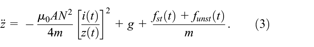
Let

Set

The state equation is rewritten as:

or

Where
Design of sliding mode controller
Design of sliding surface
The switching surface s(x) = 0 is determined to ensure the asymptotic stability and great dynamic characteristics of the dynamic system on the sliding surface.
Define tracking error

The switching function of the system is designed as:

Where cd and c are undetermined constants; z0 is the equilibrium suspension gap.
To guarantee the asymptotic stability on the sliding surface of the system, it is necessary to meet c > 0.
Design of sliding mode law
The design of the sliding mode control law needs to meet:
the system state can enter the sliding mode state from any initial point;
the system can be stably and reliably maintained on the sliding mode surface after entering the sliding mode state.
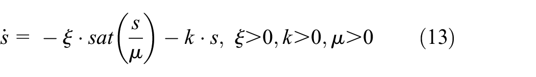
The law of convergence mainly has the constant rate of convergence, the exponential rate of convergence, and the power rate of convergence. The exponential reaching law can effectively reduce buffeting vibration in the form of:

Where ξ is the gain coefficient and k is the approach rate. They are all undetermined constants.
According to (10), we can get:

The electromagnet is expected to levitate stably at 10 mm, so z0 = 10 mm,

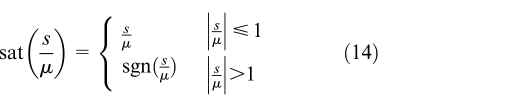
Because the moving point of the system still has velocity when it reaches the switching surface, it will continue to pass through the switching surface under inertia. The moving point in the sliding mode will be accompanied by high-frequency vibration, thus forming buffeting vibration. In exponential approach law (10) “
Where μ is an undetermined constant, “sat” is a saturation function whose expression is:
The control law of the system can ultimately be determined as:
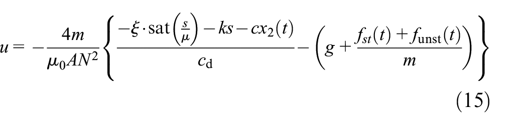
The variation term funst of the primary suspension load is included in the sliding mode control law (16). In this way, the variable structure characteristics of the sliding mode controller can be well-reflected. In other words, the controller can continuously change according to the aerodynamic load disturbance of the vehicle and force the suspension system to move according to the state trajectory of the predetermined “sliding mode” to overcome the uncertainty of the maglev train.
As shown in Figure 1, the vibration of the car-body under aerodynamic load will be successively transmitted to the electromagnet through the secondary suspension, maglev frame, and primary suspension. So, the fluctuation of primary suspension force can be regarded as the disturbance of aerodynamic load or vehicle body vibration to the electromagnetic suspension system. To adjust the parameters of the controller, we use (16) to express the variation of the primary suspension force, in which ΔZprimary is the deformation of the primary suspension spring and Kpri is an adjustable parameter.

The dynamic model of the maglev train with three vehicles
The main components of each maglev train include the car-body, four suspension frames, electromagnets installed on the suspension frame, and so on. The connection between electromagnet and suspension frame is primary suspension, and the connection between suspension frame and the car-body is secondary suspension. The primary suspension is made of rubber springs, and the secondary suspension is relatively complex, including the pillow beam, air spring, and pendel. Because the electromagnet is installed on the suspension frame, the suspension frame plays the role of transferring the suspension force, traction force, braking, and guiding force to the car-body through suspension. This paper considers the main components of the actual train mentioned above when modeling the dynamics of the maglev train. The dynamic model of the single-vehicle TR08 maglev train is shown in Figure 2. Each vehicle is mainly composed of the following parts: car-body (1 piece), frame (4 pieces), anti-roll/pillow beam (8 pairs), pendel (8 pairs), traction pull rod (4 pieces), suspension magnet (8 pairs for intermediate vehicle and 7.5 pairs for lead vehicle), brake magnet (1 pair), guide magnet (6 pairs), air spring (8 pairs), car-body transverse elastic holder or rubber spring, traction/suspension electromagnet and suspension frame unit support (16 pairs for intermediate vehicle and 15 pairs for lead vehicle), brake electromagnet support, etc.

Vehicle dynamics model.
In the dynamic modeling, each suspension frame is simplified as two semi-maglev frames, because the suspension frame is connected by two C-shaped structures and the longitudinal beam connected in the middle has large flexible deformation. Other parts are considered rigid bodies, and their elastic deformations can be ignored. In the dynamic model of the train, the suspension structure of the vehicle reflects the independence of stiffness in all directions: the vertical, transverse, and longitudinal traction of the secondary system are provided by the air spring, boom (pendel), and traction device, respectively. The primary suspension is independently provided by supporting rubber parts or arthrosis structures of the traction electromagnet and the guide (including brakes, replacements) electromagnet. Suspension electromagnetic force realizes active control through the control system to levitate the vehicle, and the track is coupled with the train through this electromagnetic force.
Based on the dynamic model established with the TR08 train as the reference in Figure 2, we use the multi-body dynamics software SIMPACK to develop a maglev train model with three vehicles, shown in Figure 3. The position of electromagnets on each vehicle is marked in the figure.

The maglev train model with three vehicles of TR08 maglev train.
In this paper, the train was controlled dispersedly so that the design of the whole vehicle suspension control system can be completed by designing the single electromagnet suspension control system, simplified. Each electromagnet of the maglev train has 12 magnetic poles, as shown in Figure 4. Every six magnetic poles is a group, so each electromagnet has two independent controls. However, the two groups of magnets in the same electromagnet module are integrated and the adjacent electromagnets are connected through the magnetic levitation frame, so the electromagnet movement under the mutually independent control system affects each other.

Magnetic pole distribution on a single electromagnet.
This paper presents the single-channel sliding mode control (SMC) suspension control scheme, as shown in Figure 5. In the control model, x2(t) is calculated by integrating the measured acceleration and the fluctuation of the primary force fst can be measured by the simulation model.
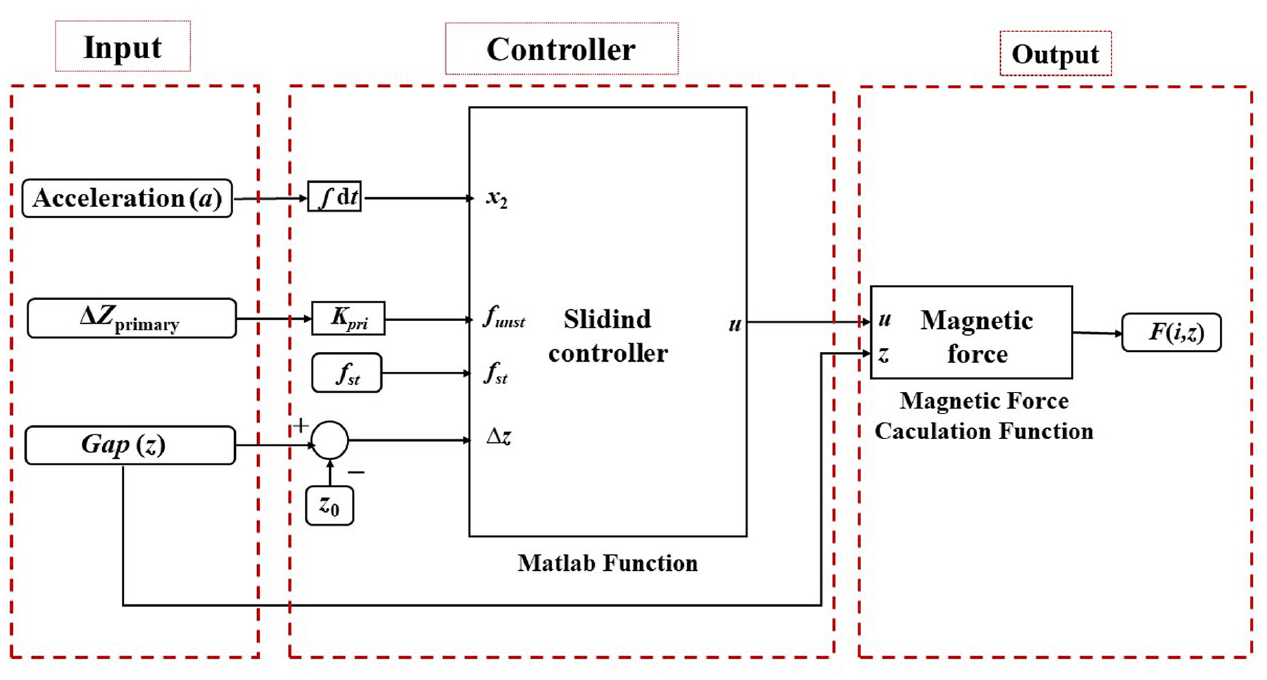
Single-channel SMC suspension control system model.
The expression of the control model is:

The parameters of the SMC controller are set to c = 100, cd = 1, ξ = 20, k = 80, Kpri = −2 × 10⁷/6. If Kpri = 0 in (17), it is just an ordinary SMC.
Based on the dynamic simulation model and the suspension control model of the train, the data transmission between the multi-body dynamic model and the control model is realized through the SIMAT interface in MATLAB, as shown in Figure 6. This interface can realize the coupling simulation between multi-body dynamics and suspension control of the train. Each single-channel control unit is composed of input, controller, and output. The vehicle multi-body dynamic model transmits the measured primary suspension force fluctuation, electromagnet suspension gap, and acceleration to the controller. The controller calculates these data to obtain the desired current value, calculates the electromagnetic suspension force, and returns the force to the vehicle’s multi-body dynamic model.

SIMAT interface.
At the same time, to demonstrate the control effect of the proposed SMC controller, this paper also used the proportion integration differentiation (PID) control algorithm as the comparison. PID control algorithm linearly combines the proportion (P), integral (I), and differential (D) of the suspension gap deviation into control quantities to correct the deviation of the controlled object, so as to make the suspension system reach a stable state. The single-channel PID controller is shown in Figure 7.

Single-channel PID suspension control system model.
Each single-channel PID controller unit comprises the input, controller, and output. The estimated velocity value in the state observer is a weighted combination of the suspension gap and its velocity and acceleration. Each control unit receives the electromagnet suspension gap and acceleration input from the vehicle dynamics model. These signals are filtered and observed through the Simulink, and the electromagnetic suspension force is calculated by the controller and fed back to the dynamic simulation module. In PID control, the proportional gain coefficient, the integral gain coefficient, and the differential gain coefficient are set to K1 = 7000, K2 = 200, K3 = 0.5, and K4 = 1000.
Analysis of train response under aerodynamic load
Aerodynamic load data
Simulation calculation considers the aerodynamic lateral force, lift force, rolling moment, pitching moment, and yaw moment on the train. Based on the Computational Fluid Dynamic (CFD) method, we simulate these loads of the train operating in open air at 300, 400, and 500 km/h. Under different operating speeds, the variation curve of the aerodynamic load acting on the train is basically the same. Still, the load amplitude will increase with the increase in train speed. The aerodynamic loads on the train when the train operates at 500 km/h are shown in Figure 8. The aerodynamic moment results from taking the center of mass of the car-body as the moment point. The blue, green, and orange solid lines represent the aerodynamic load on the head, middle, and tail car during train operations. The range between the two black dashed lines in the figure represents the passing stage, which means that the trains running in the opposite direction meet with each other. The curves of other parts are the aerodynamic loads when the train operates alone. Obviously, the tail train receives the most significant aerodynamic load when the train is running, followed by the head car, and the middle car is more petite. It is noted that the aerodynamic load fluctuates obviously in the train passing stage.

Aerodynamic load when train operates at 500 km/h: (a) lateral force, (b) lift force, (c) rolling moment, (d) pitching moment, and (e) yaw moment.
We apply the above aerodynamic loads to the vehicle centroid in the dynamic model and carry out the motion simulation of the maglev train under aerodynamic loads. Moreover, we compare the dynamic response of the train using the PID controller, traditional SMC controller, and sliding mode control considering primary suspension disturbance (SMC_P).
Car-body response analysis
This section analyzes the calculation results of the car-body (yellow part in Figure 2) response of the maglev train, including the vertical acceleration and displacement. We can use these results to judge the stability and comfort of the train during operation.
The Sperling ride index reflects the response results of the vertical acceleration of the car-body. GB5598-85 specification points out that the Sperling ride index can be used to evaluate the stability of trains during operation and formulates the dynamic performance evaluation of railway vehicles based on the Sperling ride index method. 25 According to the calculated index value, riding comfort can be divided into different grades. When the Sperling ride index is less than 2.5, it can be considered excellent.
Generally, the calculation formula of Sperling ride index value of single frequency response is:
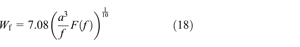
Where Wf is the Sperling ride index value, a is the amplitude of acceleration, F(f) is the correction factor of frequency, and f is the frequency. When the vehicle response is composed of multiple frequency components, the total Sperling ride comfort index W is:

The results of the Sperling ride index of the train operating at different speeds in open air under aerodynamic loads are shown in Table 1.
Comparison of the vertical Sperling ride index (Unit: 1).
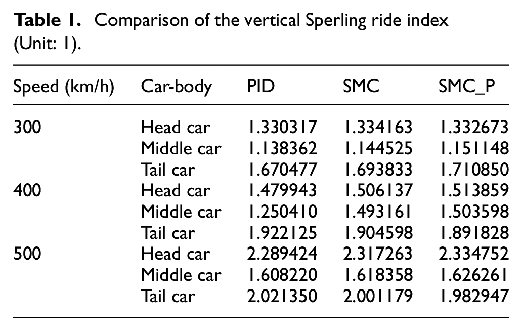
It is apparent that the Sperling ride index of the train gradually increases with the increase of speed. The results about the Sperling ride index are all less than 2.5 in the case of PID controller, traditional SMC controller, and sliding mode with primary suspension force disturbance (SMC_P), which means the train has excellent stability.
Table 2 shows the heave motion amplitudes of the car-body using three controllers when the train operates in open air at different speeds. The head train’s vertical vibration amplitude is the smallest, and the tail train is the largest at different rates. The vibration amplitude of the train increases gradually with the rise of the speed. Under the three controllers, the vertical vibration amplitude of the car-body is relatively close and the maximum value is 95 mm. Compared with the height of the car-body of 3 m, the displacement fluctuation is smaller and the comfort is excellent.
Vibration amplitudes of the car-body (Unit: mm).
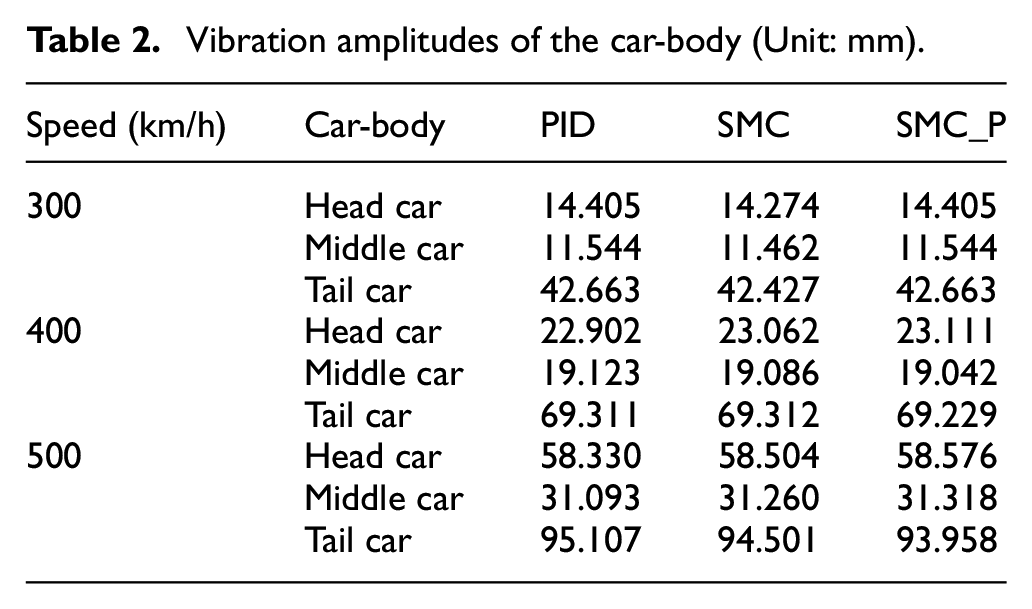
The motion of the car-body is mainly affected by the aerodynamic load, so the Sperling ride index and vertical motion amplitude of the car-body under the three control strategies have little difference.
Suspension gap response of electromagnet
In addition to the dynamic response of the car-body, the suspension gap fluctuation is also a major concern of the maglev train. In the dynamic model of the maglev train, 23 electromagnets are installed on the left and right sides respectively and Figure 3 shows the distribution of these electromagnets. Figures 9 to 11 show the fluctuation curves of the electromagnet suspension gap on the right at positions H1, M1, M9, and T7 when the train operates at different speeds. The black dotted line corresponds to the period when the two trains pass each other.

Electromagnet gap fluctuation when the train operates at 300 km/h (negative ordinate represents the upward movement of the electromagnet): (a) the first electromagnet of the head car, (b) electromagnet between head car and middle car, (c) electromagnet between middle car and tail car, (d) the last electromagnet of the tail car.

Electromagnet gap fluctuation when the train operates at 400 km/h (negative ordinate represents the upward movement of the electromagnet): (a) the first electromagnet of the head car, (b) electromagnet between head car and middle car, (c) electromagnet between middle car and tail car, and (d) the last electromagnet of the tail car.

Electromagnet gap fluctuation when the train operates at 500 km/h (negative ordinate represents the upward movement of the electromagnet): (a) the first electromagnet of the head car, (b) electromagnet between head car and middle car, (c) electromagnet between middle car and tail car, (d) the last electromagnet of the tail car.
Using the sliding mode controller considering the primary suspension deformation disturbance designed in this paper, the gap fluctuation values of the electromagnet are smaller than those using the traditional SMC controller. Compared with using the PID controller, it has more excellent performance and better suspension stability.
Table 3 shows the average values of the electromagnetic suspension gap amplitude of the head, middle, and tail car when the train operates in open air at different speeds. Obviously, the fluctuation amplitude of the suspension gap of the train using sliding mode control considering the disturbance of the primary force is significantly reduced at different speeds compared with using PID controller and traditional SMC controller.
Average amplitudes of the electromagnet suspension gap (Unit: mm).

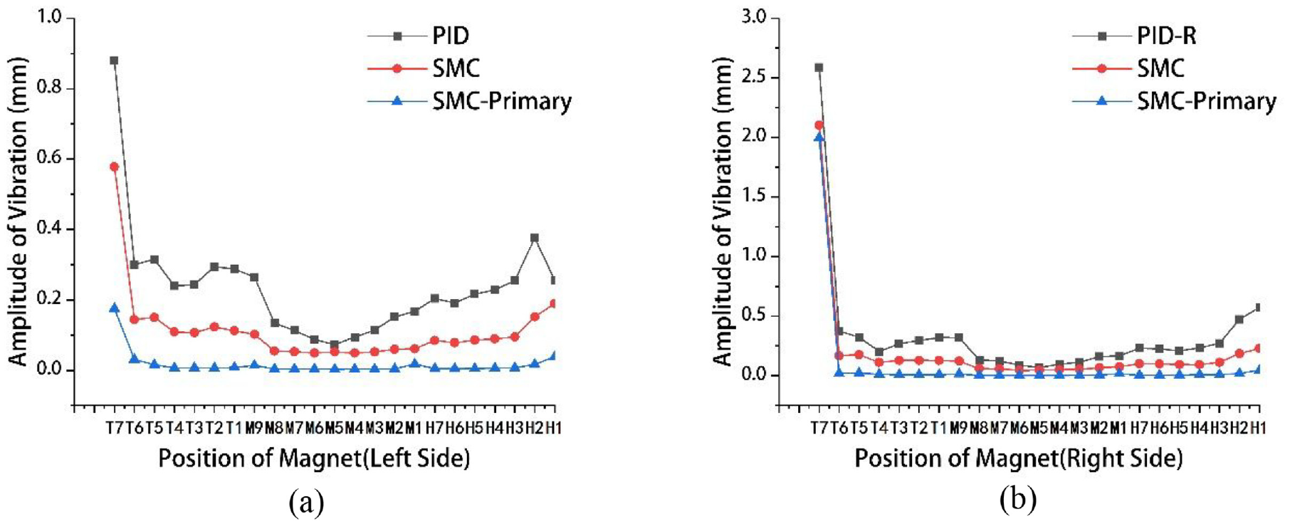
To more specifically illustrate the fluctuation of the suspension gap of electromagnets under using three kinds of the controller, Figures 12 to 14 show the amplitudes of the gap fluctuation, including all electromagnets of the train. Under the influence of roll moment in aerodynamic load, the fluctuation of the electromagnet suspension gap on both sides of the train will be slightly different. It can be seen that under the action of the controller designed in this paper, the suspension gap amplitude of the whole train at 300 km/h is less than 0.1 mm, the suspension gap amplitude at 400 km/h is less than 0.2 mm, and the suspension gap amplitude at 500 km/h is less than 2 mm, showing good suspension stability.

Amplitude distribution of the suspension gap when the train operates at 300 km/h: (a) electromagnets on the left side of the train and (b) electromagnets on the right side of the train.

Amplitude distribution of the suspension gap when the train operates at 400 km/h: (a) electromagnets on the left side of the train and (b) electromagnets on the right side of the train.
Amplitude distribution of the suspension gap when the train operates at 500 km/h: (a) electromagnets on the left side of the train and (b) electromagnets on the right side of the train.
Take the train operating at 300 km/h as an example. At position H1 of the head car, the gap fluctuation amplitude of the suspension gap is 0.14505 mm under the PID controller and 0.06786 mm under the traditional SMC controller. The amplitude is 0.01384 mm under the sliding mode controller designed in this paper, which is reduced by 90.49% compared with the PID controller and 79.61% compared with the traditional SMC controller. At the position T7 of the last electromagnet of the tail car, the fluctuation amplitude is 0.51499 and 0.22301 mm under PID and SMC controller. The amplitude of the gap fluctuation is 0.03761 mm under the controller proposed in this paper, which is 92.70% less than that of the PID controller and 83.14% less than that of the traditional SMC controller.
Discussion
It is found that when the train is running at high speed, the aerodynamic load of the head car and the tail car is significantly greater than that of the middle car, especially the electromagnet suspension gap at the end of the tail car fluctuates the most, which is prone to suspension instability.
Given this conclusion, we suggest: due to the difference in fluctuations of different electromagnets caused by the uneven distribution of aerodynamic load, the following measures can be tried to improve:
The uneven distribution of aerodynamic force can be improved by optimizing the aerodynamic shape of the train;
The control strategy of each suspension control unit is unified at present. In the later stage, we can try to use different control strategies for different control units and adopt a better control strategy for the electromagnet control units at the head and tail of the train.
It can also change the parameters of the primary suspension and secondary suspension of the head and tail position of the maglev train, so as to reduce vibration amplitude by changing the dynamic system characteristic parameters of the electromagnet.
Conclusion
In this paper, we transform the influence of aerodynamic load on electromagnet into the disturbance of primary suspension force, then design a sliding mode controller considering the disturbance of primary suspension force. Furthermore, we establish the dynamic simulation model of the high-speed maglev train with three vehicles to calculate the dynamic response of the train runs and passes with another train in open air. It is proved that under the controller’s action designed in this paper, the dynamic responses of train body displacement, Sperling ride index, and suspension gap fluctuation meet the requirements of train operation. Then, by comparing with PID and traditional SMC controllers, it is found that under the sliding mode control considering the disturbance of primary suspension force, the electromagnet fluctuation amplitude at each position of the train is significantly reduced, which proves that the controller proposed in this paper can effectively suppress the electromagnet fluctuation under aerodynamic load. This study can provide a reference for the suspension control optimization of the maglev train under aerodynamic conditions.
Footnotes
Handling Editor: Chenhui Liang
Author contributions
(1) Mengjuan Liu: The reasons she was listed as the author of this article are: (a) Methodology: She built the model and carried out the numerical calculation; (b) Writing – original draft preparation: Mengjuan Liu wrote and revised the article; (c) Her contributions to this article also include: Data curation, formal analysis, and visualization. (2) Han Wu: The reasons for Han Wu was listed in the author list are as follows: (a) Conceptualization: Han Wu constructed the main research purpose of the article; (b) Funding acquisition: This project was supported by the National Natural Science Foundation of China (Grants 51805522, 11672306, and 51490673), and Prof. Wu is the recipient of the fund; (c) His contributions to this article also include: Supervision and Writing – review & editing. (3) Junqi Xu: The reasons Junqi Xu was listed in the author list are as follows: (a) Funding acquisition: This project was supported by the Key Laboratory of Railway Industry of maglev Technology (TJU) and the National Railway Administration of PRC(KLOMT04), and Prof. Xu is the recipient of the fund; (b) Junqi Xu made important contributions to the revision of the manuscript including but not limited to: Data curation, Writing – review & editing, and supervision. (4) Xiaohui Zeng: The reasons Xiaohui Zeng was listed in the author list are as follows: (a) Funding acquisition: This project was supported by the open fund of the State Key Laboratory of Coastal and Offshore Engineering, Dalian University of Technology (Grant LP21V1), and Prof. Zeng is the recipient of the fund; (b) Supervision: Xiaohui Zeng supervised and directed the research. (5) Bo Yin: The reason Bo Yin was listed in the author list is as follows: Improve data: Bo Yin provided aerodynamic load data for the model. (6) Zhanzhou Hao: The reason Zhanzhou Hao was listed in the author list is as follows: Improve data: Zhanzhou Hao provided aerodynamic load data for the model.
Declaration of conflicting interests
The author(s) declared no potential conflicts of interest with respect to the research, authorship, and/or publication of this article.
Funding
The author(s) disclosed receipt of the following financial support for the research, authorship, and/or publication of this article: This project was supported by the Key Laboratory of Railway Industry of Maglev Technology (TJU), the National Railway Administration of P. R. C (KLOMT04); the National Natural Science Foundation of China (Grants 51805522, 11672306, and 51490673); the open fund of the State Key Laboratory of Coastal and Offshore Engineering, Dalian University of Technology (Grant LP21V1).