Sage Journals: Discover world-class research

Abstract

The high noise and low energy characteristics of the raw signals collected by sensors make the signal features weak and difficult to train. The purpose of this paper is to enhance the fault features of abnormal signals using the hierarchical feature enhancement method (HFE) which contains three layers. In the first layer, the signals are decomposed into multiple modals estimated by a variational optimization problem. The modals we choose are used to reconstruct the signals to form a complex matrix used to extract features in the second layer. In the third layer, the feature signals are converted into two-dimensional space and then are input into the convolutional neural network (CNN) for fault diagnosis after HFE since CNN helps to mine deeper features and compute in parallel on a large scale. The experimental results effectively verify the performance of the HFE for enhancing the weak fault features and preventing noise interference. The signals analyzed by HFE used as input greatly improve the diagnosis ability of CNN. In addition, the ablation and comparison experiments are conducted which still show superiority.

Keywords

Hierarchical feature enhancement method (HFE)convolutional neural network (CNN)fault diagnosis

Introduction

Fault information will be reflected in the equipment through signals, and these fault messages often form abnormal signals that are difficult to monitor through external equipment. Indirect sensing methods diagnose faults by analyzing condition monitoring data collected via sensors including temperature, forces, vibration, and sound. Hence, indirect sensing methods are more practical while eliminating the need for manual inspection intervention making the detection process more efficient and less costly.¹ Fault diagnosis methods can be broadly divided into two categories: model-based methods and data-driven methods. Model-based methods measure process variables and estimate residuals based on the physical properties of the dynamic system.² Increasingly, a large amount of sensor data drives the development of data-driven methods. These approaches focus on the condition monitoring data which means no prior knowledge of the data distribution is required. It makes the data-driven approach more agreeable.³

Signals are constantly collected during operation to accumulate large amounts of historical data, making the data-driven approach increasingly accurate. Among those methods, the deep learning methods are widely used in recent years. Since a deep belief network is applied to fault detection,⁴ more and more scholars use the deep learning method for fault diagnosis. Since the data is generally one-dimensional, LSTM and GRU methods are commonly used for diagnosis. However, LSTM and GRU too rely on the current state. Meanwhile, the inability to process multiple temporal data in parallel makes LSTM and GRU increasingly disadvantageous in fault diagnosis.⁵ Compared with the situation, we found that it is the CNN model used in learning and analyzing that can be processed in parallel on a large scale, which has played a more and more essential role in image processing and signal processing as one of the most core algorithms in deep learning. CNN could reflect the characteristics of the signals on a deeper level and has great advantages in parameter sharing and sparse connectivity which accelerate the speed of computation and suppress the model overfitting.⁶ Hence, CNN is used more and more in signal processing which is helpful in diagnosis. However, although it can get good results in processing, one-dimensional CNN can be affected by noise easily.⁷ Then 2-D CNN is adopted since 2-D CNN has excellent feature extraction capability. Lu et al.⁸ combined the GA algorithm with 2-D CNN to make full use of 2-D CNN’s advantages in image processing. Therefore, converting one-dimensional fault signals into two-dimension is helpful for fault identification and classification.

The fault signals collected have the characteristics of non-linearity and non-stationarity.⁹ At the same time, due to the large noise generated during the operation of the equipment, the signals are easily drowned in the noise, making the fault features hard to extract and difficult to process. Although CNN has the ability to learn features by itself to some extent, features cannot be extracted well due to the fixed length of convolutional kernel length.⁵ To solve this problem, feature engineering is used as an auxiliary tool to better help CNN extract multi-domain features which means the features must be enhanced to draw the fault features better for fault diagnosis.

In the current research on signal feature enhancement, wavelet packet decomposition, empirical modal decomposition, and feature enhancement techniques based on entropy¹⁰ are mostly used. Among these three methods, wavelet packet decomposition¹¹ extracts the feature parameters of different frequency bands and weighted summation of the feature parameters to approximate and segment the original signal in detail. The empirical modal decomposition¹² decomposes the signal to estimate the similarity or cumulative contribution of each component to select representative features from the components. The representative method based on the principle of minimum entropy is the minimum entropy deconvolution¹³ which improves the fault feature extraction by enhancing the impact pulse of the signal. However, the effectiveness of wavelet packet decomposition is based on the selection of wavelet basis. Although it can provide a window that can adaptively adjust with the change of signal frequency, it improves time accuracy by sacrificing frequency accuracy. The empirical modal decomposition and the minimum entropy deconvolution¹⁴ suffer from edge effects leading to distortion.

Currently, most of the fault diagnosis is performed by enhancing the signals through the above-mentioned enhancement methods and then directly using the classification model SVM¹⁵ or combining it with the one-dimensional neural network models RNN, LSTM^16,17 to determine the faults. However, the deeper dimension signals are difficult to extract in one dimension and contain less information which makes models hard to diagnose.

In this paper, we propose a hierarchical feature enhancement method to enhance the features of fault signals. The HFE contains three layers including a signal denoising layer, a feature extraction layer, and a feature transforming layer. The signal denoising layer decomposes the signals into multiple modals to prevent noise interference. In the feature extraction layer, a Gaussian window function is added to the series to form a complex matrix for feature extraction. Then the feature transforming layer converts the feature sequence into polar coordinates from one-dimensional signals to two-dimensional space. CNN is used after the HFE to diagnose the faults.

The main innovations and contributions of our work are as follows:

The three layers in the HFE perform their respective duties. Fault features submerged in noise can be better extracted after the HFE.

The features extracted by the HFE can effectively resist the interference of noise, and can still better enhance the fault features in high noise scenarios.

Using the advantages of two-dimensional CNN in extracting high-dimensional features, the fault features are further enhanced, which greatly improves the accuracy of model diagnosis. At the same time, the experiments before and after the HFE show that the HFE plays a pivotal role in improving the accuracy of the model.

The remaining part of this paper is as follows: methods including HFE and CNN are introduced in Section 2. The experimental verification and ablation experiments are conducted and the results are also compared with other CNN-based feature enhancement methods in Section 3. Additionally, the conclusions and future work are summarized in Section 4.

Method

HFE method contains three layers which are the signal denoising layer, feature extraction layer, and feature transforming layer. HFE is used before CNN to separate the signals from noise and enhance the fault features. After HFE, signals have been converted into images that include enhanced features. And then those images are input into the CNN to train and test in order to realize the aim of fault diagnosis. The framework of the proposed signals HFE method for CNN-based fault diagnosis is shown in Figure 1.

Figure 1.

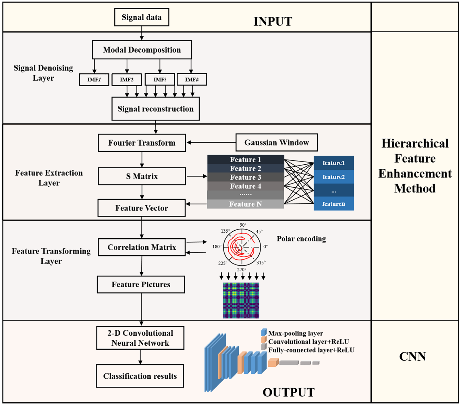
Flow chart of the framework.

Hierarchical feature enhancement method

Signal denoising layer

The fault features are buried in the noise and the feature information cannot be extracted well due to the fixed length of convolutional kernel length.⁵ HFE method is adopted to better enhance the features of signals with faults.

The signal denoising layer is mainly used to separate the signals from noise. The sampled signals contain noise which can be expressed as follows

f_{k} = f + η = \sum_{k} u_{k}

(1)

Where $η$ is noise and f is the signal after denoising. The modal decomposition is used to decompose the signals into several modals.

To find f, the regularization method is used.

min_{u_{k}} {‖ \sum_{k} u_{k} - f ‖_{2}^{2} + α \sum_{k} ‖ \partial_{t} f ‖_{2}^{2}}

(2)

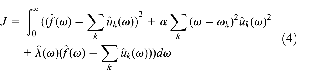
Where k is the mode number of decomposition. The first part of (2) is the cost function. Due to the non-uniqueness of the solution during decomposition, this problem is ill-posed. Therefore, the meaning of the second part is to add norms to eliminate ill-posed. L2 regular terms are added, $α$ is the penalty factor of L2 regular term, which is used to control the degree of penalty. The value is adjusted through the test set of subsequent experiments.¹⁸

Transform (2) to the frequency domain, and expand into a generalized function after that.

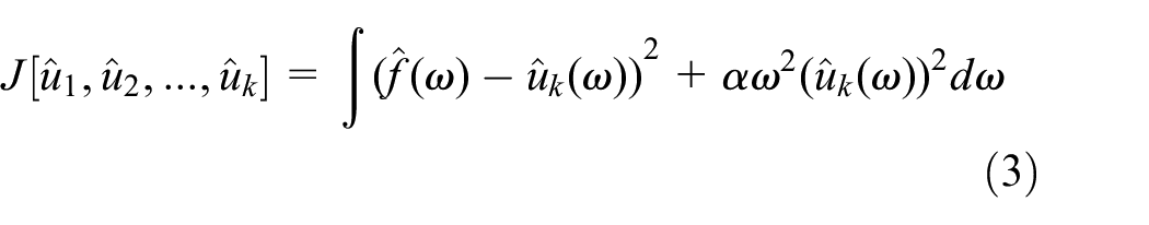
J [{\hat{u}}_{1}, {\hat{u}}_{2}, . . ., {\hat{u}}_{k}] = \int {(\hat{f} (ω) - {\hat{u}}_{k} (ω))}^{2} + α ω^{2} ({\hat{u}}_{k} (ω))^{2} d ω

(3)

Then the extreme value of can be found through (3).

To search for the optimal central frequency $ω_{k}$ , the alternating direction update technique is adopted after the update formula for ${\hat{u}}_{k}$ . Introduce the multiplier $λ$ thereby converting the constrained variational expression into an unconstrained variational expression.

\begin{matrix} J = \int_{0}^{\infty} ({(\hat{f} (ω) - \sum_{k} {\hat{u}}_{k} (ω))}^{2} + α \sum_{k} {(ω - ω_{k})}^{2} {\hat{u}}_{k} {(ω)}^{2} \\ + \hat{λ} (ω) (\hat{f} (ω) - \sum_{k} {\hat{u}}_{k} (ω))) d ω \end{matrix}

(4)

With the same progress, the final update equations are obtained as follows through calculating.

{\hat{u}}_{k} (ω) = \frac{\hat{f} (ω) - \sum_{i \neq k} {\hat{u}}_{i} (ω) + \frac{\hat{λ} (ω)}{2}}{1 + α {(ω - ω_{k})}^{2}}

(5)

ω_{k} = \frac{\int_{0}^{\infty} ω {| {\hat{u}}_{k} (ω) |}^{2} d ω}{\int_{0}^{\infty} {| {\hat{u}}_{k} (ω) |}^{2} d ω}

(6)

{\hat{λ}}^{n + 1} (ω) = {\hat{λ}}^{n} (ω) - τ (\hat{f} (ω) - \sum_{k} {\hat{u}}_{i} (ω))

(7)

The decomposition progress is based on variational mode decomposition.¹⁸ $τ$ is the noise tolerance, the default of it is 0.001. The iteration progress is stopped through precision ε which is small enough but bigger than 0.

\frac{\sum_{k} ‖ {\hat{u}}_{k}^{n + 1} - {\hat{u}}_{k}^{n} ‖_{2}^{2}}{‖ {\hat{u}}_{k}^{n + 1} ‖_{2}^{2}} < ε

(8)

Feature extraction layer

After performing the decomposition, the modal components to be retained are selected and the components to be rejected are rounded off. The signals after decomposition is $f_{k} - u$ , u is the modal to be removed. And then Fourier transform is performed on the signals after the signal denoising layer, and a Gaussian window function is added to the signals.

Since the height and width of the Gaussian window function vary with frequency, the drawbacks caused by the fixed window width are improved, allowing the transform to adjust the resolution.

F (f) = \int_{- \infty}^{\infty} (f_{k} - u) e^{- 2 i π ft} \frac{1}{σ \sqrt{2 π}} e^{\frac{t^{2}}{2 σ^{2}}} dt

(9)

Scale and translate the Gaussian window functions. Then the transform can be expressed as (10).

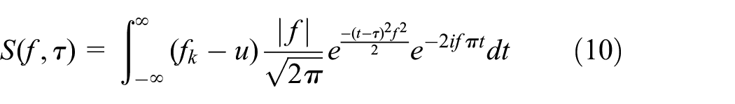
S (f, τ) = \int_{- \infty}^{\infty} (f_{k} - u) \frac{| f |}{\sqrt{2 π}} e^{\frac{- {(t - τ)}^{2} f^{2}}{2}} e^{- 2 if π t} dt

(10)

Where $σ = \frac{1}{| f |}$ .

Through (10), a two-dimensional matrix can be obtained, where the columns correspond to the sampling time, and the rows correspond to the frequency values. The matrix elements are complex values from which the amplitude and phase information can be extracted. The features representing the signals are extracted from the two-dimensional matrix, and the features extracted are then standardized as $F = [F_{1}, F_{2}, \dots, F_{n}]$ .¹⁹ Where $F_{i} = [F_{1 i}, F_{2 i}, . . ., F_{mi}]$ . Where n is the number of features extracted and m is the number of input signals.

F = [\begin{matrix} F_{11} & F_{12} & \dots & F_{1 n} \\ F_{21} & F_{22} & \dots & F_{2 n} \\ \dots & \dots & ⋱ & \dots \\ F_{m 1} & F_{m 2} & \dots & F_{mn} \end{matrix}]

(11)

Calculate its correlation coefficient matrix.

R = \frac{1}{m - 1} F^{'} F = [r_{ij}] = \frac{1}{m - 1} \sum_{k = 1}^{m} F_{ik} F_{jk} (i, j = 1, 2, . . ., n)

(12)

N non-negative eigenvalues are obtained through (12) which are $λ_{1} \geq λ_{2} \geq \dots λ_{N} \geq 0$ . A matrix is formed from the eigenvectors corresponding to the eigenvalues.

A = [\begin{matrix} ξ_{11} & ξ_{12} & \dots & ξ_{1 N} \\ ξ_{21} & ξ_{22} & \dots & ξ_{2 N} \\ \dots & \dots & ⋱ & \dots \\ ξ_{n 1} & ξ_{n 2} & \dots & ξ_{nN} \end{matrix}]

(13)

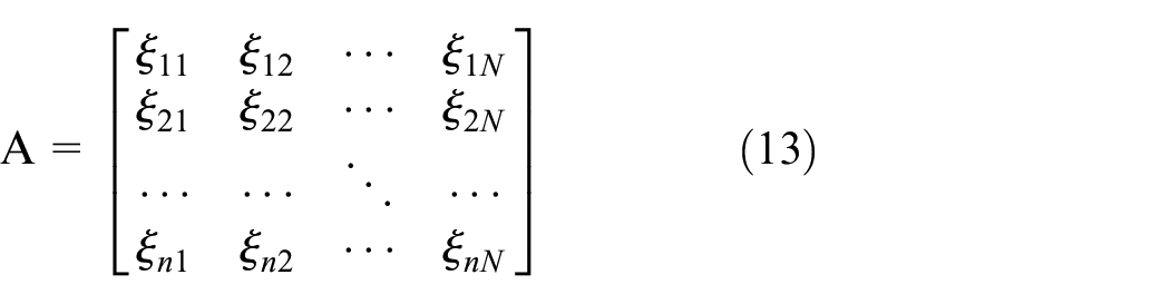
Each column in A is the eigenvector corresponding to $λ_{i}$ . Select the first k eigenvalues according contribution rate. And the calculation of contribution rate is:

\frac{λ_{i}}{\sum_{j = 1}^{k} λ_{j}}

(14)

The normalized F is multiplied by the eigenvector matrix corresponding to the selected eigenvalues to reconstruct the new features.

Feature transformation layer

Rearrange the regenerated features into a one-dimensional sequence to generate new eigenvectors.

Assume the series is $α = (α_{1}, α_{2}, . . ., α_{n})$ through feature extraction layer. And in the next feature transforming layer, signals are normalized first so that all values fall between [−1,1].

{\tilde{α}}_{i} = \frac{(α_{i} - max (α)) + (α_{i} - min (α))}{max (α) - min (α)}, - 1 \leq {\tilde{α}}_{i} \leq 1

(15)

Transform the sequence into polar coordinates after normalization.²⁰

{\begin{matrix} φ = \arccos ({\tilde{α}}_{i}) \\ r = \frac{t_{i}}{N}, t_{i} \in N \end{matrix}

(16)

Where $t_{i}$ is time stamp, and N is a constant to adjust the polar span.

Thus, the correlation matrix G is formed.

G = (\begin{matrix} \cos (φ_{1} + φ_{1}) & \cos (φ_{1} + φ_{2}) & \dots & \cos (φ_{1} + φ_{n}) \\ \cos (φ_{2} + φ_{1}) & \cos (φ_{2} + φ_{2}) & \dots & \cos (φ_{2} + φ_{n}) \\ \dots & \dots & ⋱ & \dots \\ \cos (φ_{n} + φ_{1}) & \cos (φ_{n} + φ_{2}) & \dots & \cos (φ_{n} + φ_{n}) \end{matrix})

(17)

Correlations in different time intervals can be identified by triangulation and normalization. Each element of G is the cosine value of the sum that adds the corresponding position to the angles of other positions. Through the above steps, one-dimensional signals can be converted into two-dimensional space.

To sum up, one dimensional signals are converted into two-dimensional space through three layers: signal denoising layer, feature extraction layer, and feature transforming layer. The signal denoising layer reduces the noise from the raw vibration signals. And features that can represent the signals are extracted through the feature extraction layer. The feature transforming layer converts the signals into higher space, so the higher features can be shown and extracted better. The transformation layer can reflect the fault characteristics more intuitively, and the fault characteristics after the HFE analysis have been enhanced, which makes the fault easier to be diagnosed.

Fault classification method

CNN was chosen as a fault diagnosis method to judge and classify various fault errors. Compared with other methods, CNN could evidently reflect the characteristics on a deeper level and has the advantages of parameters sharing and local connectivity achieving higher accuracy. CNN received the features enhanced by the HFE as input, and the features enhanced by the HFE have been converted to two-dimensional space. CNN can process the signals in parallel which is suitable for image processing and for use in our work. The convolution operation process can be expressed as follows:

X_{j}^{k} = f (\sum_{i \in M_{j}} X_{i}^{k - 1} W_{ij}^{k} + b_{j}^{k}), j = 1, . . ., N

(18)

Where $M_{j}$ is the j convolution area in the k layer, k is the layer of the network, $X_{j}^{k}$ is the j output in the k layer, $X_{i}^{k}$ is the i input in the k layer, $W_{ij}$ is the weight matrix of the convolution kernel, and $b_{j}$ is the bias, f is the activation function which is ReLU commonly.

ReLU is the activation function that is used to implement a nonlinear projection of the input. ReLU defines the nonlinear output result. It helps to speed up the convergence and prevent the gradient from vanishing.

X_{j}^{Re LU} = f (X_{j}^{k}) = \max (0, X_{j}^{k})

(19)

The Pooling layer is a form of down-sampling. It can effectively reduce the size of the parameter matrix and accelerate the computational speed. After the initial feature extraction of the convolution layer, the pooling layer is further used to extract features. As one of them, the max-pooling layer divides the input images into several rectangular regions and outputs the maximum value of each sub-region.

X_{j}^{Pooling} = \max (window (l_{1}, l_{2}) \cap X_{i}^{Re LU})

(20)

Where $window (l_{1}, l_{2})$ is the pooling window which can slide along the side with certain steps. $l_{1}, l_{2}$ is the dimension of the window. ∩ means the sliding window coincides with the field of view.

After convolution and pooling operations, features are then input to the fully-connected layer which are flattened into a vector. The main goal of the fully-connected layer is to further extract features and then combine the output with a softmax classifier. The probability of output $y_{i}$ corresponding to the category label set to i is determined.

y_{i} = \frac{\exp (w_{i} x + b_{i})}{\sum_{i = 1}^{N} \exp (w_{i} x + b_{i})}

(21)

Where i represents a category in N.

Experiment

To verify the effects of the HFE method for CNN-based fault diagnosis, the bearing datasets are selected for learning and analysis as the bearing is the most basic and critical part of electromechanical equipment and its signals are easily affected by noise.

MFPT data set

The experimental data were obtained from the bearing failure fault sets provided by Machinery Failure Prevention Technology (MFPT),²¹ whose acceleration bearing at 270 lb load and a sampling frequency of 97,656 Hz. The two different bearing faults are shown in Figure 2 and the parameters of the bearings are listed in Table 1.

Figure 2.

MFPT bearing fault.²¹

Table 1.

Bearing parameters of MFPT.

Roller diameter (mm)	Pitch diameter (mm)	Number of elements	Contact angle (°)
5.969	31.623	8	0

The experimental data contain vibration signals under normal conditions, as well as inner race faults, outer race faults under different loads, and three real-world faults including an intermediate shaft bearing from a wind turbine, an oil pump shaft bearing from a wind turbine, and a real-world planet bearing fault. The bearings in the faulty conditions in the experiment were subjected to seven different levels of load. The details are shown in Table 2.

Table 2.

Data set composition of MFPT.

Fault source	Fault type	Sampling frequency (Hz)	Sampling duration (s)	Load (lbs)
Manual intervention	Normal	97,656	8	270
	Inner race fault	48,828	3	50,100,150,200,250,300
	Outer race fault	48,828	3	2,550,100,150,200,250,300
Real world fault	Intermediate shaft bearing	48,828	10	300
	Oil pump shaft bearing	24,414	20	300
	Real world planet bearing fault	6104	40	/

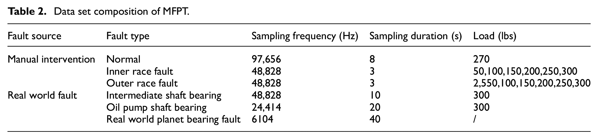
To analyze the MFPT datasets entirely, we treated the datasets in two categories: manual simulation faults including faults at different locations, under seven different loads, and three real-world bearing faults.

HFE enhancing

The signals are easily disturbed by external interference in the test rig, making the collected signals mixed with noise and causing the fault diagnosis difficult.

The signal denoising layer decomposes the signals into K modals. Although the parameter $α$ is adjusted by the test set, it will not affect the experimental results too much. Set penalty factor which is also bandwidth constraint $α$ = 2000 as a common value.^22,23 From equations (5)–(7), the expression of each modal and the iteration of the central frequency can be obtained. The K value is chosen through the instantaneous frequency. The signals are decomposed into K modals and the jth sampling point’s instantaneous frequency of the ith modal can be expressed as. $f_{ij}$ . Perform decomposition on the signals based each of K to obtain modal components ${\hat{u}}_{k} (ω)$ . And through inverse Fourier transform ${\hat{u}}_{k} (ω)$ can be transformed into time domain to get ${\hat{u}}_{k} (t)$ .

{\hat{u}}_{k} (t) = \frac{1}{2 π} \int_{- \infty}^{\infty} {\hat{u}}_{k} (ω) e^{j ω t}

(22)

Then analytic signals can be obtained through the Hilbert transform.

{\hat{z}}_{k} (t) = {\hat{u}}_{k} (t) + j {\hat{y}}_{k} (t)

(23)

Where

{\hat{y}}_{k} (t) = {\hat{u}}_{k} (t) * h (t)

(24)

h (t) = 1 / π t

(25)

* is the convolution operation. The instantaneous frequency is obtained by deriving the instantaneous phase of ${\hat{z}}_{k} (t)$ from time.

Then the mean of instantaneous of $f_{ij}$ can be expressed as

f_{i} = \frac{1}{N} \sum_{j} f_{ij}

(26)

N is the number of instantaneous frequencies in one modal.

According to the instantaneous frequency mean value method, the variation curve of the instantaneous frequency of signal data with K value can be obtained. We choose the oil pump bearing to show the trend of K in Figure 3.

Figure 3.

Instantaneous frequency-K value diagram.

If the K value is too large, the number of decomposition is too large, and the instantaneous jump phenomenon is severe. And the sudden jump will raise the mean value which will cause bending.

From Figure 3, the high-frequency component of the transient frequency jump raises the transient frequency average of the modal component, so the transient frequency average curve is bent suddenly at K = 13, so for oil pump bearing, K is 13. Similarly, K for the intermediate bearing is 8, and K for planet bearing is 6.

The K value is determined as 13, then the decomposition is performed by K to obtain the different modals. Different modals are shown in Figure 4.

Figure 4.

K modals of oil pump bearing.

From Figure 4, the first modal contains the most noise. Therefore the first modal is removed to eliminate high-frequency noise. Then the rest of the modal components are summed up to reconstruct the signals. The feature extraction layer adds a Gaussian window function instead of a wavelet basis function to the Fourier transform to obtain frequency information and amplitude information of signals. Then a complex matrix is obtained. To extract the features, the modular matrix is obtained by modular operation, and the time-frequency (TF) contour of two-dimensional images is obtained in Figure 5. From the TF curve in Figure 5, it is clear that the energy accumulation range of different fault radius frequencies is different.

Figure 5.

Time-frequency contour.

To better extract the features of bearing data with different fault categories, a total of 11 features are chosen according to the modulus matrix: skewness, kurtosis, peak to peak value, maximum frequency, the standard deviation of frequency, root mean square, maximum value, minimum value, average value, the average of absolute value and variance.

Although 11 features are extracted, the weights of the 11 features are different for fault signals. Dimensionality reduction of features is conducive to selecting the most important and independent features, and deleting redundant features reduces the amount of computation. Therefore, the signals are downscaled to generate new features to reduce computation.

Through formula (14), the contribution rate can be obtained, and the result is shown in Figure 6. From Figure 6, it can be seen that the first three characteristics account for the majority, and the total contribution of the first three features is 94.9342%. So 95% contribution rate is chosen as the selection criterion which leads to three eigenvectors for generating new features.

Figure 6.

Characteristics contribution.

For the bearing without fault, the new features are:

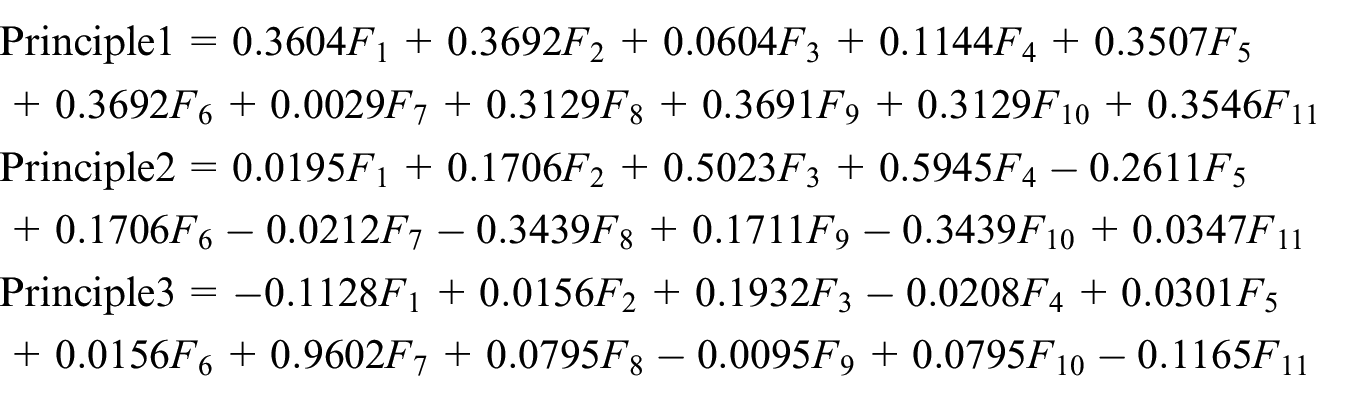
\begin{matrix} Principle 1 = 0.3604 F_{1} + 0.3692 F_{2} + 0.0604 F_{3} + 0.1144 F_{4} + 0.3507 F_{5} \\ + 0.3692 F_{6} + 0.0029 F_{7} + 0.3129 F_{8} + 0.3691 F_{9} + 0.3129 F_{10} + 0.3546 F_{11} \\ Principle 2 = 0.0195 F_{1} + 0.1706 F_{2} + 0.5023 F_{3} + 0.5945 F_{4} - 0.2611 F_{5} \\ + 0.1706 F_{6} - 0.0212 F_{7} - 0.3439 F_{8} + 0.1711 F_{9} - 0.3439 F_{10} + 0.0347 F_{11} \\ Principle 3 = - 0.1128 F_{1} + 0.0156 F_{2} + 0.1932 F_{3} - 0.0208 F_{4} + 0.0301 F_{5} \\ + 0.0156 F_{6} + 0.9602 F_{7} + 0.0795 F_{8} - 0.0095 F_{9} + 0.0795 F_{10} - 0.1165 F_{11} \end{matrix}

For the intermediate bearing fault, the new features are:

\begin{matrix} Principle 1 = 0.3584 F_{1} + 0.3603 F_{2} + 0.0511 F_{3} + 0.1464 F_{4} + 0.3538 F_{5} \\ + 0.3603 F_{6} + 0.0294 F_{7} + 0.3236 F_{8} + 0.3603 F_{9} + 0.3236 F_{10} + 0.3501 F_{11} \\ Principle 2 = 0.0235 F_{1} + 0.0977 F_{2} + 0.6438 F_{3} + 0.6092 F_{4} - 0.1617 F_{5} \\ + 0.0977 F_{6} + 0.0129 F_{7} - 0.2818 F_{8} + 0.0976 F_{9} - 0.2818 F_{10} + 0.0090 F_{11} \\ Principle 3 = - 0.0180 F_{1} - 0.0158 F_{2} - 0.0132 F_{3} + 0.0065 F_{4} - 0.0047 F_{5} \\ - 0.0158 F_{6} + 0.9990 F_{7} + 0.0050 F_{8} - 0.0271 F_{9} + 0.0050 F_{10} - 0.0104 F_{11} \end{matrix}

For the oil pump bearing fault, the new features are:

\begin{matrix} Principle 1 = 0.3625 F_{1} + 0.3539 F_{2} - 0.0538 F_{3} + 0.0288 F_{4} + 0.3657 F_{5} \\ + 0.3539 F_{6} + 0.0487 F_{7} + 0.3374 F_{8} + 0.3537 F_{9} + 0.3374 F_{10} + 0.3541 F_{11} \\ Principle 2 = 0.0060 F_{1} + 0.2479 F_{2} + 0.5220 F_{3} + 0.5980 F_{4} - 0.2034 F_{5} \\ + 0.2479 F_{6} - 0.0273 F_{7} - 0.2676 F_{8} + 0.2484 F_{9} - 0.2676 F_{10} + 0.0046 F_{11} \\ Principle 3 = - 0.0542 F_{1} - 0.0048 F_{2} + 0.0622 F_{3} + 0.0111 F_{4} - 0.0061 F_{5} \\ - 0.0048 F_{6} + 0.9940 F_{7} + 0.0124 F_{8} - 0.0145 F_{9} + 0.0124 F_{10} - 0.0659 F_{11} \end{matrix}

For the planet bearing fault, the new features are:

\begin{matrix} Principle 1 = 0.3587 F_{1} + 0.3599 F_{2} + 0.0282 F_{3} + 0.1287 F_{4} + 0.3657 F_{5} \\ + 0.3539 F_{6} + 0.0487 F_{7} + 0.3374 F_{8} + 0.3537 F_{9} + 0.3374 F_{10} + 0.3541 F_{11} \\ Principle 2 = 0.0282 F_{1} + 0.1034 F_{2} + 0.6445 F_{3} + 0.6209 F_{4} - 0.1493 F_{5} \\ + 0.1034 F_{6} - 0.0429 F_{7} - 0.2662 F_{8} + 0.1036 F_{9} - 0.2662 F_{10} + 0.0174 F_{11} \\ Principle 3 = 0.0035 F_{1} + 0.0182 F_{2} + 0.0319 F_{3} + 0.0462 F_{4} + 0.0116 F_{5} \\ + 0.0182 F_{6} + 0.9976 F_{7} + 0.0181 F_{8} + 0.0105 F_{9} + 0.0181 F_{10} - 0.0024 F_{11} \end{matrix}

Then new features are spliced together to form new features. Converting the one-dimensional signals into two-dimensional space helps to further analyze the characteristics of faults and thus classify different faults. After regenerating new features from the matrix, the new one-dimensional vector is reconstructed. After that, the signals are dynamically transformed into polar coordinates to form two-dimensional feature pictures. Since all the values are in the same scale of [−1,1], every pixel in the picture can be expressed as different colors corresponding to values according to equation (17).

Fault classification

The labels of MFPT dataset corresponding to seven different loads are 0, 1, 2, 3, 4, 5, and 6 respectively. Labels corresponding dissimilar real-world faults are 0, 1, 2, and 3 respectively. The bearing data under seven different loads are first used for training.

The CNN structure is designed concerning the VGG structure, and a simplification is made based on it²⁴ after the HFE method to diagnose faults. The structure is shown in Figure 7. Since the CNN structure is used to further extract deeper features and classify the different fault features enhanced by HFE. The results of the analysis are mainly to compare the impact of the adoption of HFE on the classification results of CNN, so the CNN structure is not the main. Simplified analysis based on VGG structure can not only achieve the purpose of comparison but also improve the calculation speed.

Figure 7.

Schematic diagram of the CNN structure.

The picture size is set to 128 × 128 pixels. Therefore, training picture datasets are formed in each fault state. The fault classification problem for different loads of the MFPT dataset is a seven classification problem for the loads that have seven different states. The three real-world faults plus the data without faults can be counted as a four-category discriminant. For different defects, characteristic values are different, the defect characteristic diagrams are also not the same. The CNN structure is used to learn the features on a deeper level. The network structure is simplified to reduce the computation and speed up the training.

A total of nine convolution layers and three Max-pooling layers are connected to learn the characteristic maps. Since the pictures that contain faults are hard to classify, it needs several convolution layers to learn the features. And the max-pooling layers are after the convolution layers to further obtain the optimal features.

To classify the different types of faults, the features are flattened, and fully-connected layers integrate the feature representation in the next to output the result as a value. Then dropout is chosen to avoid over-fitting. An activation function of ReLU is selected in every convolution layer and fully-connected layer. Choose epoch of 1500 and batch size of 100 for the model to train. The proportion of the test set is set to 33%, dropout is 0.25 and the weight decay is 1e⁻⁵, then the prediction discrimination confusion matrix is obtained in Figure 8 which is trained by MFPT datasets. Inner race and outer race bearing under seven dissimilar loads results and three real-world bearing faults with normal bearing results are shown in Figure 8.

Figure 8.

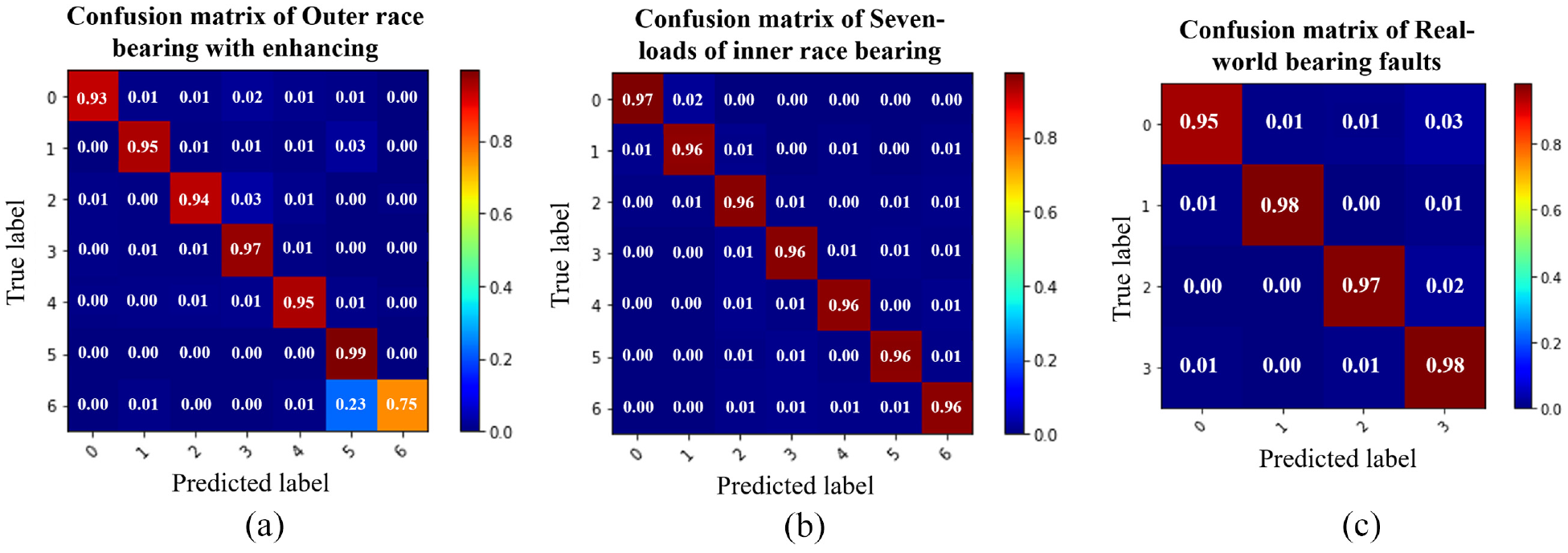
The confusion matrix of the MFPT data set.

From the confusion matrix of MFPT in Figure 8, we can get when the epoch is set to 1500 and the batch size is 100, the model, used to distinguish the seven different loads of inner and outer race bearing faults has dissimilar accuracy when recognizing faults. Not all the accuracies are high. But the model used to distinguish three real-world bearing faults with one normal bearing is performing well. The reason for the difference in recognition accuracy of different models is related to the parameters of model training.

In order to evaluate the training effect of the model, the evaluation index of learning is selected as: precision, recall, f1 and loss.

When it is a four-categories classification problem, the correct classification and prediction results can be expressed in Table 3, the accurate classification samples are distributed on the diagonal.

Table 3.

Label and prediction result representation.

Label prediction	A	B	C	D
A	AA	AB	AC	AD
B	BA	BB	BC	BD
C	CA	CB	CC	CD
D	DA	DB	DC	DD

Generally, n classes are calculated as N binary tasks, and each class is processed and filled in separately. For A, the calculating progress is shown in Table 4.

Table 4.

Label and prediction result representation of A.

Label prediction	Label = A	Label = non A
Prediction = A	TP(A) = AA	FP(A) = AB + AC + AD
Prediction = non A	FN(A) = BA + CA + DA	TN(A) = BB + BC + BD
		CB + CC + CD
		DB + DC + DD

From Table 4 we can calculate the prediction of A which is:

\bar{P} = \frac{TP}{TP + FP} = \frac{AA}{AA + (AB + AC + AD)}

(27)

Then we can also calculate following the same progress to get $\bar{P}$ .

\bar{P} = \frac{P_{A} + P_{B} + P_{C} + P_{D}}{4}

(28)

The value of recall is:

\bar{R} = \frac{TP}{TP + FN} = \frac{AA}{AA + (BA + CA + DA)}

(29)

Then we can also calculate the same progress to get $\bar{R}$ .

\bar{R} = \frac{R_{A} + R_{B} + R_{C} + R_{D}}{4}

(30)

The value of $F_{A}$ :

F_{A} = \frac{2 P_{A} R_{A}}{P_{A} + R_{A}}

(31)

Then $\bar{F}$ can be obtained.

\bar{F} = \frac{F_{A} + F_{B} + F_{C} + F_{D}}{4}

(32)

Loss:

CE (x) = - \sum_{i = 1}^{C} y_{i} \log f_{i} (x)

(33)

Where x is the input sample, C is the total number of categories to be classified, $y_{i}$ is the real label of the ith category and $f_{i} (x)$ is the output values for corresponding models.

For batch, the loss of all samples in the batch is averaged.

CE (x)_{final} = \frac{\sum_{b = 1}^{N} CE (x^{(b)})}{N}

(34)

The calculation of precision, recall, f1, and loss is illustrated by the four classification tasks.

After training, four metric values can be obtained about the model under seven different loads in the MFPT data sets. For the outer race bearing, the four indexes are precision: 0.9787, loss: 0.0690, f1: 0.977, and recall: 0.975. For the inner race bearing the indexes are: precision: 0.9780, loss: 0.0733, f1: 0.9754, recall: 0.9729. For real-world bearing failures the indexes are precision: 0.9921, loss: 0.0266, f1: 0.9920, recall: 0.9918.

Ablation experiments and analysis

Some parameters will affect the training accuracy of the model, such as the batch size of the training set. To further improve the fault classification accuracy of the model, the batch size is adjusted. We use four learning evaluation indexes (precision, recall, f1, and loss) that are mentioned above to compare the model training ability under different batch sizes. The obtained training results for different loads on the inner and outer race bearing of the MFPT datasets are shown in Table 5.

Table 5.

Effects of batch size parameter on experiment results.

	Index	Batch size = 64	Batch size = 100
Outer	Precision & Loss
	F1 & Recall
	Accuracy	99.63%	97.79%
Inner	Precision & Loss
	F1 & Recall
	Accuracy	99.42%	97.41%

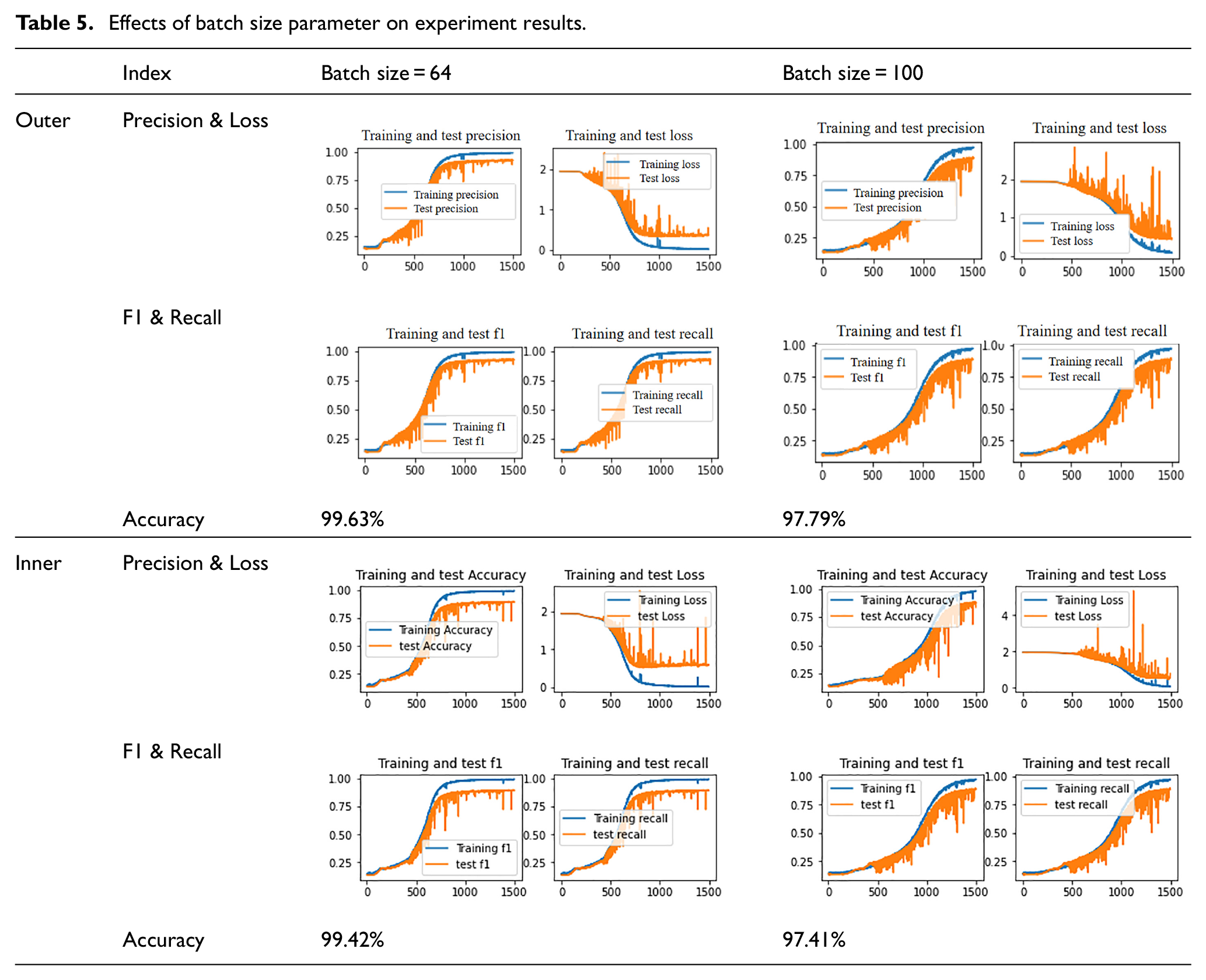
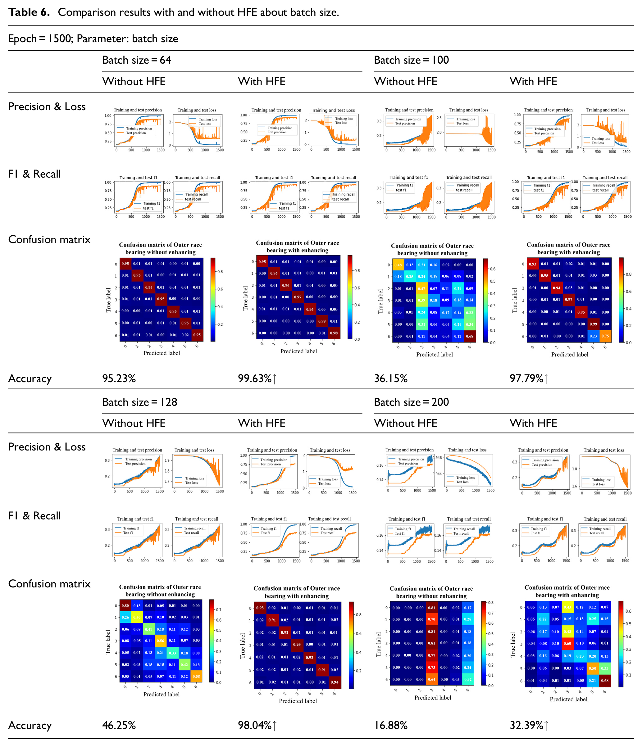
It can be seen from Table 5 that when the batch size is 64, the results have converged basically when the epoch equals 1000. In order to further illustrate the effectiveness of the HFE method, the CNN model is directly used in this paper to process the raw signals for classification. Although fault diagnosis is no longer satisfied with the use of traditional classification methods, the traditional methods still occupy certain advantages in the pre-processing of vibration data. Various neural network models can to learn the features by themselves. Nevertheless, the bearing fault signals collected by the sensors do not have obvious characteristics and are prone to produce mixed features. In this case, the application of the CNN model used alone for training is poor and the results can be seen from the comparison in Tables 6 and 7. Take ablation experiments on the MFPT datasets. Bearings with different loads on the outer race are shown as an example to compare the impact of HFE on model training when the batch size and epoch are changed. Batch sizes equal 64 and equal 128 are often used in network training. Since when batch size equals 64 the model has achieved good results, we took two more batch sizes which are 100 and 200 as parameters in experiments to illustrate the classification effect of the CNN model before and after signal enhanced by HFE. Since a good fault diagnosis accuracy has been achieved when epoch equals 1000 in Table 5, two groups of epoch values are taken up and down respectively for experiments based on this epoch value. At the same time, in order to illustrate the extreme situation, another group of epochs equal 100 is taken for experiments to see the effect of HFE on feature enhancement and the help of CNN classification in the case of training underfitting. From Tables 6 and 7, we can get the conclusion that the HFE can improve the accuracy of the model to some extent even though the parameters of the CNN can have an impact on the training results.

Table 6.

Comparison results with and without HFE about batch size.

Epoch = 1500; Parameter: batch size
	Batch size = 64		Batch size = 100
	Without HFE	With HFE	Without HFE	With HFE
Precision & Loss
F1 & Recall
Confusion matrix
Accuracy	95.23%	99.63%↑	36.15%	97.79%↑
	Batch size = 128		Batch size = 200
	Without HFE	With HFE	Without HFE	With HFE
Precision & Loss
F1 & Recall
Confusion matrix
Accuracy	46.25%	98.04%↑	16.88%	32.39%↑

Table 7.

Comparison results with and without HFE about epoch.

Batch size = 64; Parameter: epoch
	Epoch = 100		Epoch = 500
	Without HFE	With HFE	Without HFE	With HFE
Precision & Loss
F1 & Recall
Confusion matrix
Accuracy	14.78%	18.38%↑	28.85%	59.87%↑
	Epoch = 1000		Epoch = 1500
	Without HFE	With HFE	Without HFE	With HFE
Precision & Loss
F1 & Recall
Confusion matrix
Accuracy	83.65%	97.67%↑	95.23%	99.63%↑

In Table 6, it can be seen that the accuracy increases significantly when batch size equals 100, from 36.15% to 97.79%. And even when batch size equals 200 which causes a low accuracy, the HFE method can also improve the classification accuracy from 16.88% to 32.39%. In Table 7, the batch size is fixed at 64, and experiments are conducted with epoch changing. The HFE method also has a good effect on the results. When the epoch equals 1500, the accuracy is up to 99.63%. In these two tables, the training accuracy of the model is greatly reduced when the batch size is too big or the epoch is too small. However, even in this case, the accuracy can still be improved greatly by applying the HFE method. In hence, the HFE method can greatly enhance the characteristics of faults and improve the accuracy of fault diagnosis. To more intuitively display the feature enhancement effect of HFE on the signals in different noise environments, we intercepted a section of the signal and added different Gaussian noises, which are −5, −10, 5, and 10 dBW respectively. The results are shown in Figure 9. It can be seen from Figure 9 that the region with the largest time-domain signal oscillation on the left in Figure 9(a) forms the feature formed by line crossing in the middle feature map, and the line crossing feature is enhanced after feature enhancement by HFE. By adding different Gaussian noise to the original signal, the time-domain signal in Figure 9(b)–(e) can be formed. The features after adding noise become unclear which is hard to diagnose, but the features become obvious after processing through HFE. Therefore, HFE can enhance the fault features even in high noise scenarios.

Figure 9.

Feature images in different noise after HFE: (a) original signals; (b)signals with 5 dBW noise; (c) signals with 10 dBW noise; (d) signals with −5 dBW noise; and (e) signals with −10 dBW noise.

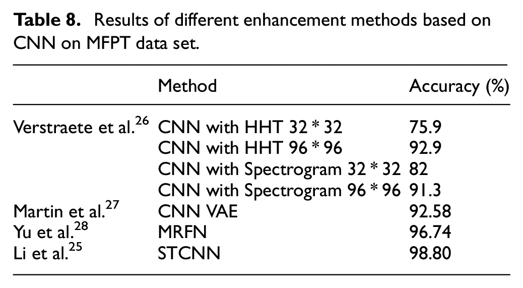
With the development of neural network methods, more and more scholars use CNN for fault diagnosis and classification. The comparative results of CNN with different enhancement methods are shown in Table 8. It can be seen that many scholars have achieved good results in classification for MFPT datasets whose accuracy of fault classification is up to 98.80% according to STCNN proposed by Li et al.²⁵ Our classification also achieves good results which are higher than 99%. However, the HFE method proposed by us only combines with a simple CNN structure for analysis. Therefore, the HFE method proposed by us can greatly enhance the fault features and improve the accuracy of the classification model.

Table 8.

Results of different enhancement methods based on CNN on MFPT data set.

	Method	Accuracy (%)
Verstraete et al.²⁶	CNN with HHT 32 * 32	75.9
	CNN with HHT 96 * 96	92.9
	CNN with Spectrogram 32 * 32	82
	CNN with Spectrogram 96 * 96	91.3
Martin et al.²⁷	CNN VAE	92.58
Yu et al.²⁸	MRFN	96.74
Li et al.²⁵	STCNN	98.80

Conclusion and future work

Signals are easily drowned in high noise which makes features hard to extract and train. Based on this, the HFE method is proposed for the CNN-based fault diagnosis. HFE contains three layers including a signal denoising layer, feature extraction layer, and feature transforming layer. Through HFE, the weak fault features buried in high noise are enhanced and can prevent noise interference. Then CNN is used to mine deeper features and diagnose the faults.

To verify the effectiveness of the proposed HFE method, datasets of bearings are chosen as an example since bearing signals are easily affected by the noise. Through training, the model can efficiently distinguish faults under different conditions including bearing faults under different loads and locations, artificial faults, and real faults. The accuracies of the MFPT datasets are great which are all above 99% in different conditions. At the same time, signals in different noise scenarios were simulated and transformed into two-dimensional images to intuitively show features that fully illustrate the robustness of the model.

Although the model used in this paper achieves good results, the CNN used has been simplified without considering the specific design of the model in depth. Therefore, the structure of the model needs to be further considered in the future, maybe using some relevant optimization algorithms. With that, the proposed HFE can be combined with a more optimized network model for fault classification and diagnosis.

Footnotes

Handling Editor: Chenhui Liang

Declaration of conflicting interests

The author(s) declared no potential conflicts of interest with respect to the research, authorship, and/or publication of this article.

Funding

The author(s) disclosed receipt of the following financial support for the research, authorship, and/or publication of this article: This work has been funded by the National Natural Science Foundation of China (51905476), the Public Welfare Technology Application Projects of Zhejiang Province, China (LGG22E050008), the Jiangsu Province Science and Technology Achievement Transforming Fund Project (BA2018083).

ORCID iDs

Zili Wang

Lemiao Qiu

References

Liu

Jia

, et al. Tool wear estimation using a CNN-transformer model with semi-supervised learning. Meas Sci Technol 2021; 32: 125010.

Zhong

, et al. Diagnosis intermittent fault of bearing based on EEMD-HMM. In: International conference on mechatronics and intelligent robotics, 2018, pp.174–182. Cham: Springer.

Jiang

Yin

Kaynak

Data-driven monitoring and safety control of industrial cyber-physical systems: basics and beyond. IEEE Access 2018; 6: 47374–47384.

Tamilselvan

Wang

Failure diagnosis using deep belief learning based health state classification. Reliab Eng Syst Saf 2013; 115: 124–135.

Cao

Ding

Jia

, et al. A novel temporal convolutional network with residual self-attention mechanism for remaining useful life prediction of rolling bearings. Reliab Eng Syst Saf 2021; 215: 107813.

Lyu

Huo

Cheng

, et al. Distributed optical fiber sensing intrusion pattern recognition based on GAF and CNN. J Lightwave Technol 2020; 38: 4174–4182.

Zhang

Peng

, et al. A new deep learning model for fault diagnosis with good anti-noise and domain adaptation ability on raw vibration signals. Sensors 2017; 17: 425.

Mao

Lin

, et al. Recognition of rolling bearing running state based on genetic algorithm and convolutional neural network. Adv Mech Eng 2022; 14: 168781402110729.

Tang

Liao

Chen

, et al. A novel convolutional neural network for low-speed structural fault diagnosis under different operating condition and its understanding via visualization. IEEE Trans Instrum Meas 2021; 70: 1–11.

10.

Wang

Compound mechanical fault diagnosis based on CMDE. Adv Mech Eng 2022; 14: 168781322210805.

11.

Wang

Liu

Liao

, et al. An enhanced diagnosis method for weak fault features of bearing acoustic emission signal based on compressed sensing. Math Biosci Eng 2021; 18: 1670–1688.

12.

Medina

Macancela

Lucero

, et al. A LSTM neural network approach using vibration signals for classifying faults in a gearbox. In: International conference on sensing, diagnostics, prognostics, and control (SDPC), Beijing, China, 15–17 August 2019, pp.208–214. New York, NY: IEEE.

13.

Sawalhi

Randall

Endo

The enhancement of fault detection and diagnosis in rolling element bearings using minimum entropy deconvolution combined with spectral kurtosis. Mech Syst Signal Process 2007; 21: 2616–2633.

14.

Cai

, et al. An enhanced multipoint optimal minimum entropy deconvolution approach for bearing fault detection of spur gearbox. J Mech Sci Technol 2019; 33: 2573–2586.

15.

Srimani

Ghosh

Rahaman

Wavelet transform based fault diagnosis in analog circuits with SVM classifier. In: IEEE international test conference India, Bangalore, India, 12–14 July 2020, pp.1–10. New York, NY: IEEE.

16.

Yang

Huang

, et al. Rotating machinery fault diagnosis using long-short-term memory recurrent neural network. IFAC-PapersOnLine 2018; 51: 228–232.

17.

Zhu

Song

Yang

, et al. A bearing fault diagnosis method based on L1 regularization transfer learning and LSTM deep learning. In: IEEE international conference on information communication and software engineering (ICICSE), Chengdu, China, 19–21 March 2021, pp.308–312. New York, NY: IEEE.

18.

Dragomiretskiy

Zosso

Variational mode decomposition. IEEE Trans Signal Process 2014; 62: 531–544.

19.

Xia

Wang

Song

, et al. Fault diagnosis of flexible production line machining center based on PCA and ABC-LVQ. Proc IMechE, Part B: J Engineering Manufacture 2021; 235: 594–604.

20.

Wang

Oates

. Imaging time-series to improve classification and imputation. arXiv:1506.00327, 2015.

21.

Machinery fault prevention technology bearing data, https://mfpt.org/fault-data-sets/ (2012).

22.

Deng

Zhang

Zhao

Intelligent identification of incipient rolling bearing faults based on VMD and PCA-SVM. Adv Mech Eng 2022; 14: 168781402110729.

23.

Gai

Shen

, et al. An integrated method based on hybrid grey wolf optimizer improved variational mode decomposition and deep neural network for fault diagnosis of rolling bearing. Measurement 2020; 162: 107901.

24.

Simonyan

Zisserman

Very deep convolutional networks for large-scale image recognition. Comput Sci 2014.

25.

Deng

, et al. Sensor data-driven bearing fault diagnosis based on deep convolutional neural networks and S-transform. Sensors 2019; 19: 2750.

26.

Verstraete

Ferrada

Droguett

, et al. Deep learning enabled fault diagnosis using time-frequency image analysis of rolling element bearings. Shock Vib 2017; 2017: 1–17.

27.

San Martin

López Droguett

Meruane

, et al. Deep variational auto-encoders: A promising tool for dimensionality reduction and ball bearing elements fault diagnosis. Struct Health Monit 2019; 18: 1092–1128.

28.

Wang

Multiscale representations fusion with joint multiple reconstructions autoencoder for intelligent fault diagnosis. IEEE Signal Process Lett 2018; 25: 1880–1884.

Signals hierarchical feature enhancement method for CNN-based fault diagnosis

Abstract

Keywords

Introduction

Method

Hierarchical feature enhancement method

Signal denoising layer

Feature extraction layer

Feature transformation layer

Fault classification method

Experiment

MFPT data set

HFE enhancing

Fault classification

Ablation experiments and analysis

Conclusion and future work

Footnotes

Declaration of conflicting interests

Funding

ORCID iDs

References