Sage Journals: Discover world-class research

Abstract

With the development of the manufacturing industry and information technology, the quality requirements of products are getting higher and higher. A cutting tool is one of the important factors affecting product quality, so it is of great significance to study cutting tool wear. In this paper, the influence of Ni-Cr alloy on milling cutter wear was studied. Deep learning is widely used in the neighborhood of signal recognition. In this paper, a convolution neural network with residual structure is proposed to classify the wear state of cutting tools. The input of the model is the collected vibration signal, and the output is the classification of tool wear. A convolution neural network can automatically extract the characteristics of signals and identify different types of wear signals. The experimental results show that the convolution neural network with residual structure can converge faster and have higher accuracy than the traditional convolution neural network and the accuracy of tool wear classification is about 98.5%. The loss rate of the model is only about 0.25%.

Keywords

Convolution neural network residual structure tool wear monitoring

Introduction

With the rise of the manufacturing industry, intelligent manufacturing is also developing. China has also joined the trend of world development, which means that China’s manufacturing industry is also developing in a smarter direction. Traditional production workshop is gradually replaced by intelligent production workshop, and the quality of products is getting higher and higher. In the production process, the degree of tool wear has a great influence on the quality of the workpiece. Therefore, Tool Condition Monitoring (TCM) is of great significance to improve machining efficiency and reduce cost loss.¹ There are two methods of tool wear measurement: direct measurement and indirect measurement. Direct measurement includes optical instrument measurement, machine vision measurement, radiographic measurement, etc; These measurement methods are affected by the processing environment. There is no way to directly measure the tool wear value online in production and processing, and it is rarely used in actual processing. Therefore, indirect measurement methods are widely used, using sensors to collect cutting force.² Guo et al.³ compared different monitoring signals, it is proposed that deep learning can improve the prediction accuracy. Zhu et al.⁴ proposed a long-term and short-term memory neural network. Compared with different neural networks, the results show that the proposed network has high accuracy. vibration.⁵ Cao et al.⁶ aimed at the bearing fault problem, an improved convolutional neural network is proposed, and the results show that the proposed method has good stability. Li et al.⁷ proposed a deep long-short memory network to predict the tool wear state. Zhao et al.⁸ proposed bidirectional BiLSTM to identify different fault signals, and acoustic emission signals.⁹ Wu et al.¹⁰ proposed a convolution automatic encoder to train the model, and the results show that the error of the proposed model is very small. Fatemeh et al.¹¹ proposed convolution neural network to process the data by wavelet, and the results show that the proposed method has higher accuracy. To analyze the time domain signals. BP neural network (BPNN),¹² Hidden Markov Model (HMM),¹³ Bayesian network, Support Vector Machine (SVM),¹⁴ and other machine learning models are used for prediction. Before using this machine learning network model, it is necessary to preprocess the data, extract the features contained in the data, and select the features with a large correlation coefficient with wear as the input of the model through the Pearson correlation coefficient criterion. The method often relies on the experience of the operator, and the whole process takes a lot of time, while the deep learning (DL) method can avoid the above problems.

In recent years, deep learning has continued to develop, and convolutional neural networks have been widely used, mainly in the fields of image recognition and speech recognition.¹⁵ In the industrial field, neural networks have also been used in certain applications, such as tool life prediction, fault diagnosis, tool wear detection, etc. Lin et al.¹⁶ used a deep neural network to classify tool wear. Cao et al.¹⁷ mined hidden features in data by changing the structure of a convolutional neural network and adding dense connection blocks. The results proved that a convolutional neural network had a smaller loss function value and higher accuracy than other machine learning networks. Zhang et al.¹⁸ proposed to convert the one-dimensional data signal into a two-dimensional spectrogram and input it into a convolutional neural network, proving that the loss function and accuracy of Wearnet are better than other deep learning networks. He et al.¹⁹ adopted the method of combining the convolutional neural network and the long-term memory network and changed the number of neurons in the convolutional neural network. By comparison, the accuracy rate was higher when the number of neurons was 64. Chen et al.²⁰ proposed an improved convolutional neural network and added the Attention mechanism. Compared with the deep learning network models used in other literature, the training speed is faster and the accuracy rate is higher. Liu et al.²¹ used an improved convolutional neural network model (CNN) and a bidirectional long-short-term memory model (BiLSTM) to monitor tool wear through wavelet threshold noise reduction preprocessing. Compared with the traditional neural network model, this model is able to perform better; Tao et al.²² used Fourier transform to process the data and introduced the AdaBoost algorithm into the regression tree to improve the performance of the model. The results showed that the accuracy and stability of the improved model are significantly promoted; Qin et al.²³ used the method of model combination and genetic algorithm to optimize cutting parameters and obtained the relationship between cutting parameters and tool wear. The results showed that the wear after cutting parameters optimized by a genetic algorithm was smaller. Xie et al.²⁴ used power sensors to collect data and principal component analysis (PCA) to extract features. Finally, a C-SVM model was established for verification and compared with BP neural network, the results showed that the accuracy of the C-SVM model was higher than that of the BP neural network; Li et al.²⁵ proposed an improved artificial neural network to predict tool wear and cutting force. The experimental results showed that the neural network prediction results had smaller errors than the empirical formula; Tamilselvan and Wang²⁶ used the data collected by the sensor to realize the fault diagnosis of the transformer. Benkedjouh et al.²⁷ used principal component analysis to reduce data dimension, and SVM to predict wear.

In the above methods, it is often time-consuming and laborious for machine learning models to extract features based on the experience of researchers; Most of the deep learning models adopt two-dimensional convolutional neural networks, which need to convert data into a spectrogram, which will cause data information loss. The data collected by the sensor is time-series data, which has multidimensional and time series characteristics. Therefore, to ensure the integrity of the data information, this paper proposes a one-dimensional convolution neural network with a residual structure to extract the features of the data and identify the wear classification corresponding to the feature signals. Adam optimization model is adopted in the model so that the model can quickly converge to obtain the minimum loss function. Add a Dropout layer to the fully connected layer to randomly ignore certain neurons to prevent the model from overfitting. The research shows that the deep learning network model proposed in this paper has high accuracy and can satisfy the classification of tool wear.

Tool wear monitoring framework

The tool wear monitoring framework is shown in Figure 1. During the experiment, CNC machine tools are used for processing, and sensors are used to collect vibration signals, cutting force signals, and acoustic emission signals during processing. The vibration signals and cutting force signals include three dimensions of x, y, and z, plus sound send signals, collecting a total of seven-dimensional data. In the process of machining, there is no way to realize online measurement. The wear amount of the flank face is observed and recorded through a microscope every time the tool travels a stroke until the tool reaches the level of sharp wear and cannot be processed again. The convolutional neural network does not determine the weight of each layer of the network in the early stage of training. The data set is divided into a training set and a validation set. The training set is used to train the weight of the network model. After training, the mapping relationship between input and output is obtained. After determining the initial weights, the validation set input is used to evaluate the performance of the model. When the performance of the model output in the two data sets is almost the same, it indicates that the model has not been over-fitted, and the model training is completed.

Figure 1.

Tool wear monitoring frame.

The establishment of one-dimensional convolutional network model

The tool wear monitoring adopts a one-dimensional convolutional neural network. The network model includes a convolutional layer (CONV), a batch normalization layer (BN), a pooling layer (POOL), and a fully connected layer. The convolutional layer extracts and analyzes the data through a sliding window to change the data dimension; the pooling layer is mainly used to select the optimal features, reduce the amount of computation, and improve the generalization ability of the model. The whole connection layer spreads the pooled 2D features to the 1D data features and classifies them from the input layer to the output layer through continuous iteration and training.

Convolutional layer

The convolution layer is responsible for feature extraction of data, randomly selecting a piece of data to learn some features, using the learned features as a filter, and then scanning the features of other data. Every position of the data has a corresponding feature value, and this process of continuous feature learning is called convolution. The size, step size, and some convolution kernels will all affect the accuracy of the model. The calculation formula of convolution is shown in formula (1), The convolution process is shown in Figure 2.

Z^{l + 1} = \sum_{c = 1}^{C} (w_{c}^{l + 1} Z^{l}) + b

(1)

Figure 2.

Convolution process.

Among them, w is the weight of the convolution kernel, c is the number of channels in this layer, Zl is the output feature matrix of the previous layer, and b is the bias constant. The calculation method of the convolution layer is the inner product, and the convolution kernel is multiplied by the selected data area and then added.

Pooling layer

The pooling layer is generally located after the convolutional layer, which further extracts the features of the convolutional layer and reduces the data dimension. Pooling operations include average pooling and max pooling. Average pooling is the average of the selections; max pooling is the selection of the largest value of the pooled area. The max-pooling operation is shown in Figure 3.

Figure 3.

Maximum pooling process.

The full connection layer

The role of the full connection layer is to classify, which is generally located at the last layer of the network model. The full connection layer can flatten the features extracted from the convolution layer and pool layer. In the full connection layer, the activation function softmax is often used for classification. The classification process of the full connection layer is shown in Figure 4.

Figure 4.

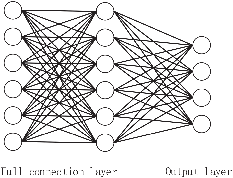
Full connection layer.

Residual structure

With the deepening of the network, the performance of the network will decline, which will lead to a low training accuracy, and the phenomenon of gradient disappearance may also occur. Studies have shown that residual connections can effectively prevent these phenomena from occurring. The structure of the residual module is shown in Figure 5.²⁸

Figure 5.

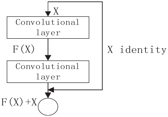
Residual block structure.

The polyline connection in the figure is a near-channel connection. This connection method can skip a part of the convolutional layer to speed up the convergence of the model, and can also directly transmit important information to the next layer of the network. The output of the residual is shown in formula (2).

G (x_{l + 1}) = F (x_{l}) + x_{l}

(2)

Among them, x_l is the input of the previous layer, and F(x_l) is the output after the convolutional layer.

1D convolutional neural network batch normalization and regularization

Batch Normalization (BN) is used before the activation function to obey the normal distribution of the variance and mean of the output, reduce the dependence of neurons, improve the performance of the model, and accelerate the convergence of the network. During the model training process, due to the number of samples, and the complexity of the model, the training results are prone to overfitting. In order to get a better model, a dropout layer needs to be added to the fully connected layer, which can randomly shield some neurons in the network, each layer is equivalent to a new network, and the correlation between layers is reduced, allowing the model adapt to the new network environment and increase the robustness of the model. During the forward propagation of the network, the masked neurons have no effect, and the dropout layer is turned off when the model is trained on the validation set so that all neurons can have an effect on the model.

Residual structured convolutional network model

The structure of adding residual blocks to a one-dimensional convolutional neural network is shown in Figure 6. In the figure, two residual blocks are connected in series, and each residual block includes two convolution layers and two BN layers.

Figure 6.

Residual network structure.

The input of the previous layer will be divided into two parts, one part is stored in the near-channel connection (X identity), and the other part is passed through the convolutional layer and the BN layer, and the output result and the stored near-channel connection are added as the output of the residual block. In this paper, two residual blocks are connected to operate on the data set, and finally, the classification is carried out through the softmax layer. The activation function relu is added to the neural network of each layer. The purpose of adding the activation function is to increase the nonlinear ability of the model. The summary of the network model is shown in Table 1, and finally, the wear classification results are output. Since the dimensions of the collected data are different, in order to eliminate the dimension, the data must be standardized, and the standardized treatment is shown in formula (3).

x_{k} = \frac{x - x_{min}}{x_{max} - x_{min}}

(3)

Table 1.

Network summary.

Network layer	Number	Size	Stride	Activation function
Convolutional layer	64	7 × 1	2	Relu
BN layer	–	–	–	–
Pooling layer	64	3 × 1	2	–
Convolutional layer	64	1 × 1	1	Relu
BN layer	–	–	–	–
Convolutional layer	64	3 × 1	1	Relu
BN layer	–	–	–	–
Convolutional layer	64	1 × 1	1	Relu
Convolutional layer	64	1 × 1	1	Relu
BN layer	–	–	–	–
BN layer	–	–	–	–
Add	–	–	–	–
Pooling layer	64	4 × 1	4	–
Flatten	–	–	–	–
Dense1	-	–	–	Relu
Dense2	-	–	–	Softmax

Among them, x_min is the minimum value of the data, and x_max represents the maximum value of the data so that the data range can be controlled between [0,1]. The error between the true value and the predicted value is calculated using Adam for the optimization algorithm, and the loss function is defined as shown in equation (4).²⁰

M S E = \sum_{i = 1}^{n} \frac{1}{n} {(\overset{'}{y} - y)}^{2}

(4)

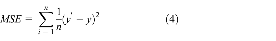
Among them, y′ is the predicted value, y is the real value, n is the number of data samples, and the mean square error between the predicted value and the real value is used as the loss function. The convolutional neural network needs to update the gradient during forwarding propagation, and adjust the weight of each layer of the network so that the predicted value can continuously approach the real value. The update of the gradient is shown in formula (5).¹⁹

W_{l + 1} = W_{l} - η \frac{\partial_{MSE}}{\partial_{W_{l}}}

(5)

Among them, W_l is the weight and is the learning rate. Continue to descend along the gradient direction, the faster the function value decreases, the smaller the loss function value.

Model training

After the model is established, the weight parameters of the model need to be iterated through the input data, and the iteration is stopped until the set conditions of the model are reached. The test set is used to verify the quality of the model weight. The model training process is shown in Figure 7.

Figure 7.

Training flow chart of model.

The input data is divided into two parts: the validation set and the training set. At the beginning of the model, there is only the initialized weight. This weight is randomly assigned and the accuracy is not high. The training set is used to train the weight of the model, and the weight is continuously adjusted until the loss function reaches convergence. The function reaches convergence; the purpose of adding the validation set is to test the performance of the trained weights in the new data set. If the performance is stable, it means that the weights of the model are appropriate.

Results

Experimental conditions

In order to verify the validity of the model, this paper uses the data of the tool wear open competition held by the American PHM Association in 2010.²⁹ The experimental equipment and cutting parameters are shown in Table 2.

Table 2.

Experimental equipment and parameters.

Machine	Roders Tech RFM760
Force sensor	Kistler 9265B
Vibration sensor	Kistler three-axis accelerometer
Acoustic emission sensor	Kistler Acoustic emission sensor
Charge amplifier	Kistler charge amplifier
Wear Gauge	LEICA MZ12
Data acquisition equipment	NI DAQ PCI 1200 capture card
cutter	Ball nose carbide milling cutter
Workpiece material	Inconel718 (HBS400)
Spindle speed (rpm)	10400
Feed rate (mm/min)	1555
Cutting width (mm)	0.125
depth of cut (mm)	0.2
Cutting method	Climb milling
Frequency	50kHz

During the experiment, the data of the machining process is collected by sensors, and the experimental device is shown in Figure 8. Three force sensors are installed at the bottom of the workpiece to measure the cutting forces in X, Y, and Z directions. Three acceleration sensors are connected to the spindle of the machine tool to collect the vibration signals in the machining process. The acoustic emission sensor connects the workpiece and collects the stress wave in the machining process.

Figure 8.

Schematic diagram of the experimental platform.

When the tool cuts 108 mm along the X-axis, use a microscope to check the wear amount of the tool flank. Each tool takes 315 strokes, record the three flank wear values corresponding to each stroke, and takes the maximum value. The wear curve is shown in Figure 9. The wear curve is divided into three categories: initial wear (0–32), mid-term wear (33–150), and sharp wear (151–315). Data is stored on the computer.

Figure 9.

Tool wear curve.

The x axis is the cutting stroke, and the y axis is the tool wear. It can be seen from the figure that the initial wear is fast but the amount of wear is small. At the stage of sharp wear, the amount of tool wear increases rapidly.

Experimental results

The labeled data is divided into the training set and validation set and then input into the one-dimensional convolution model. The first layer of convolution of the network uses 64 convolution kernels, and the size of the convolution kernel is 7 × 1, followed by the BN layer. The activation function adopts Relu; the convolution kernel of the network structure of the residual block adopts 1 × 1, 3 × 1, and 1 × 1, and the number of convolution kernels is 64. Finally, a one-dimensional vector is expanded for the fully connected layer and connected to softmax for classification. The accuracy function of the final model output of the convolution is shown in Figure 10, the loss function is shown in Figure 11, and the confusion matrix is shown in Figure 12.

Figure 10.

Accuracy curve.

Figure 11.

Loss function curve.

Figure 12.

Confusion matrix.

X-axis is training times, and y-axis is accuracy. It can be seen that in the tenth generation, the accuracy curve basically tends to be stable, reaching about 98%. The performance of training set and verification set is similar.

The x-axis represents the number of iterations, and the y-axis represents the loss rate. It can be seen that after several iterations, the loss rate drops rapidly and finally converges. The loss rate is only 0.02%, and the error of the model is very small.

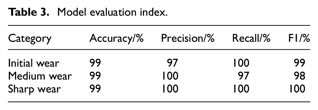
It can be seen from the figure that the performance of the data set in the training set and the validation set is similar, there is no over-fitting phenomenon, and a total of 30 generations of training. In the accuracy chart, when it runs to the seventh generation, the accuracy of the training set and the validation set are almost the same, and the accuracy reaches about 90%. After the 15th generation, the model accuracy tends to stabilize and converge, and the model accuracy is stable at around 98%; When the loss function curve is in the 5th generation, the loss values of the training set and the validation set are basically the same, the model starts to converge around the 10th generation, and the loss value is also stable at about 0.02; In the confusion matrix, intermediate wear and sharp wear can be fully identified, and only a small amount of data in the initial wear is not correctly identified. After the confusion matrix is obtained, the accuracy rate, precision rate, recall rate, and F1 index will be calculated to comprehensively judge the performance of the model. The model evaluation index is shown in Table 3.

Table 3.

Model evaluation index.

Category	Accuracy/%	Precision/%	Recall/%	F1/%
Initial wear	99	97	100	99
Medium wear	99	100	97	98
Sharp wear	99	100	100	100

Compared with traditional convolutional neural network

In the traditional convolutional neural network, only the convolution layer and the pooling layer are used. The size of the convolution kernel in the first layer is 5 × 1, and the number of convolution kernels is 64; the size of the convolution kernel in the second layer is 3 × 1, and the number of product cores is 128. The experiment uses the same experimental parameters and data set, and inputs the data into the traditional convolutional neural network. The obtained accuracy function curve is shown in Figure 13, and the loss function curve is shown in Figure 14.

Figure 13.

CNN accuracy curve.

Figure 14.

CNN loss function curve.

The x-axis is the number of iterations, and the y-axis is the accuracy. It can be seen from the figure that after many iterations, the accuracy of the model rises slowly, and finally only reaches 90%. The prediction accuracy of the model is not high.

It can be seen from the figure that the traditional convolutional network has some large fluctuations in the validation set during iteration, and the highest accuracy rate is about 90%. The loss function curve also has some fluctuations during iteration, and the loss value is at least 0.25. The data performance of the validation set is not very stable, which shows that the stability of the traditional convolutional neural network model is not good. In order to verify the performance of the model, other machine learning models are used for comparison, and the results are shown in the Table 4.

Table 4.

Comparison of different model indexes.

Network model	Training set accuracy/%	The validationset accuracy/%	Trainingset loss	The validationset loss
Traditional convolutional network	90.2	92.3	0.25	0.22
Residual convolutional network	98.7	98.5	0.08	0.05
SVM	89.1	87.6	0.62	0.59
BPNN	84.3	85.1	0.75	0.72

Comparison of different residual structures

In this paper, different residual blocks are used for comparison, and the different residual structures are shown in Figure 15. (a) means that there is only one residual block; (b) means that there are two residual blocks connected; (c) means that three residual blocks are connected. The experiments are carried out with the same dataset for verification, and the experimental results are shown in Table 5.

Figure 15.

Different number of residual block structures: (a) one residual block, (b) two residual blocks, and (c) three residual blocks.

Table 5.

Comparison of different residual structure indexes.

Networkmodel	Training setaccuracy/%	The validation set accuracy /%	Trainingtime /min
a	96.2	95.5	25
b	98.7	98.5	45
c	95.7	94.3	60

It can be seen from the table that the training effect of the deeper network model is not so good. The accuracy of the network model of the three residual blocks has a downward trend, and with the deepening of the network, the training time of the model continues to increase. Although the model with only one residual block has relatively less training time, the accuracy rate is not so high. Based on the above considerations, a convolutional neural network model with two residual structures is selected.

Conclusions

Conclusions 1: By analyzing the collected tool wear data, the tool wear curve is drawn by taking the maximum value of tool wear. Compared with the traditional convolutional neural network, BPNN and SVM, the convolutional neural network with residual connection proposed in this paper has faster training speed, higher accuracy of tool wear classification, and the accuracy is basically stable at about 98.5%.

Conclusions 2: The trained convolution neural network model has lower error, and the error of tool wear classification and recognition is only 0.1%, which is reduced by 0.15% compared with the traditional convolution neural network model. It can predict the wear state of the tool in advance and replace the tool in advance to avoid irreparable results caused by excessive wear.

Footnotes

Acknowledgements

Thanks to all the authors who have contributed to the paper.

Handling Editor: Chenhui Liang

Notations

TCM: Tool Condition Monitoring; BPNN: BP Neural Network; HMM: Hidden Markov Model SVM: Support Vector Machine; CNN: Convolutional Neural Network; BiLSTM: Bidirectional Long-Short-Term Memory; PCA: Principal Component Analysis.

Author contributions

Conceptualization, Y.W. and S.C.; methodology, J.L.; software, S.C.; validation, S.C.; formal analysis, Y.W.; investigation, Y.W.; resources, S.C.; data curation, J.L.; writing—original draft preparation, S.C.; writing—review and editing, S.C.; visualization, Y.W.; supervision, Y.W.; project administration, Y.W.; funding acquisition, S.C. All authors have read and agreed to the published version of the manuscript.

Declaration of conflicting interests

The author(s) declared no potential conflicts of interest with respect to the research, authorship, and/or publication of this article.

Funding

The author(s) disclosed receipt of the following financial support for the research, authorship, and/or publication of this article: “This research was funded by National Natural Science Foundation of Liaoning Province (LJKZ0532 and J2020108).

ORCID iD

Shengming Cheng

Data availability statement

The data presented in this study are available in this article.

References

Zhou

Xue

Review of tool condition monitoring methods in milling processes. Int J Adv Manuf Technol 2018; 96: 2509–2523.

Patra

Jha

Szalay

, et al. Artificial neural network based tool condition monitoring in micro mechanical peck drilling using thrust force signals. Precis Eng 2017; 48: 279–291.

Guo

Advances in monitoring technology of tool wear condition. Tool Eng 2019; 53: 3–13.

Zhu

Xie

. Tool wear state monitoring based on long-term and short-term memory neural network, vol. 12. Berlin: Springer, 2020. 703–712.

Bhuiyan

MSH

Choudhury

Nukman

Tool condition monitoring using acoustic emission and vibration signature in turning. Lect Notes Eng Comput Sci 2012; 2199: 531–538.

Cao

Application of improved CNN-LSTM model in rolling bearing application in fault diagnosis. Comput Syst Appl 2021; 30: 126–133.

Shen

Zhang

Deep hole boring tool condition monitoring based on long-term and short-term memory network. Modern Manuf Eng 2020; 08: 92–96.

Zhao

Wei

Research on fault diagnosis of rolling bearing based on Bilstm. Vibr Shock 2021; 40: 95–101.

Martins

CHR

Aguiar

Frech

, et al. Tool condition monitoring of single-point dresser using acoustic emission and neural networks models. IEEE Trans Instrum Meas 2014; 63: 667–679.

10.

Liu

Intelligent recognition of tool wear type based on convolution neural network. Comput Integr Manuf Syst 2020; 26: 2762–2771.

11.

Aghazadeh

Tahan

Thomas

Tool condition monitoring using spectral subtraction and convolutional neural networks in milling process. Int J Adv Manuf Technol 2018; 98: 3217–3227.

12.

Zhang

Sun

, et al. Recognition of tool wear state based on chaotic time series analysis method and support vector machine. Comput Integr Manuf Syst 2015; 21: 2138–2146.

13.

Tobon-Mejia

Medjaher

Zerhouni

CNC machine tools wear diagnostic and prognostic by using dynamic Bayesian networks. Mech Syst Signal Process 2012; 28: 167–182.

14.

Dai

Zhang

Meng

Support vector machine milling cutter wear prediction model based on deep learning and feature post-processing. Comput Integr Manuf Syst 2020; 26: 2331–2343.

15.

Krizhevsky

Sutskever

Hinton

GE.

ImageNet classification with deep convolutional neural networks. Commun ACM 2017; 60: 84–90.

16.

Lin

Research on tool wear condition monitoring technology based on deep learning. University of Science and Technology of China, 2017.

17.

Cao

Sun

Zhang

, et al. Online monitoring of tool wear based on convolutional neural network. Comput Integr Manuf Syst 2020; 26: 74–80.

18.

Zhang

Yao

Zhang

, et al. Tool wear monitoring method based on deep learning. Comput Integr Manuf Syst 2017; 23: 2146–2155.

19.

Ling

Wang

, et al. Online tool wear monitoring model based on long-short-term memory convolutional neural network. China Mech Eng 2020; 31: 959–1967.

20.

Chen

Xie

Yuan

, et al. Tool wear state monitoring method based on deep gated recurrent unit neural network. Computer Integr Manuf Syst 2020; 26: 1782–1793.

21.

Liu

Zhang

, et al. Tool wear monitoring using improved CNN-Bilstm model. China Mech Eng 2021; 3: 1–10.

22.

Tao

Zeng

Tool wear assessment based on regression tree and AdaBoost method. Comput Syst Appl 2017; 26: 212–219.

23.

Qin

Xie

Wang

Detection and control for tool wear based on neural network and genetic algorithm. Opt Precis Eng 2015; 23: 1314–1321.

24.

Xie

Duan

, et al. Monitoring of tool wear state based on principal component analysis and C-support vector machine. J Tongji Univ Natural Sci Ed 2016; 44: 434–439.

25.

Shi

Jiang

, et al. Prediction of tool wear and cutting force by the artificial neural network. Control Theory Appl 2018; 35: 1731–1737.

26.

Tamilselvan

Wang

Failure diagnosis using deep belief learning based health state classification. Reliab Eng Syst Saf 2013; 115: 124–135.

27.

Benkedjouh

Medjaher

Zerhouni

, et al. Health assessment and life prediction of cutting tools based on support vector regression. J Intell Manuf 2015; 26: 213–223.

28.

Zhao

Zhang

Improved CNN fault diagnosis of rolling bearing under variable working conditions. Journal of Xi’an Jiaotong Univ 2021; 12: 1–11.

29.

PHM Society. 2010PHM society conference data challenge. https://www.phmsociety.org/competition/phm/10.

Research on wear of Ni-Cr alloy milling based on residual network

Abstract

Keywords

Introduction

Tool wear monitoring framework

The establishment of one-dimensional convolutional network model

Convolutional layer

Pooling layer

The full connection layer

Residual structure

1D convolutional neural network batch normalization and regularization

Residual structured convolutional network model

Model training

Results

Experimental conditions

Experimental results

Compared with traditional convolutional neural network

Comparison of different residual structures

Conclusions

Footnotes

Acknowledgements

Notations

Author contributions

Declaration of conflicting interests

Funding

ORCID iD

Data availability statement

References