Sage Journals: Discover world-class research

Abstract

High-level wheel polygon wear is common in high-speed EMUs. Wheel polygon wear causes high-frequency vibration of vehicles and track systems, which seriously affects the safe operation of vehicles. Some key influencing factors are of great significance for restraining wheel polygon wear. In this paper, a long-term wear iterative model is established by combining the coupled vehicle/track dynamic model with the Archard wear model, which is used to simulate the whole development process of high-speed train wheel polygon. The development process of wheel polygon is simulated when the vehicle runs at 300 km/h. The simulating results are consistent with the actual situation. It is found that changing the speed of the vehicle can prevent the rapid development of the wheel polygon of a fixed order, so as to slow down the development of the wheel polygon. As the wheel hardness increases, the roughness level gradually decreases. If there is corrugation in the rail, it will greatly accelerate the development of wheel polygon, especially when the wavelength of rail corrugation can divide the wheel circumference. In addition, with the increase of rail corrugation amplitude, the promoting effect will gradually increase.

Keywords

Wheel polygon wear rail corrugation coupled vehicle/track dynamics model long-term wear iteration model

Introduction

Wheel polygon wear means that the wheel radius changes periodically or non-periodically along the entire circumference. Its wavelength is greater than 100 mm,^1,2 which is widely present in rail vehicles.^3,4 High-order wheel polygon wear causes many problems in rail and vehicle systems. On the one hand, the wheel polygons often produce high-frequency wheel/rail impact forces, resulting in damage or failure of bogie parts, which adversely affects the safety of the train. On the other hand, there is an acoustic resonance area within the frequency range of 300–400 Hz and 500–600 Hz in the rail vehicle body.

Regarding the causes of the wheel polygon, some scholars believe that the wheel polygon wear is mainly caused by bogie resonance. Under a certain speed condition, when the resonance wavelength can divide the circumference of the wheel, the wheel polygon wear enters a high incidence period.⁵ Other scholars believe that the resonance of track components and the dynamic interaction between the train and the track cause the wheel polygon.^6,7 These views still have great controversy and doubts among domestic and foreign research scholars. It needs to be further verified from theory and experiment to clarify the factors affecting the formation and development of wheel polygon wear, and countermeasures need to be proposed to solve the wheel polygon problem.

Johansson⁸ and Zobory⁹ finished a comprehensive study on wheel and track wear problems, and conducted a literature review of numerical methods for wheel wear prediction, and summarized a long-term wear iteration model. Brommundt¹⁰ built a simple wheel-track model that delved into the mechanism of wheel polygon formation and found that wheel-track interactions and wheelset moment of inertia are the root causes of polygon intensification. Meinke and Meinke¹¹ built a 40-degree-of-freedom wheelset model using rotor dynamics theory to simulate the gradual polygonization of the original ideal wheel under excitation forces to analyze the effect of disk brakes on wheel polygonization. Wu et al.¹² established a numerical model of wheel polygon wear and simulated the development process of wheel polygons. By analyzing the frequency response between wheel and rail, they found that the third-order vertical bending resonance of the rail between wheels may cause wheel polygons. The high-order polygon abrasion of high-speed train wheels will cause strong high-frequency vibration of the axle box. Li¹³ analyzed the transfer relationship of high-frequency vibration from the axle box to the vehicle body bolster. As a result, the wheel polygon has a great impact on the axle box, which may cause the axle box end cover bolts fall off, and may resulting in safety problems.

The main purpose of this article is to study the factors affecting the development of wheel polygon wear from the perspective of practical applications, and then propose corresponding restraining measures. This is of very important practical significance. A vehicle/track coupling dynamics model was established using SIMPACK, in which the wheelset and the rail were set as flexible bodies. The Archard wear model was established using MATLAB. In this paper, a long-term wear iterative model is established through the joint simulation of SIMPACK and MATLAB. The whole process of the generation and development of high-speed train wheel polygons was simulated, and from the perspective of the entire development process of wheel polygons, some influencing factors of wheel polygons were studied and discussed in detail, and some practical results were also obtained.

Establishment of long-term wear iteration model

Archard wear model

The Archard wear model has been widely used in calculating wheel tread wear, and the calculated results are more consistent with the actual situation. Therefore, the Archard model can be also used for calculating wheel polygon wear. The Archard wear equation is:

V_{wear} = K_{w} \frac{Nd}{H}

(1)

In the equation, $V_{wear}$ is the volume of wear material. d is the sliding distance. N is the normal contact force. H is the hardness of the softer material of the two contacting objects. $K_{w}$ is the wear coefficient and the value is dependent on the contact normal pressure and the slip velocity. For tread wear, the wear coefficient is in the range of $1 \times 10^{- 4} ~ 10 \times 10^{- 4}$ . For wheel flange wear, the wear coefficient is in the range of $1 \times 10^{- 4} ~ 400 \times 10^{- 4}$ . In this paper, a straight track is chosen and simulated, and the wheel-rail slip is relatively small, so the wear coefficient can be assumed to be $1 \times 10^{- 4}$ .

It can be known from Hertz contact theory that the wheel-rail contact patch has an elliptical shape. Kalker extracted parameters of a and b from Hertz theory, and proposed a compressive stress distribution that is more suitable for wheel-rail contact analysis.^14,15 The calculation formula of normal stress distribution in Hertz contact theory is shown in equation (2). This stress distribution is semi-ellipsoidal.

p_{z} = \frac{3 N}{2 π ab} \sqrt{1 - {(\frac{x}{a})}^{2} - {(\frac{y}{b})}^{2}}

(2)

The relative sliding speed at the point (x, y) where the wheel contacts the rail can be calculated by FASTSIM algorithm. As shown in equation (3).

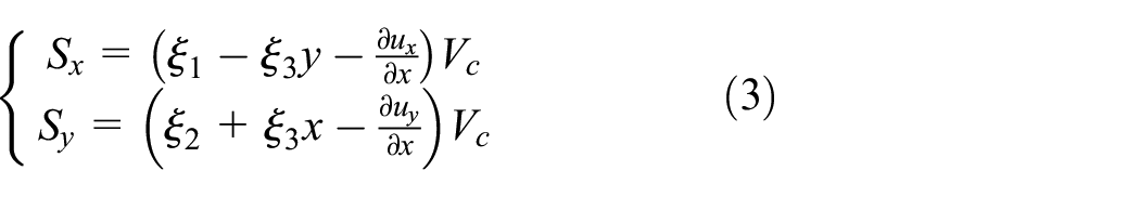
{\begin{matrix} S_{x} = (ξ_{1} - ξ_{3} y - \frac{\partial u_{x}}{\partial x}) V_{c} \\ S_{y} = (ξ_{2} + ξ_{3} x - \frac{\partial u_{y}}{\partial x}) V_{c} \end{matrix}

(3)

In the equation, the longitudinal direction refers to the direction of travel of the vehicle, and the lateral direction refers to the direction of vehicle lateral movement. $S_{x}$ and $S_{y}$ represent the longitudinal and lateral sliding speed respectively. $ξ_{1}, ξ_{2}, ξ_{3}$ are longitudinal, lateral and spin creep rates. $u_{x}, u_{y}$ are the longitudinal and lateral elastic sliding amounts. $V_{c}$ is the running speed of the vehicle.

Then the FASTSIM algorithm is combined with the Archard wear model to calculate the wear distribution in the contact patch.

Δ z (x, y) = \frac{K_{w}}{H} \cdot p_{z}^{'} \cdot \sqrt{S_{x}^{2} + S_{y}^{2}} \cdot \frac{Δ x}{V_{c}}

(4)

In the equation, $Δ z (x, y)$ is the wear depth of the unit where central coordinates are (x, y). $Δ x$ is the longitudinal length of the grid on the contact patch.

MATLAB software is used to write a program to establish a wear model, and the dynamic data are calculated and obtained by using the vehicle/track dynamic model. After that, the data will be used in the wear model. Then the wear depth distribution in the contact patch is calculated and shown in Figure 1. In the distribution diagram of wear depth, it is divided into wear area and non-wear area. The wear area is the creep zone, the non-wear area is the adhesive zone. The wear will begin to happen from the junction of the adhesion zone and creep zone. And the wear depth tends to be 0 at the other end of creep zone.

Figure 1.

Distribution of wear depth in contact patch.

Coupled vehicle/track dynamic model

Because the excitation frequency of the wheel polygon is usually high and the frequency covered by the traditional multi-rigid body dynamic model is limited, which is difficult to meet the simulation requirements. Therefore, this paper combines the finite element software ANSYS and the multi-body dynamics software SIMPACK to establish a vehicle/track coupling dynamic model, which considers flexible wheelsets and flexible tracks.¹⁶

This paper takes a certain type of high-speed train as the research object and uses the multi-body dynamics software SIMPACK to establish a multi-rigid-body dynamics model. The dynamic model includes one car body, two frames, four wheelsets, and eight axle boxes with a total of 50 degrees of freedom. Among them, the body, frame, and wheelset all consider the freedom of the six directions of horizontal, vertical, longitudinal, nodding, shaking and rolling, and the axle box only considers the freedom of the nodding direction. The finite element model of the wheelset is established by using the finite element software ANSYS. The wheel and the axle are regarded as an integral component, and the interference fit relationship between the wheel and the axle is not considered. The wheelset is hexahedral meshed, and the element type is 3D solid element solid45. The 648 main degree of freedom points on the wheelset are selected for substructure analysis, and the analyzed flexible wheelset is imported into SIMPACK. Then, the custom reference point method in SIMPACK is used to rigidly hinge the main degrees of freedom at the axle box connection and the marker points at the shaft hollow position, and is used to replace the rigid wheelset. The modal superposition processing is performed on the wheel, and 30-order free modes are added to the finite element model of the wheel, and the maximum modal frequency reaches 900 Hz. The mode includes wheel bending mode, axle disk torsion mode, axle second bending mode, axle third bending mode, and axle fourth bending mode. Modal superposition processing is also performed on the rail, and 50-order free modes are added to the finite element model of the rail, and the maximum modal frequency reaches 1500 Hz. These include the first, second, and third-order vertical bending modes of the rail, and pinned-pinned resonance.

The establishment of the flexible track not only needs to establish the finite element model of the rail, but also needs to write the configuration file of the flexible track. The configuration file is read through the FLEXTRACK module in the SIMPACK software to realize the import of flexible tracks. The structures under the rails, fasteners, track beds and other rails are uniformly simulated by spring damping elements. The front and end of the track are fixed with large stiffness and large damping force elements. The parameter settings are shown in Table 1.

Table 1.

The main parameters of the model.

Parameters	Values
Wheel profile	S1002CN
Wheel radius	0.46 m
Wheelbase	2.5 m
Rail profile	60 N
Sleeper spacing	0.63 m
Young’s modulus of rail	$2.1 \times 10^{11} N / m^{2}$
Poisson’s ratio of rail	0.3
Density of rail	$7850 kg / m^{3}$
Friction coefficient	0.3
Support stiffness of the rail pad	20 MN/m
Damping coefficient of the rail pad	30 kNs/m

Wear prediction

For a certain point on the wheel’s rolling circle, it will go through the process of entering the contact patch – adhesion zone – creeping zone – leaving the contact patch during the wheel rotation. Therefore, in this paper, the wear amount on the contact spot is superimposed longitudinally to represent the total wear amount caused by a certain point on the rolling circle of the wheel during one revolution of the wheel. Hence, it is necessary to longitudinally superimpose the wear on the wheel-rail contact patch. Since this article only studies the running of the vehicle on a straight track, the lateral displacement of the wheelset is small, so this article does not consider the lateral displacement of the wheelset. Assuming that the center of the wheel-rail contact patch is always located on the wheel’s rolling circle, and in order to make the calculation results general, and the average wear is superimposed along the transverse direction to represent a rotating wheel passing through the wheel rolling circle. This article only studies the wear of the wheel’s nominal rolling circle on the circumference, and assumes that the wheel tread does not change due to wear. The calculation equation is shown in equation (5).

Δ z^{k} = \frac{\sum_{i = 1}^{MM} \sum_{j = 1}^{NN} Δ z (i, j)}{NN}

(5)

In the equation, $Δ z^{k}$ is the depth of wear of the discrete point numbered k on the rolling circle. $Δ z (x, y)$ is the wear depth of the grid numbered i along the longitudinal direction and numbered j along the lateral direction on the contact patch. MM is the number of grids divided along the longitudinal direction, and NN is the number of grids divided along the horizontal direction.

In order to study the wear distribution on the circumference of the wheel, and the wheel hub is divided into 3600 sampling points, with an interval of 0.1°. After calculating the wear of these 3600 sampling points and fitting it with a 40-order Fourier series, the wear on the wheel circumference can be obtained.

In order to improve calculation efficiency, it is assumed that the wheel polygon has multiple time scales, which means that the scale factor is applied to the results of short-term dynamic simulation to simulate the wear effect that occurs on a longer time scale. That is, the wear caused by short-distance driving is multiplied by a scale factor to simulate the wear caused by long-distance driving. Generally speaking, this distance is about 1000 km or less. In this paper, the time scale is set to $2 \times 10^{5}$ , which corresponds to the polygon wear under 578 km.

This paper only studies the operation of the vehicle on a straight track, and inputs the measured initial wheel polygon into the long-term wear iteration model, without considering the influence of track irregularity. The initial wheel irregularity of the wheel is added in the calculation, but the irregularity of the rail is not added. This is because the excitation provided by the initial wheel irregularity is periodic when calculating the wheel polygon wear, which may lead to the generation of the wheel polygon. However, the excitation of rail irregularities is random and contributes little to the wheel polygon. This model simulates the development process of the wheel polygon when the vehicle travels at a speed of 300 km/h, and shows the change of the wheel radius during the iteration process, as shown in Figure 2. It can be found from Figure 2 that when the driving speed is 300 km/h, the wheel radius gradually becomes a wavy curve. Figure 3 shows the comparison of the measured and calculated irregularities. The wheel polygon wear measured data is obtained when CRH380B EMU runs about 150,000 km on China’s Beijing Shanghai high speed rail at the speed of 300 km/h. Due to the high-speed running of the vehicle, the railway is dominated by straight lines and large radius curves, and the lateral movement of the wheels is small at this time. Therefore, in the study of wheel polygon wear, only the calculation results of straight-line condition are consistent with the actual situation to a certain extent. It can be seen from Figure 3 that the measured and calculated irregularities are very similar, and they both have obvious harmonic wear.

Figure 2.

Change of wheel radius.

Figure 3.

Comparison of measured and calculated irregularities.

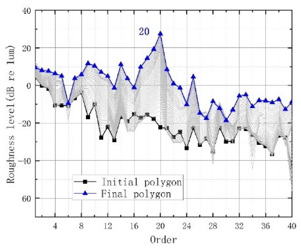
Generally, the roughness grade is used to describe the irregularity of the wheel circumference. First, a 40-order Fourier series is required to fit the wheel polygon. Because the order of the wheel polygon generally does not exceed the order of 30, it is sufficient to use the 40-order Fourier series to fit it. Then the wheel roughness level calculation equation is used to obtain the order change of the wheel surface roughness. The formula for calculating the roughness level is shown in formula 6, and the polygon sequence change of the wheel is shown in Figure 4.

L_{a}^{k} = 10 \log {(\frac{r_{k}}{r_{ref}})}^{2} = 20 \log (\frac{A}{\sqrt{2}})

(6)

Figure 4.

Roughness level.

In the equation, $L_{a}^{k}$ is the roughness level, k is the order, the value is from 1 to 40. A is the amplitude of the function.

It can be seen from Figure 4 that when the train travels at a speed of 300 km/h, the wheel polygons develop from the initial non-obvious high-order polygons to finally 20-order. The order spectrum of wheel harmonic wear is shown in Figure 5. From Figure 5, it can be seen that the measured and calculated results are dominated by 20-order polygons, and the calculated results are consistent with the measured results. This phenomenon verifies the correctness of the long-term wear iteration model.

Figure 5.

Comparison of measured and calculated roughness.

Research on the influencing factors of wheel polygon

The generation and development of wheel polygon wear is a complex and long-term process, with many influencing factors. Both field experiments and laboratory experiments have significant limitations, and these influencing factors cannot be identified individually. Therefore, it can only be studied through simulation. This paper uses a long-term wear iterative model to simulate the generation and development of wheel polygons when the train runs at 300 km/h. The results are consistent with the actual situation. Therefore, the model can be used to study the influence of train running speed, wheel surface roughness and rail corrugation on the development of wheel polygons.

Vehicle speed changes

According to the actually measured data and simulation results, when the train is running at speeds of 300 km/h, the wheel polygon has developed from the initial non-polygon to the dominant order of 20. According to the frequency calculation equation, the excitation frequency generated by the polygon is about 580 Hz, indicating that there is a fixed vibration frequency between the vehicle and the track system. This 580 Hz vibration frequency has promoted the generation and development of wheel polygons.

The frequency calculation equation is shown below.

f = \frac{n \cdot v}{2 π r}

(7)

In the above equation, f is the excitation frequency caused by the polygon. v is the speed of the train. r is the radius of the wheel. From the frequency calculation equation, it can be found that the final order of the wheel polygon is related to the running speed of the vehicle. With the change of running speed, the dominant order of polygon will change. Theoretically, with the increase of vehicle speed, the dominant order of wheel polygon will decrease, which is consistent with the real situation. In addition, when the vehicle keeps running at a certain speed, the corresponding wheel polygon order will develop rapidly. Therefore, during vehicle operation, by adjusting the running speed, the rapid growth of wheel polygon of a certain order can be prevented, and consequently to achieve the purpose of restraining the rapid growth of polygon wear.

In order to study the influence of the change of running speed on wheel polygon wear, this paper arranges five speed levels of 280, 290, 300, 310, and 320 km/h respectively, and sets four operating conditions:

The vehicle runs at a fixed speed of 300 km/h.

The vehicle increases step by step with five speed levels. After 1/5 of the total mileage of each speed level, it enters the next speed level. In each process, the wheel polygon needs to be iterated 10 times.

Similar to the second condition, the difference is that the running speed of the vehicle decreases gradually.

The five speed levels of vehicle running speed change randomly.

The calculation results are shown in Figures 6 and 7. Figure 6 is the change of roughness level order under four working conditions.

Figure 6.

Change of roughness level order under four working conditions: (a) fixed speed, (b) random speed, (c) speed decreases step by step, and (d) Speed increases step by step.

Figure 7.

Comparison of four roughness levels.

It can be seen from Figures 6 and 7 that the dominant order of polygon wear is 20 and the roughness level is 26 dB when the vehicle runs at 300 km/h. The results show that the roughness level of polygon is basically the same as that of gradual increase and gradual decrease, both of which are around 20 dB, and the dominant order is 21 and 19 dB, respectively, which may be related to the initial running speed of vehicles. When the vehicle speed changes randomly, the polygon roughness level is around 15 dB. From the analysis of the above calculation results, it can be seen that the growth rate of high-order wheel polygon can be restrained by changing the running speed frequently.

Wheel hardness

According to the Archard wear equation, the wear volume of the wheel surface is inversely proportional to the hardness of the wheel surface. Therefore, it can be inferred that when the wheel shows greater hardness, the wear depth is smaller. Generally speaking, the wheel hardness will gradually become smaller as the wheel radius decreases, and the wheel hardness is in the range of 300HB to 360HB. Therefore, this paper studies the development of wheel polygon wear when the wheel hardness is 300, 320, and 350HB.

The long-term wear iterative model is adopted, with the initial wheel polygon as the input. Figure 8 shows the development process of wheel roughness levels with different wheel hardness obtained by this method. It can be seen from Figure 8 that the change of wheel hardness does not change the main order of the final wheel polygon. The final roughness level comparison is shown in Figure 9. When the wheel hardness is 320 HB, the final roughness level is almost the same as the hardness of 300 HB. However, when the wheel hardness is 350 HB, the final roughness level is significantly lower than the 300 HB hardness. Therefore, a substantial increase in the surface hardness of the wheel can decrease the roughness level, which would gradually decrease with the rise of wheel hardness.

Figure 8.

Change of roughness level of wheels with different hardness: (a) 300 HB, (b) 320 HB, and (c)350 HB.

Figure 9.

Comparison of roughness levels of different hardness.

Wavelength of rail corrugation

Rail corrugation is a kind of rail vertical irregularity, which is distributed on the wheel/rail contact surface longitudinally along the rail. Rail corrugation and wheel polygonal wear characteristics are very similar, only the wear carrier is different, so there may be some relationship between the two kinds of wear. The wheel/rail contact model plays an important role in connecting the vehicle and track subsystem. In this study, the measured rail corrugation is generally distributed on the rail surface with irregular wavelength and amplitude, and the wavelength is generally 120–160 mm, which is bigger than 10 times the axis length of the contact patch. The Hertz theory is still valid in evaluating the normal force between the wheel and rail. In the simulation calculation, it is usually treated as a periodic sine wave, which is represented by the following equation.

z_{rw} = d_{p} \sin (2 π \frac{x_{rw}}{λ} + φ)

(8)

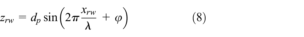
In the equation, $z_{rw}$ is the vertical position of rail corrugation, $d_{p}$ is the amplitude, $λ$ is the wavelength, $x_{rw}$ is the longitudinal position of the rail, $φ$ is the initial phase angle of the sine wave.

In order to study the influence of rail corrugation on the development of wheel polygons, nine kinds of rail corrugation with fixed wavelengths are set up in this paper. The wavelengths are 135, 137, 140, 142, 145, 147, 150, 152, and 155 mm respectively. In addition, a rail corrugation with five wavelengths of 135, 140, 145, 150, and 155 in sequence is set up, with an average wavelength of 145 mm. The amplitude of rail corrugation is set to 0.01 mm and the initial phase angle is 0. Taking the measured initial wheel polygon as input, the rail corrugation is only considered in the track irregularity, and the vehicle running speed is set at 300 km/h. The development process of wheel polygon iteration with five times is calculated by using the long-term wear iterative model. The change of wheel radius corresponding to rail corrugation of 9 fixed wavelengths and 1 mixed wavelength is shown in Figure 10(a) to (j). The change of wheel radius with five iterations without rail corrugation is shown in Figure 11.

Figure 10.

The change of wheel radius at different wavelengths: (a) 135 mm, (b) 137 mm, (c) 140 mm, (d) 142 mm, (e) 145 mm, (f) 147 mm, (g) 150 mm, (h) 152 mm, (i) 155 mm, and (j) mixed wavelength.

Figure 11.

The change of wheel radius without rail corrugation.

It can be seen from Figures 10 and 12 that when there are rail corrugations on the rail, the shape of the wheel gradually changes to a high-order polygon. With the different wavelength of rail corrugation, the order of wheel polygon wear is also different. From Figure 11, it can be found that when there is no rail corrugation on the rail, the development of the wheel polygon is relatively slow. This shows that if there is rail corrugation in the rail, the development speed of high-order wheel polygon will be greatly promoted.

Figure 12.

Comparison of roughness levels at different wavelengths.

From the above calculation results, it can be found that the promotion effect of rail corrugation with different wavelengths on wheel polygon is different. The main order and roughness level of wheel polygon under different wavelengths are shown in Table 2.

Table 2.

Main order and roughness level of wheel polygon at different wavelengths.

Wavelength (mm)	Order	Roughness level(dB re 1 µm)
135	21	6.87
137	21	13.08
140	21	12.53
142	20	8.25
145	20	13.43
147	20	13.03
150	19	9.0
152	19	12.36
155	19	11.95

It can be seen from Table 2 that the dominant order and roughness level of wheel polygon are different due to different wavelength. After analyzing the calculation results, it is found that the cause of this phenomenon may be related to whether the wavelength of rail corrugation can divide the circumference of wheel. The division relationship between wheel circumference and wavelength is shown in Table 3.

Table 3.

Wavelength and ratio of wheel circumference to wavelength.

Wavelength (mm)	Ratio	Round to thewhole number
135	21.41	21
137	21.09	21
140	20.64	21
142	20.35	20
145	19.93	20
147	19.66	20
150	19.27	19
152	19.01	19
155	18.65	19

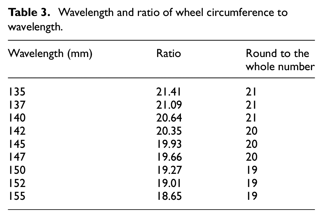
It can be found from Table 3 that the wheel circumference can be divided by the wavelengths of 137, 145, and 152 mm. In addition, it can be found that the order of wheel polygon has a certain corresponding relationship with the wavelength of rail corrugation. The relationship between ratio and roughness level is shown in Figure 13. As shown in Figure 13, there are three peaks in the roughness level. When the ratio is 19, 20, and 21, the roughness level reaches the peak. This shows that when the wavelength of rail corrugation can divide the wheel circumference, the wheel polygon can develop more rapidly.

Figure 13.

Ratio of wheel circumference to wavelength and roughness level.

Amplitude of rail corrugation

Through the research on the influence of the wave length of rail corrugation on the development of wheel polygon, it is found that rail corrugation can promote the development of wheel polygon when the amplitude of rail corrugation is 0.01 mm. However, as the actual measured amplitude of rail corrugation is not fixed, and most of the amplitude changes in the range of 0–0.03 mm. Therefore, in order to study the influence of rail corrugation amplitude on the development of wheel polygon, three wavelengths of 137, 145, and 152 mm are chosen in this paper. The long-term wear iterative model is used to simulate the development of wheel polygon when the rail corrugation amplitude is 0.005, 0.01, and 0.02 mm respectively. The results are shown in Figures 14 to 16.

Figure 14.

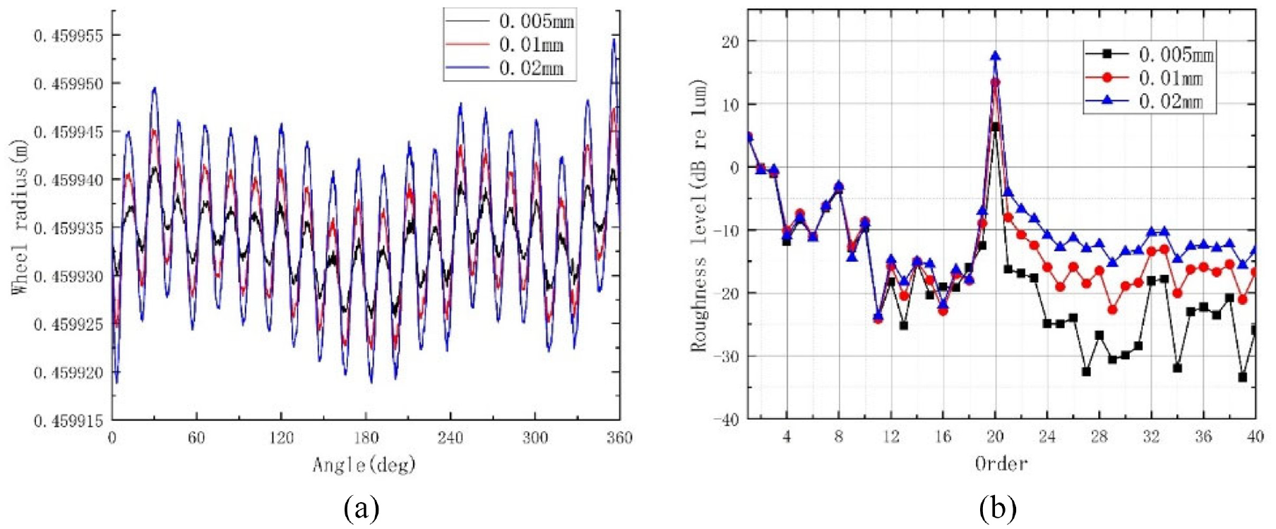
When the wavelength is 137 mm, the influence of amplitude change on wheel polygon: (a) wheel radius and (b) roughness level.

Figure 15.

When the wavelength is 145 mm, the influence of amplitude change on wheel polygon: (a) wheel radius and (b) roughness level.

Figure 16.

When the wavelength is 152 mm, the influence of amplitude change on wheel polygon: (a) wheel radius and (b) roughness level.

Figures 14 to 16 show the comparison of wheel radius and wheel roughness level under different amplitudes when the wavelength is 137, 145, and 152 mm respectively. It can be seen from Figures 14(a), 15(a) and 16(a) that the amplitude of final wheel radius increases with the rise of rail corrugation amplitude. According to Figure 14(b), when the rail corrugation amplitude is 0.005, 0.01, and 0.02 mm, the final wheel roughness is 5.3, 13.1, and 17.1 dB respectively. According to Figure 15(b), when the rail corrugation amplitude is 0.005, 0.01, and 0.02 mm, the final wheel roughness is 6.4, 13.4, and 17.5 dB severally. According to Figure 16(b), when the rail corrugation amplitude is 0.005, 0.01, and 0.02 mm, the final wheel roughness is 5.3, 12.4, and 16.5 dB respectively. The above results show that when the wavelength is fixed, the increase of rail corrugation amplitude will promote the development of wheel polygon, which is also consistent with the actual situation.

Conclusions

The coupled vehicle/track dynamic model including flexible wheelset and flexible track is established, and the long-term wear iterative model is established by combining the dynamic model with the Archard wear model through the joint simulation of MATLAB and SIMPACK. The long-term wear iterative model are used to study the influence of speed change, wheel hardness and rail corrugation on wheel polygon development from the perspective of the whole development process of wheel polygon.

The long-term wear iterative model is used to simulate the whole development process of wheel polygon when the vehicle running speed is 300 km/h. It is found that the wheel polygon has developed from no obvious high-order polygon at the beginning to 20 order polygon. This phenomenon is similar to the wheel polygon generated in the actual train operation process, which verifies the correctness of the long-term wear iterative model.

Changing the speed of the vehicle can slow down the development of wheel polygons, but the way how the speed of the vehicle changes is related to the degree of restraining of high-order wheel polygons. The method of random speed change curbs the wheel polygon better than the method of gradually increasing and decreasing speed.

The change of wheel hardness does not change the main order of the wheel polygon, but it can change the roughness level. The study found that as the wheel hardness increases, the roughness level gradually decreases too.

Rail corrugation and wheel polygonal wear characteristics are very similar, only the wear carrier is different. It is found that if the vehicle runs on the track with rail corrugation, the development of wheel polygon will be greatly promoted. When the wavelength of rail corrugation can divide the wheel circumference, the promotion of wheel polygon will be greater. And with the increase of rail corrugation amplitude, the promoting effect on wheel polygon also increases gradually.

Footnotes

Handling Editor: Chenhui Liang

Declaration of conflicting interests

The author(s) declared no potential conflicts of interest with respect to the research, authorship, and/or publication of this article.

Funding

The author(s) disclosed receipt of the following financial support for the research, authorship, and/or publication of this article: NSFC high speed railway joint fund (U1734201): Project of science and technology research and development plan of China National Railway Group Co., Ltd (N2018G044).

ORCID iD

Zhi-kun Song

References

Chi

. Influence of polygonal wear of railway wheels on the wheel set axle stress. Veh Syst Dyn 2015; 53: 1535–1554.

Chi

Gao

. Damage tolerances of a railway axle in the presence of wheel polygonalizations. Eng Fail Anal 2016; 66: 44–59.

Barke

Chiu

. A review of the effects of Out-Of-Round wheels on track and vehicle components. Proc IMechE, Part F: J Rail and Rapid Transit 2005; 219: 151–175.

Liu

Zhai

. Analysis of vertical dynamic wheel/rail interaction caused by polygonal wheels on high-speed trains. Wear 2014; 314: 282–290.

Jin

Fang

, et al. An investigation into the mechanism of the polygonal wear of metro train wheels and its effect on the dynamic behaviour of a wheel/rail system. Veh Syst Dyn 2012; 50: 1817–1834.

Popp

Kruse

Kaiser

. Vehicle-track dynamics in the mid-frequency range. Veh Syst Dyn 1999; 31: 423–464.

Johansson

Andersson

. Out-of-round railway wheels—a study of wheel polygonalization through simulation of three-dimensional wheel–rail interaction and wear. Veh Syst Dyn 2005; 43: 539–559.

Johansson

. Out-of-round railway wheels - literature survey, field tests and numerical simulations. Licentiate Thesis, Chalmers University of Technology, Göteborg, Sweden, 2003.

Zobory

. Prediction of wheel/rail profile wear. Veh Syst Dyn 1997; 28: 221–259.

10.

Brommundt

. A simple mechanism for the polygonalization of railway wheels by wear. Mech Res Commun 1997; 24: 435–442.

11.

Meinke

. Polygonalization of wheel treads caused by static and dynamic imbalances. J Sound Vib 1999; 227: 979–986.

12.

Rakheja

Cai

, et al. A study of formation of high order wheel polygonalization. Wear 2019; 424–425: 1–14.

13.

. Mechanism study of wheel polygonization based on modal analysis of rail. 2017.

14.

Jin

Liu

. Tribology of wheel and rail. Beijing: China Railway Publishing House, 2004.

15.

Vollebregt

EAH

Wilders

. FASTSIM2: a second-order accurate frictional rolling contact algorithm. Comput Mech 2011; 47: 105–116.

16.

Zhikun

Yinqing

, et al. Research on vibration characteristics of wheel-rail corrugation under flexible wheel and rail. J China Railw Soc 2018; 40: 33–40.

Study on the influencing factors in the development process of high-speed train wheel polygon