
Abstract
In this work, numerical simulations of upward turbulent bubbly flows in vertical pipes are conducted in the Euler-Euler framework with a low-Reynolds-number (LRN) model for liquid. It is found that the existing correlation for the drag coefficient of a single bubble in a shear flow, which has been successfully used along with the high-Reynolds-number (HRN) models, cannot be used with the LRN model. The reason is that drag forces of bubbles calculated using such correlation are enormous in near-wall cells (order of
Introduction
Turbulent bubbly wall-confined vertical flows have many important industrial applications, such as in gas-liquid chemical reactors, boilers, airlift pumps and oil production and transport. The presence of bubbles in these flows can significantly influence skin friction compared to single-phase liquid flow, increasing mixing and heat transfer between phases. Owing to these reasons these flows have been extensively studied in the last 40 years. However, due to the great complexity of bubble-liquid and bubble-bubble interactions and the presence of wall confinement, the study of these flows still represents a challenge for researchers.
Direct numerical simulation studies with interface tracking of every bubble provide the highest level of numerical description of turbulent bubbly flows (Lu and Tryggvason,1,2 Adoua et al., 3 Bois and du Cluzeau 4 ). However, due to high computational expense, at the present, these studies are possible for relatively low Reynolds number flows with limited number of bubbles (around few hundreds at most).
Due to the reasonable computational price of large-scale computations, most numerical studies in the Euler-Euler framework for upward turbulent bubbly flows in vertical pipes (Hosokawa and Tomiyama, 5 Lubchenko et al., 6 Magolan et al., 7 Parekh and Rzehak, 8 Colombo et al., 9 Lopez de Bertodano et al., 10 Rzehak and Krepper,11–14 Rzehak and Kriebitzsch, 15 Rzehak et al., 16 Troshko and Hassan 17 ) are conducted using high-Reynolds-number (HRN) models for liquid phase. In these models, the turbulence in the near-wall region is modelled using various empirical equations known as wall functions, and boundary conditions for the momentum and turbulence transport equations are specified somewhere in the near-wall region, and not at the wall itself.
There is no clear conclusion if wall functions in the context of two-phase flows should always be the same as in single-phase flows (Troshko and Hassan, 17 Colin et al. 18 ). Still, if a HRN model is used in Euler-Euler numerical studies of wall confined turbulent bubbly flows, wall functions used for single-phase flow are usually applied without any change.
Alternatives to HRN models are low-Reynolds-number (LRN) models, which fully resolve flow fields up to the wall. Since many physical quantities have strong gradients in near-wall region, the mesh resolution in LRN approach has to be high enough to capture these changes (
In the upward turbulent bubbly flows, due to the buoyancy that affects the bubbles, air velocity is higher than water velocity. This difference in phase velocities modifies the turbulence intensity in the liquid phase. This can be taken into account by including source terms (BIT models) in the single-phase two-equation turbulence models. These source terms are modelled but, no consensus for their form has been reached yet (Magolan et al. 7 ). Rzehak and Krepper 13 have reported a comparison of different BIT models. They found that it is difficult to report general conclusions and that further research on this topic is needed. To reach a general solution, they proposed two directions: the first, the formation of a more complex BIT model, and the second, the introduction of a separate equation for the bubble-induced turbulent kinetic energy (Chahed et al. 19 ).
A problem that occupies the most attention, when simulating a two-phase flow, is the modelling of interfacial forces. They reproduce the different physical effects that are part of the momentum interfacial exchange between phases.
There are many models of interfacial forces. Different models were developed based on the analysis of sets of experimental results that belong to a specific experimental case. For such or similar cases, these models will predict the results well numerically, but when trying to apply these models to a case that differs significantly from that used to optimise the model, unsatisfactory results are frequently obtained. This means that generalised interfacial force models, that will give good results in various cases of two-phase flow, still do not exist. For each force model, it is necessary to know what its area of application is. The modelling of these interfacial forces is still an open question.
In upward turbulent bubbly flows the radial distribution of void fraction depends on the competition between lateral forces – lift force, turbulent dispersion force and wall lubrication force. The wall lubrication force affects the flow in the distance of less than one half bubble diameter from the wall. Outside this area, the void fraction profile is determined by the ratio of the turbulent dispersion force and the lift force. Shawkat et al. 20 shows that it is very difficult to distinguish the conditions under which a wall peak or core peak void fraction profile occurs in bubbly flows and that it depends on numerous parameters such as the ratio of volumetric fluxes of phases, the ratio of pipe diameter and bubble diameter, slip ratio, Eötvös number…
Accurate determination of the bubble drag coefficient is of great importance for the successful simulation of two-phase bubbly flow, since the drag force is the dominant interfacial force in the streamwise direction. The unsteady, three-dimensional flow around a spherical bubble moving steadily in viscous linear shear is analysed numerically by Legendre and Magnaudet 21 by solving full Navier-Stokes equations. They found that the drag coefficient of a single bubble in a shear flow increases with the increase in the ratio between the liquid velocity difference across the bubble and the relative velocity of gas and liquid. This increase in the drag coefficient is caused by pressure modification around the bubble.
Hosokawa and Tomiyama 5 studied experimentally and numerically (with HRN models) upward turbulent bubbly flow in a vertical pipe. They found that the application of a correlation proposed by Legendre and Magnaudet 21 for a drag coefficient of a single bubble in shear flow in numerical simulations reduces the relative velocity of gas and liquid. This led to a better agreement of experimental and numerical results.
The present study examines upward turbulent bubbly flows in the Euler-Euler framework using the LRN model for liquid. To the authors’ knowledge, up to now, there are a limited number of such studies (Colombo and Fairweather, 22 Colombo et al. 9 ). Also, there is no paper in the available literature to verify the effect of the drag coefficient of a single bubble in the shear flow in combination with LRN models in upward turbulent bubbly flows in vertical pipes. This paper aims to achieve this.
Description of a numerical method
Governing equations of two-phase flows
Using the index

and

where
Modelling of interfacial force
In this paper, the interfacial force

where
Drag force
The drag force is given by:
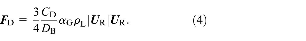
The drag coefficient

where:

where the bubble Reynolds number


To account for the effect of shear rate on the increase in drag coefficient of a single spherical bubble, Legendre and Magnaudet 21 proposed the following correlation:

where

and
Equation (10) is plotted in Figure 1, together with corresponding experimental data from Hosokawa and Tomiyama. 5

Dependence of the ratio of bubble drag coefficient in shear flow ) experimental data from Hosokawa and Tomiyama
5
; ( ) equation (10) of Legendre and Magnadeut
21
; (
) equation (10) of Legendre and Magnadeut
21
; ( ) proposed equation (12). The dependence is shown for different ranges: (a) up to the 2 and (b) up to the 20.
The agreement of equation (10) against experimental data is relatively good for non-dimensional shear rate
With respect to equation (11), the non-dimensional shear rate
If the flow is analysed in the context of LRN models, the centroids of the adjacent wall cells are at very small distance from the wall. In typical simulations in the Euler-Euler framework of upward turbulent bubbly flows in vertical pipes with a LRN model for liquid and bubble drag coefficient defined by the equation (10), it is observed that drag force on a single bubble can achieve values of order
This analysis leads to the conclusion that the drag coefficient of a single bubble in shear flow given by equation (10) of Legendre and Magnaudet
21
cannot be used along with the LRN models. On the other hand, equation (10) can be used with HRN models, since the centroids of the adjacent wall cells are at much greater distance from the wall (
To avoid extremely large values of bubble drag coefficient predicted by equation (10) near the wall in the context of LRN models, we propose the following correlation for the drag coefficient of a single bubble in a shear flow, based on linear regression with experimental data of Hosokawa and Tomiyama 5 :

where it is assumed
It can be seen in equation (12) that the dependence of the new correlation on
Lift force
The lift force is given by:

where

where
Turbulent dispersion force
The turbulent dispersion force is modelled by a correlation given by Burns et al. 26 :
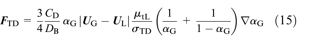
where
Wall lubrication force
To reduce gas volume fraction in near-wall region (distance of one bubble radius from the wall), a wall lubrication force is calculated according to Lubchenko et al., 6


where
Virtual mass force
The virtual mass force is calculated according to:

where virtual mass coefficient
Turbulence modelling
Turbulence is modelled only in the liquid phase, assuming that the flow of gas phase is laminar.
To model turbulent stresses in the liquid phase, Boussinesq eddy viscosity assumption is applied. It assumes that Reynolds stress tensor
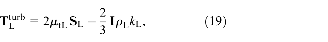
where
Based on the comparison of single-phase liquid turbulent vertical pipe flows (not shown in this paper) using different LRN models already implemented in OpenFOAM, Launder-Sharma
In this model, turbulent viscosity is given as:

where

where
Turbulent kinetic energy


where

Model constants have the values:

where
It should be noted that in Launder-Sharma model
Term
Bubble induced turbulence (BIT) closure modelling
Due to the presence of the bubbles and their interaction with the liquid phase, the profiles of liquid turbulent kinetic energy and liquid turbulent dissipation rate are modified compared to the case of pure liquid flow. To take into account this modification, source terms


where
Parameter
Summary of experimental data
To examine described numerical models for upward turbulent bubbly flow in a vertical pipe, comparisons of numerical simulation results against experimental databases for such flows are necessary. The selected databases are: Hosokawa and Tomiyama, 5 Liu 30 and Shawcat et al. 20 Main parameters of these experiments are listed in Table 1. The experimental test facilities used in these three cases are similar but still differ from each other. Therefore, not all of them are presented separately in this paper. They are graphically presented and described in detail in the mentioned papers. Also, more specific details about the measurement procedure and the measuring equipment used can be found there. A brief description of each experiment follows.
Summary of experimental sets: pipe diameter

Hosokawa and Tomiyama experimental database
In experiment of Hosokawa and Tomiyama,
5
the inner diameter of the vertical pipe was
The mixing section of air and water was at the bottom of the vertical pipe. Gas and liquid volumetric flows were measured by flowmeters before the mixing section. The liquid and gas volumetric fluxes
A laser Doppler velocimetry system (LDV, DANTEC, optics: 60 × 83, processor: 68N10) was used for measuring liquid velocities. Around 50,000 velocity data were taken for each measurement point. The uncertainty estimated at
Experiments were performed for four cases, in the present study referred as H1, H2, H3 and H4. This experimental database provides results of measurements of the relative velocity between gas and water
Liu experimental database
The results of an extensive set of experimental investigations of an upward two-phase bubble flow through the vertical pipe are presented in Liu. 30
The pipe was
For injecting air into the water flow, a bundle of
At the measuring station, both one-dimensional hot film sensor (TSI 1218-20W,
A dual-sensor resistivity probe was used for measuring the bubble velocity
Because of using hot-film anemometry, it was important to precisely control the water temperature. Water was cooled in the storage tank to achieve water temperature
From
Shawkat et al. experimental database
The ratio of pipe diameter and mean bubble diameter has a significant influence on the flow patterns and phase distribution.
20
Therefore, in contrast to Hosokawa and Tomiyama
5
and Liu,
30
who conducted two-phase bubbly flow experiments in vertical pipes of diameter
The pipe length was
For mixing of air and water, a showerhead injector was used. The injector had
During the experiments, the water temperature was kept within a range of
In this experimental database radial distributions of liquid velocity
Numerical simulation set-up
To perform numerical simulations of two-phase bubbly flow in a vertical pipe, solver twoPhaseEulerFoam of OpenFOAM v1906 is modified. These modifications include implementations of the following:
proposed relation for increase in the drag coefficient due to shear, given by equation (12)
lift force, equation (14)
wall lubrication force, equations (16) and (17)
BIT source terms, equations (26) and (27).
The computational domain, initial and boundary conditions and physical parameters of phases are explained in the continuation of this section.
Computational domain
Since in all analysed experiments the flow was assumed as axisymmetric, in order to reduce the number of computational cells, a quarter-pipe geometry is used in all simulations. The sketch of the computational domain is shown in Figure 2.

Sketch of a computational domain. A quarter-pipe is used in simulations.
The computational domain is bounded by five surfaces: inlet and outlet in the horizontal plane, pipe wall and two vertical symmetry planes.
Values of pipe diameters
The computational domain is discretised using O-grid block topology. This provides a high level of control of important mesh quality parameters like orthogonality, skewness and stretching of the cells. A typical example of this mesh in a pipe cross-section is shown in Figure 3. Mesh is generated using the blockMesh utility of OpenFOAM.

Computational mesh of a pipe cross section.
Since the LRN model is used, the value of non-dimensional distance
Mesh refinement study
Suitable discretisation of computational domain concerning the optimal number of cells is determined by grid sensitivity studies for each experimental database. Numerical calculations are performed on meshes with a different number of cells. Results are compared and optimal mesh is chosen.
As an example, a sensitivity study for one of the experiments of Hosokawa and Tomiyama 5 (case H1, see Table 1) is shown in Figure 4. Numerical calculations are performed on three meshes, named Mesh 1 (low refinement), Mesh 2 (medium refinement) and Mesh 3 (high refinement). The number of cells is presented in Table 2.
The mesh sensitivity test for case H1 (see Table 1) is performed on three meshes: Mesh 1 with 165,800 cells (), Mesh 2 with 320,000 cells (), and Mesh 3 with 409,400 cells (······). The results are shown for: (a) relative velocity, (b) void fraction and (c) liquid turbulent kinetic energy.
Cell numbers of meshes used in mesh sensitivity tests for cases H1, L1 and S1 (see Table 1).
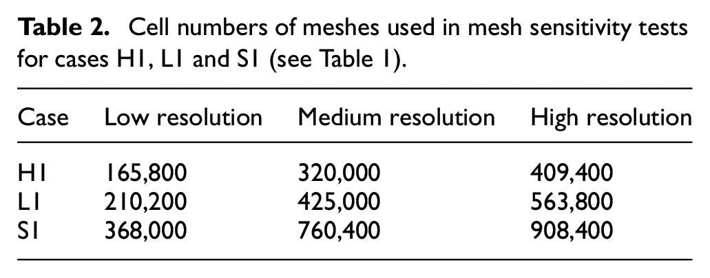
It is noticeable that the radial distribution of relative velocity and void fraction does not depend on the mesh density (Figure 4(a) and (b)). However, the kinetic energy profile (Figure 4(c)) obtained using Mesh 1 differs from the profile obtained using Mesh 2. No additional differences are found from the medium (Mesh 2) to the high refinement (Mesh 3) resolution.
It is concluded that the results obtained using Mesh 2 do not depend on the mesh density. Similar analyses were performed for each case listed in Table 1.
Table 2 provides data on meshes corresponding to cases H1, L1 and S1, of Hosokawa and Tomiyama, 5 Liu 30 and Shawkat et al., 20 respectively (see Table 1). Meshes with medium refinement are found as optimal computational meshes.
Initial and boundary conditions
Uniform phase velocities are set as the boundary condition at the inlet surface. These velocities are calculated as the ratio of phase volumetric fluxes and the corresponding phase volume fraction,
At the outlet surface, a zero-gradient boundary condition is defined for
At the pipe wall, a no-slip boundary condition is applied for both phase velocities and fixed zero value for the void fraction. For turbulent kinetic energy and dissipation zero values are prescribed at wall (actually, values of
Initial conditions inside the computational domain for all quantities are identical to their values in the inlet section.
Physical parameters of phases
Liquid flow is calculated as incompressible. Gas is treated as an ideal gas. Phase densities, phase viscosities and surface tension are prescribed based on their values at atmospheric pressure and temperatures from experiments.
Mean void fraction and mean bubble diameter are defined in papers of Hosokawa and Tomiyama 5 and Liu, 30 while for experimental case of Shawkat et al. 20 these quantities are calculated by integration of experimental results:

Numerical simulations are conducted with constant mean bubble diameter. Spherical bubbles are assumed.
Volumetric fluxes of gas and liquid, mean bubble diameters and void fractions for experimental cases examined are specified in Table 1.
Solution method
The pseudo-steady state solution is obtained using PIMPLE algorithm for pressure-velocity coupling. Time step size is set up to be adaptive, based on the condition of maximum Courant number equal to
Spatial and time discretisation schemes are of the second order.
Results and discussion
In order to determine the effects of the new proposed correlation for the drag coefficient of a single bubble in a shear flow, given by equation (12), the results of numerical simulations conducted with this new correlation are compared to the results of numerical simulations conducted with the drag coefficient for a single bubble in a uniform stream, given by equation (5). The remaining conditions for these simulations are the same, as described in previous sections. Results of both numerical simulations are tested against the experimental data of Hosokawa and Tomiyama, 5 Liu 30 and Shawcat et al. 20
Hosokawa and Tomiyama
The first column of Figure 5 shows radial profiles of relative velocity calculated in numerical simulations along with experimental data of Hosokawa and Tomiyama. 5
Radial distribution of relative velocity ) experimental data from Hosokawa and Tomiyama
5
; () numerical predictions when drag coefficient is calculated for a single bubble in a uniform stream, equation (5); () numerical predictions with included new correlation for the drag coefficient, equation (12). The first three diagrams (a), (b) and (c) represents case H1, the diagrams (d), (e) and (f) represents case H2, the diagrams (g), (h) and (i) case H3 and last three diagrams (j), (k) and (l) represents case H4.
Numerical simulations with a drag coefficient for a single bubble in a uniform stream, given by equation (5), for all cases examined (H1, H2, H3 and H4) predict uniform relative velocity up to
In contrast, if the drag coefficient is calculated for a single bubble in a shear flow, given by equation (12), numerical simulation results for relative velocity compare very well against corresponding experimental results, for all cases examined (Figure 5(a), (d), (g) and (j)). With the increase of liquid volumetric flux (for the same pipe diameter), there is an increase in the liquid shear rate. That further increases the drag coefficient of a single bubble (see equation (12)) and reduces the relative velocity, assuming that the drag force on a bubble is constant. This explanation is in accordance with experimental data: a stronger relative velocity reduction is observed for cases H3 and H4 (Figure 5(g) and (j), respectively) with higher liquid volumetric fluxes compared to cases H1 and H2 (Figure 5(a) and (d), respectively), with lower liquid volumetric fluxes.
This shows that in this particular case, under all the above conditions of two-phase bubbly flow, it is necessary to take into account the influence of shear flow on the drag coefficient (described by the new equation (12)) in order to correctly predict the relative velocity profile.
Radial distributions of void fractions obtained from numerical simulations and experimental results of Hosokawa and Tomiyama
5
are shown in the second column of Figure 5. According to experimental data, all cases examined have pronounced wall-peak void fraction profiles, except case H2 (Figure 5(e)) that has an approximately uniform void fraction up to
The third column in Figure 5 represents the radial distribution of liquid turbulent kinetic energy obtained from numerical simulations and experimental data of Hosokawa and Tomiyama.
5
The overall agreement between experimental and numerical simulation results is good. For smaller liquid volumetric flux, cases H1 and H2 (Figure 5(c) and (f), respectively) there is a small underprediction of numerical simulation results for
Considering that results of numerical simulations conducted with drag coefficient for a single bubble in uniform stream, equation (5), almost coincide with results of numerical simulations conducted with drag coefficient for a single bubble in shear flow equation (12), it can be concluded that an increase in the drag coefficient due to shear flow does not affect liquid turbulent kinetic energy.
According to the case of Hosokawa and Tomiyama, 5 it can be concluded that the biggest influence of a drag coefficient of a single bubble in a shear flow (compared to a drag coefficient of a single bubble in a uniform stream) is achieved on the relative velocity of air and water. This conclusion is checked when the flow occurs in pipes of larger diameter in experiments of Liu 30 and Shawkat et al. 20
Liu
In contrast to the experimental database of Hosokawa and Tomiyama 5 where relative velocities of phases are given, in the experimental database of Liu 30 both air and water velocity profiles for all experiments are available. Therefore, the influence of the drag coefficient of bubbles, given by equations (5) and (12), on both the liquid and gas phase, can be analysed separately.
Liquid velocity profiles from numerical simulations and experimental database of Liu
30
are plotted in the first row of Figure 6. It can be seen that there is an excellent agreement of numerical simulation results conducted with a drag coefficient for a single bubble in a uniform flow, given by equation (5) and results of numerical simulations conducted with a drag coefficient for a single bubble in the shear flow, given by equation (12). The reason for this behaviour is that due to small values of mean void fractions
Radial distribution of liquid phase velocity ) experimental data from Liu
30
; () numerical predictions when drag coefficient is calculated for a single bubble in a uniform stream, equation (5); () numerical predictions with included new correlation for the drag coefficient, equation (12). The diagrams in the first column (a), (d), (g) and (j) represents case L1, the diagrams (b), (e), (h) and (k) represents case L15, and the diagrams (c), (f), (i) and (l) represents case L29.
For case L1 shown in Figure 6(a), liquid velocity profile from experimental data agree very well with liquid velocity profile calculated in a numerical simulation. However, for case L15, shown in Figure 6(b), there is a small overprediction of numerical simulation results for
Regarding gas velocity profiles, for cases L1, L15 and L29, shown in Figure 6(d) to (f), respectively, results of numerical simulations conducted with a drag coefficient for a single bubble in the uniform stream, equation (5), agree very well with results of numerical simulations conducted with a drag coefficient for a single bubble in the shear flow, equation (12). For all cases examined, only a small difference between these results is visible for
For case L1 (Figure 6(d)), the gas velocity profile obtained from numerical simulations is slightly overpredicted for
Unlike the water velocity profile, the air velocity profile shows the dependence on the choice of the drag coefficient modelling. Taking into account the influence of shear flow on the drag coefficient has an impact on the air velocity profile, but in this case, it is small.
For cases L1, L15 and L29, it can be seen that profiles of void fraction (shown in Figure 6(g)–(i)), as well as profiles of liquid turbulent kinetic energy (shown in Figure 6(j)–(l)), obtained from numerical simulations conducted with a drag coefficient for a single bubble in a uniform stream agree very well with corresponding numerical simulation results performed with a drag coefficient for a single bubble in a shear flow.
For case L1, (Figure 6(g)), the agreement of radial void fraction calculated in the numerical simulation and experimental results is moderately good. However, with the increase of liquid volumetric flux, cases L15 and L29 (shown in Figure 6(h) and (i), respectively), numerical simulation results of void fraction become larger than the corresponding experimental values for
Experimental data of the radial distribution of liquid turbulent kinetic energy for case L1, shown in Figure 6(j), are slightly larger and more uniform across the cross-section than the results of liquid turbulent kinetic energy obtained from numerical simulations. For case L15, shown in Figure 6(k), the agreement of experimental results of liquid turbulent kinetic energy and corresponding results of numerical simulations is moderately good. However, further increase in liquid volumetric flux increases discrepancies between experimental and numerical simulation results, which is seen in Figure 6(l). As discussed in the results of Hosokawa and Tomiyama, 5 the reason for this discrepancy could be in the interfacial force models and/or in BIT models. Also, in numerical simulations monodisperse approximation has been used.
Shawcat et al
The first column of Figure 7 shows the liquid velocity profiles from the experiment of Shawcat et al.
20
and corresponding liquid velocity profiles calculated in numerical simulations. In these figures, there is no difference in liquid velocity profiles if numerical simulations are conducted with the drag coefficient for a single bubble in a uniform stream (equation (5)) or with a drag coefficient for a single bubble in a shear flow (equation (12). The reason for this is that due to small values of mean void fractions
Radial distribution of liquid phase velocity ) experimental data from Shawkat et al.
20
; () numerical predictions when drag coefficient is calculated for a single bubble in a uniform stream, equation (5); () numerical predictions with included new correlation for the drag coefficient, equation (12). The diagrams (a), (b) and (c) represents the results for case S1, while the diagrams (d), (e) and (f) represents the results for case S2.
Experimental results show that liquid velocity distribution is approximately uniform for
The second column of Figure 7 shows the radial distribution of air velocity. It is seen that air velocity profiles obtained in numerical calculations with a drag coefficient for a single bubble in the uniform flow, equation (5), and with a drag coefficient for a single bubble in the shear flow equation (12) are almost identical. The pipe diameter used in Shawkat et al.
20
is
Results of numerical computations overpredict liquid velocity in almost the entire cross-section, shown in Figure 7(a) and (d). In contrast, numerical computations predict slightly lower air velocities relative to the experimentally measured values, shown in Figure 7(b) and (e).
The third column of Figure 7 shows the radial distribution of the void fraction from experimental results and void fraction calculated in numerical simulations. Experimental results for the void fraction show an approximately uniform radial distribution with a small peak at
Besides imperfections in interfacial forces and/or in BIT models, as well as due to monodisperse approximation used in numerical simulations, an additional source for disagreement between experimental and numerical results in Figure 7 could be the difference between liquid and gas volumetric fluxes obtained from flowmeters and by integration of experimental measurements obtained using optical and hot-film probes in the measurement section. These differences for cases of Shawkat et al.
20
go up to around
Conclusions
Upward turbulent bubbly flows in vertical pipes are studied in the Euler-Euler framework of OpenFOAM. In almost all previous numerical studies of these flows available in the literature, high-Reynolds-number (HRN) models were used. In this paper, the turbulent bubbly flow is analysed using the low-Reynolds-number (LRN)
To account for the increase in the drag coefficient of a single bubble due to shear (compared to drag coefficient of a single bubble in uniform flow), a relation of Legendre and Magnaudet 21 is examined. It is found that the drag coefficient defined by Legendre and Magnaudet, 21 equation (10), goes to infinity towards the pipe wall, with an increase especially pronounced in cells near the pipe wall. That causes numerical instabilities and therefore this correlation is not applicable with LRN models.
To consider the increase in the drag coefficient of a single bubble due to shear, but to provide stability of numerical simulations performed with LRN models, a new correlation for the drag coefficient (equation (12)) is proposed. The new correlation is based on linear regression with experimental data of Hosokawa and Tomiyama. 5
To examine the effects of the proposed correlation for the drag coefficient for a single bubble in a shear flow (equation (12)), the results of numerical simulations conducted with it are compared to the results of numerical simulations conducted with the drag coefficient for a single bubble in a uniform stream (equation (5)). The remaining conditions for these two types of simulations are the same. Besides the drag force, other interfacial forces taken into account by these numerical simulations are: lift force of Shaver and Podowski, 25 turbulent dispersion force of Burns et al., 26 wall lubrication force of Lubchenko et al. 6 and virtual mass force. The bubble induced turbulence model of Colombo and Fairweather 29 is used in numerical simulations.
The numerical simulation results are compared against experimental databases of Hosokawa and Tomiyama, 5 Liu 30 and Shawkat et al. 20
A comparison of numerical simulation results with all three experimental databases shows that the choice of correlation for calculating the drag coefficient, whether it takes into account the influence of shear flow (equation (12)) or not (equation (5)), has no significant effect on the profiles of liquid turbulent kinetic energy
The biggest influence of the increase of the drag coefficient of a single bubble in shear flow (equation (12)), compared to the drag coefficient of a single bubble in uniform flow (equation (5)), is achieved on the relative velocity of air and water, in the case of Hosokawa and Tomiyama. 5 In this case, without implementing a new correlation for the drag coefficient, equation (12), numerical simulations cannot correctly predict the relative velocity profile.
In the case of Hosokawa and Tomiyama 5 relative velocity profiles are available, while in the other two cases of Liu 30 and Shawkat et al., 20 velocity profiles of both phases are presented.
Analysing the results of Liu, 30 it is concluded that the air velocity profile depends on the correlation choice for the drag coefficient (equation (5) or equation (12)), while this choice does not affect the water velocity profile.
As expected, in the case of Shawkat et al. 20 the water velocity profiles do not depend on whether equation (5) or equation (12) is used in the calculation. However, in this case, the air velocity profile also does not depend on the drag coefficient modelling. As discussed in the previous chapter, the influence of the new correlation equation (12) on the air velocity profile decreases as the liquid velocity gradient decreases. This is often the case in larger diameter pipes.
Based on all the above, it is recommended to use a new correlation for the drag coefficient equation (12) which considers the influence of shear flow and which is compatible with LRN models. For flows through pipes of relatively small diameter (e.g. Hosokawa and Tomiyama 5 and Liu 30 ), the velocity gradient has higher values. In such cases, the use of equation (12) will lead to a better prediction of the air velocity profile (and thus the relative velocity profile). When the flow takes place in pipes of larger diameter (e.g. Shawkat et al. 20 ), the velocity gradient usually has smaller values, so the equation (12) will not lead to a change in the calculation results.
In all calculations, velocity profiles are predicted with satisfactory accuracy. In some places, there are larger deviations in the
The numerical solver created in this study is freely available at the Github: https://github.com/darkoradenkovic/EulerEulerSimulationsInOpenFoam.git.
The developed solver can further be used in the development of more advanced wall functions in the context of turbulent wall-bounded bubbly flows or in turbulent bubbly flow studies where fine resolution of flow quantities is necessary.
Footnotes
Handling Editor: Chenhui Liang
Declaration of conflicting interests
The author(s) declared no potential conflicts of interest with respect to the research, authorship, and/or publication of this article.
Funding
The author(s) disclosed receipt of the following financial support for the research, authorship, and/or publication of this article: This work is financially supported by the Ministry of Education, Science and Technological Development Republic of Serbia (MESTD), contract number 451-03-68/2020-14/200105 (subproject TR35046).