Sage Journals: Discover world-class research

Abstract

In pavement design, vehicle load is typically simplified as vertical circular uniform loading. Due to the vehicle dynamic effect and deformation of a tire, non-uniform three-dimensional contact stresses are produced at the contact interface between the tire and pavement under different driving modes. For this paper, an 11R22.5 truck radial tire was selected. Considering the geometric nonlinearity and large deformation of the tire and nonlinear characteristics of tire-pavement contact, the Neo-Hookean and Rebar models are used to simulate the hyperelastic rubber material and rubber-cord composite material, respectively. The three-dimensional contact stress distribution under static, free rolling, acceleration, braking, and cornering modes was simulated and analyzed. The results show that inflation pressure, axle load, and friction coefficient of the tire significantly affect the three-dimensional contact stress distribution. Further, three-dimensional stresses are non-uniformly distributed, rather than in the traditional simplified circular uniform load. The three-dimensional stress distribution of tire-pavement in different driving modes is also significantly different. The vertical and lateral stresses in the state of cornering are the largest, the longitudinal stress in the state of braking is the largest as well. The research results provide reference for future pavement design and pavement damage analysis.

Keywords

Highway engineering radial tire finite element tire-pavement contact three-dimensional contact stress acceleration braking cornering

Introduction

Due to the vehicle dynamic effect, rolling friction and sliding friction between tire and pavement, and the deformation of a tire, when a vehicle is in normal driving, that is, acceleration, braking and cornering, non-uniform three-dimensional contact stresses are produced at the tire-pavement contact interface. At present, vehicle load is assumed to be static vertical circular uniform loading in asphalt pavement structure design methods, and the contact stress and tire inflation pressure are equal. However, vertical uniform load and non-uniform three-dimensional contact stresses will lead to different structural responses^1–3in asphalt pavement. For example, many researchers believe that Top-down cracking^4–6 and road surface rutting⁷ of asphalt pavement are related to non-uniform three-dimensional stresses at the tire-pavement contact interface.

Two methods are used to obtain the tire-pavement contact stress distribution: field measurement and theoretical analysis. Field measurement methods such as De Beer et al.^8,9 use the Vehicle-Road Surface Pressure Transducer Array (VRSPTA) to measure the three-dimensional contact stresses, however, this method is time-consuming and expensive, and the accuracy of the results depends on sensor resolution, the friction performance between the pavement surface and the tire, and the number of sensor arrangements.

Meanwhile, the development of numerical analysis and calculation technology makes theoretical analysis methods feasible. Some studies have established tire models by a finite element method to predict tire-pavement contact stress or evaluate tire performance. For example, Tielking and Roberts¹⁰ established the finite element model of the bias-ply tire, assuming that the pavement is a rigid body, analyzed the influence of tire pressure and load on the contact stress and found that structural strain generated by non-uniform contact stresses is significantly higher than that generated by a uniform load. Zamzamzadeh and Negarestani¹¹ established a finite element model of a 205/60 R14 radial tire by ABAQUS, in which rubber materials were compared with different elastic models, the purpose was to evaluate the behavior of the rolling tire when contacting with pavement and to optimize tire performance. Zhang¹² developed a non-linear finite element model for a radial truck tire using FEM based to analyze the various stress fields with a particular focus on inter-ply shear stresses in the belt and carcass layers, the author derived a more desirable set of structural parameters that could lead to lower values of maximum shear stresses within the loaded multi-layered tire structure. Meng¹³established a 295/75 R22.5 Low-Profile Radial smooth tire model on rigid pavement and analyzed vertical stress under different load conditions, the Coulomb friction law was used to study the contact between the truck tire and pavements. The results showed that the average stress used in the AASHTO seriously underestimates the maximum stresses served by pavements, with the result that a highway could be seriously under designed. Wang and Roque¹⁴ and Al-Qadi and Wang¹⁵ established three-dimensional finite element modeling of tire-pavement interaction, they analyzed the three-dimensional contact stress distribution and pavement structural response. The results showed that the possibilities of longitudinal fatigue cracking, primary rutting, and secondary rutting in thin asphalt pavement were increased. The heavy loading caused increasing responses in the base layer and subgrade, while high tire inflation pressure caused an increasing response in the asphalt mixture layer, especially for the shear stress at high temperature. However, the authors only considered the static state of a tire. Wang and Al-Qadi¹⁶ also considered the influence of a tire static state and different rolling states on three-dimensional stress. The results showed that the non-uniformity of vertical contact stresses decreasing as the load increases but increasing as the inflation pressure increases. Vehicle maneuvering behavior significantly affected the tire-pavement contact stress distributions. Zhou et al.¹⁷ simulated the effects of different friction models on tire braking. A truck radial tire (295/80R22.5) was modeled, and an exponential decay friction model that considers the effect of sliding velocity on friction coefficients was adopted for analyzing braking performance. It is found that the change of driving conditions has a direct influence on tire-pavement contact stress distribution. The results provide the guidance for tire braking performance evaluation.

The above studies provide a good reference for the work in this paper. In order to better analyze the stress-strain response of the pavement structure under the non-uniform contact stress conditions, the tire-pavement contact stress distribution and its magnitude for different tire inflation pressures, different tire loads, different friction coefficients and different driving conditions such as acceleration, deceleration and cornering need to be analyzed.

The primary objective of this paper is to establish a three-dimensional tire model and a tire-pavement contact model with the 11R22.5 radial tire commonly used by trucks in China as the research object by using the finite element method. The three-dimensional contact stresses distribution under static, acceleration, braking, and cornering conditions are simulated and analyzed.

The objective involved the following tasks:

Based on the parameters of tire manufacturers, a three-dimensional model of a tire is developed based on geometric structure and tire size.

Develop a three-dimensional FEM-based model of the tire–pavement interaction.

Use the model to predict contact stresses of tire–pavement interface for multiple inflation pressures and axle loads, including different friction coefficients.

Use the model to predict three-dimensional stresses distribution at tire-pavement interface by simulating tires during free rolling, acceleration, braking, and cornering.

Finite element modeling of a radial tire

Tire types and parameters

Tires can be classified as bias-ply tires and radial-ply tires owing to the different arrangements of cords. A radial tire is composed of six main parts: tread, carcass, sidewall, braker ply (or belt layer), bead, and inside layer (or air-tightness layer). In order to bear the large tangential force when a vehicle is traveling, the cord of a carcass is arranged in a radial direction. The multi-layered belt cords are positioned at opposite angles with respect to the center line of the tread, ranging from 10° to 20°. The cord is made of steel wire or fabric using materials with high rigidity, high strength, and small deformation, such as artificial silk and nylon.

For this paper, a 11R22.5 radial tire is selected. In the tire specifications, “R” denotes radial construction, while “11” and “22.5” stand for tire cross-section width and wheel hub diameter, respectively, in inches. The parameters are shown in Table 1.

Table 1.

Parameters of 11R22.5 tire.

Inflation pressure	Maximum axle load(single/dual)	Load Index(single/dual)	Width ofcross-section	External diameter	Rollingcircumference	Minimum dualspacing
0.72 MPa	2800 kg/2650 kg	144/142	279 mm	1065 mm	3344 mm	318 mm

On the plane parallel to the pavement surface, the longitudinal (x direction) is along the vehicle driving direction, the lateral is transverse to the vehicle driving direction (y direction). In addition, the vertical is vertical in the pavement surface direction (z direction), as shown in Figure 1.

Figure 1.

Tire sign convention.¹⁴

Tire material partition composition

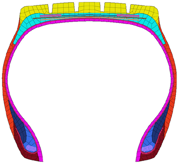
An 11R22.5 truck radial tire is composed of different rubber and cord materials. Among them, the rubber material is divided into seven parts: Tread rubber, BeltSKM (belt layer rubber), Innerliner (inside layer rubber), Side (sidewall rubber), Rimcout, BeadFL1 (upper triangular rubber) and BeadFL2 (lower triangular rubber). The cord materials are divided into six parts: Belt1, Belt2, Belt3, Belt4, Ply, and Bead. As shown in Figure 2, different colors represent different material regions.

Figure 2.

Material partition of 11R22.5 tire.

Tire model

Due to the complexity of tire structure and composition materials, it is difficult to accurately construct a tire model. ABAQUS software can analyze the rolling behavior of a tire under steady and transient conditions, and solve the nonlinear problem by a complete Lagrange method. In this paper, the tire is regarded as a composite structure composed of a hyperelastic rubber material and a high strength cord ply layer with steel wire belt. Considering the geometric nonlinearity and large deformation of tire and the nonlinear characteristics of tire-pavement contact, the tire-pavement contact model was established by ABAQUS with the boundary condition setting, and obtaining its nonlinear solution.

Tire rubber material model and parameters

Rubber material of the tire is non-linear incompressible or approximately incompressible hyperelastic material.¹⁸ It will produce a large deformation under loading, but it can still recover after unloading, so its constitutive relationship is complex. Simulation of hyperelastic materials requires the following assumptions: the material is elastic, isotropic, and incompressible,¹⁹ further, geometric nonlinear effects need to be considered in a simulation.

A hyperelastic constitutive model of rubber materials can be divided into two categories: a phenomenological model based on a continuous medium, and statistical model based on thermodynamics.²⁰ The continuum model is described by the internal strain energy of rubber materials, rather than being characterized on the basis of the polymer molecular structure. The core point is to establish the expression of system’s storage elastic energy.²¹ There are two forms of a phenomenological model based on the continuous medium theory, one is a hyperelastic constitutive model that uses strain invariants I₁, I₂, and I₃ to characterize strain energy (E), such as the Mooney-Rivlin model, Yeoh model, Neo- Hookean model, etc. Among them, the Neo-Hookean model is suitable for small and medium deformations, and the Yeoh model is used for large deformation situations. The other is a continuum model based on elongation, where its strain energy function can be characterized by the main elongation. Such models include: the Ogden model, Shariff model, Attard model, etc.²²

The Neo-Hookean model is more accurate in simulating the tensile, compressive, and pure shear behavior of rubber materials.²³ The Neo- Hookean model based on the continuum phenomenological model is used in this paper to simulate tire rubber materials. Its strain energy function expression is:

U = C_{10} ({\bar{I}}_{1} - 3) + \frac{1}{D_{1}} (J_{el} - 1)^{2}

(1)

In the equation, U represents strain potential energy, $C_{10}$ represents the shear characteristics of the material, $J_{el}$ is the elastic volume ratio, ${\bar{I}}_{1}$ represents the deformation of the material, and $D_{1}$ represents the compression characteristics of the material.

The tire industry does not make exact material properties and structural design of tires available to the general public. At the same time, the workload and cost of testing for tire materials are relatively large. Therefore, the model parameters of rubber materials in Cui²⁴ are used, as shown in Table 2.

Table 2.

Rubber material parameters of 11R22.5 tire.

Materials	$C_{10}$	$D_{1}$	ρ(g/cm³)
Tread	1.000	0.0198	1.1
BeltSKM	1.139	0.0240	1.1
Innerliner	0.953	0.0300	1.1
Side	1.000	0.0600	1.1
Rimcout	1.406	0.0200	1.1
BeadFL1	1.606	0.0200	1.1
BeadFL2	0.671	0.0300	1.1

Tire cord ply model

Cord ply materials are formed by the arrangement of cords as reinforcement in the rubber, having obvious anisotropic properties. The common model mainly includes a Layer-Shell model and Rebar model. Since the parameters of a Layer-Shell model are obtained from experiments, it is difficult to obtain.²⁵ However, by dividing the cord ply into two independent parts, the Rebar model is established by combining the rubber model and cord material model based on the actual composition of the tire, thus, the model better reflects actual structure of the tire. The Rebar model is used in the paper, the parameters²⁴ are shown in Table 3.

Table 3.

Cord-rubber material model parameters of 11R22.5 tire.

Structure regions	E (Pa)	Poisson’s ratio	ρ(g/cm³)
Belt1	1.14e+5	0.4	7.50
Belt2	1.14e+5	0.4	7.50
Belt3	8.40e+4	0.4	3.95
Belt4	8.40e+4	0.4	7.50
Ply	1.50e+4	0.4	2.00
Bead	2.00e+5	0.3	7.80

Establishment of tire model

Two-dimensional tire model and meshing

The two-dimensional tire model is the one plane surface of the three-dimensional model, and the three-dimensional model can be generated by revolving around the axis of symmetry. First, a two-dimensional tire model is established. According to the two-dimensional AutoCAD cross-sectional view of the tire, the graphic file is output in an Iges format file, which can be converted into a two-dimensional plane view that can then be imported into HyperMesh software, thus, a two-dimensional finite element model of the tire can be established.

The meshing of the model plays a vital role in the results of the finite element analysis and will directly affect the calculation time, accuracy, and convergence of the results. In order to ensure the accuracy of the finite element simulation, the tire model is strictly divided into elements according to the material boundary, and the triangular element is only used at the sharp corners of the material boundary, and quadrilateral elements are used for other sites. In addition, the elements are appropriately detailed in the location of stress concentration, such as at the bead or the belt end area where the stress-strain gradient is larger.

Meshing is done with HyperMesh software, which, compared with the traditional method in ABAQUS, improves upon mesh quality and modeling accuracy. The CGAX4H element is used in a two-dimensional axisymmetric model, and its corresponding three-dimensional model element is C3D8H. The CGAX3H triangular element is used for a two-dimensional model, its corresponding three-dimensional model element is C3D6H. A three-dimensional four-node element SFM3D4 can be obtained by revolving the linear element SFMGAX1 of the Rebar model.

Because the tire section is axisymmetric, it is only necessary to mesh the left half of the tire, obtain the right half of the mesh by using the mirror copy function, and connect the adjacent nodes of the left and right parts of the mesh to obtain a complete two-dimensional tire model, as shown in Figure 3. The total number of two-dimensional model nodes is 704, the number of element is 579, the total number of rubber element is 368, including 344 quadrilateral elements, 24 triangular elements, and 211 Rebar linear elements.

Figure 3.

Two-dimensional tire model meshing.

In order to analyze the ground connection situation of the tire, the tire needs to be inflated before loading. The method is to apply a uniformly distributed load on the tire’s inner surface, and the direction of the load is perpendicular to the inner surface of the tire. According to Size designation, dimensions, inflation pressure, and load capacity for trucktires,²⁶ the standard inflation pressure of a heavy-duty radial tire 11R22.5 is 0.72 MPa, and the pneumatic tire model is shown in Figure 4.

Figure 4.

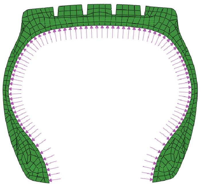
The inflation of tire.

Modeling and assembly of rim

The traditional method models the wheel hub separately then assembles the tire and the wheel hub. It is necessary to set the contact pair between the rigid and the deformable bodies during assembly process, it is also necessary to ensure there is no overlap between the tire model and the wheel hub model, that is, no penetration constraint.

Referring to the existing research,^23,27 the above problems are simplified reasonably in this paper, that is, the tire-rim contact is used to treat the rim as a rigid body, and the fixed constraint is used on the sidewall at the part of the tire-rim contact to limit the degrees of freedom in three directions. Thus, in rim modeling, the sidewall is defined as a rigid element by omitting the wheel hub.

The rim edge is simulated as a rigid structure, which is closely connected to the tire bead and axle, thus, it is not necessary to consider the rim assembly. The rigid structure reference point is located on the axis, and boundary conditions are specified at this node to allow the structure to rotate around the axis. Compared with the traditional method, it better solves the problem of contact nonlinearity and improves accuracy of calculation. At the same time, Lagrange rolling analysis must be performed in the simulation, which requires higher mesh quality of the tire surface and indicates that this method is feasible. The established tire-rim assembly model is shown in Figure 5.

Figure 5.

Tire-rim assembly model.

Generation of 3D model of wheel assembly

After thetwo-dimensional tire model is inflated, a complete three-dimensional finite element model can be generated by revolving the 2D finite element model by symmetric model generation technique.

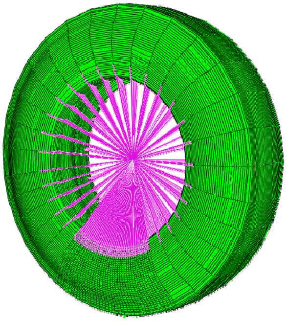
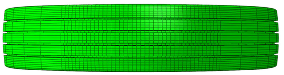
In order to create the three-dimensional model more accurate and improve the calculation efficiency via minimizing the number of elements while revolving, when generating the three-dimensional model, we specify the bottom 60° area as the contact area between the tire and the pavement, which is divided into 40 discrete segments, where the two 50° areas on both sides of the bottom are divided into five discrete segments, and the remaining 200° area is divided into 16 discrete segments, as shown in Figure 6. The final three-dimensional tire model is shown in Figure 7, the three-dimensional model of each tire’s component is shown in Figure 8.

Figure 6.

The discrete segment of the wheel.

Figure 7.

The three-dimensional model of the wheel.

Figure 8.

The three-dimensional model of each component of the wheel.

Tire-pavement contact model

To ensure quality of the element and improve accuracy of simulation analysis, some tire sites are simplified, namely: omitting the tread lateral pattern and using four longitudinal groove patterns instead, and simplifying the detailed geometric information such as tire anti-friction lines and marking lines. When modeling, the longitudinal pattern and tread are classified as the same material area, as shown in Figure 9.

Figure 9.

Longitudinal groove patterns of tire.

The tire will be deformed when subjected to force, however, the tire deformation is much larger than the pavement deflection. Results of an earlier study indicated that tire–pavement interface stresses are independent of pavement structural characteristics. Therefore, in order to ensure the convergence of the calculation results and efficiency, according to the literature,¹⁰ it assumed that the pavement structure has no deformation. At the same time, the contact pair is defined to simulate the contact between the tire and the pavement, and the friction coefficient is used to simulate the interactive relationship between the tire and the pavement. According to the literature,²⁸ the friction coefficient is 0.5. The tire-pavement contact model is shown in Figure 10.

Figure 10.

The three-dimensional contact model between the tire and the pavement.

In order to ensure accuracy of the simulation, it is necessary to verify whether the tire model is correct and reasonable. Due to condition limitations, it is difficult to verify by testing the mechanical properties of tires. The usual method is to test the sensitivity of the tire’s macroscopic dimensions variation under loading. The indicators that can reflect the sensitivity of tire model include tire diameter, section width, deflection etc. The test data of the Test Center of Shanghai Tire & Rubber (Group) Co., Ltd. Tire Research Institute provided by the literature²⁹ are adopted in this paper, a comparison between the model simulation results and the measured results is shown in Table 4, where the load is 25 kN. The comparison shows that the error of load-deflection and load-section width are both less than 4%, indicating that the tire finite element simulation results are in good agreement with the measured results, where the load-deflection refers to the deformation of the center of rim mass downward under loading.

Table 4.

Comparison of simulation and measured results (Load: 25 kN).

Items	Simulationresults	Measuredresults	Error (%)
Load-deflection(mm)	34.36	35.6	3.48
Load-sectionwidth (mm)	307.12	313.0	1.88

Results and discussions

Static contact analysis

The tire-pavement contact analysis under static conditions can be simulated in two steps. First, apply inflation pressure to the inner surface of the tire model and set different inflation pressure levels to meet the analysis requirements. Second, the vertical axle load is gradually applied to the rim shaft under a given inflation pressure and a specified time step. In order to study the relationship between tire-pavement surface contact stress and tire inflation pressure and load, the given inflation pressure is set at 0.62, 0.67, 0.72, 0.77, and 0.82 MPa respectively, the single tire load is set to 22, 25, 28, 31, and 34 kN.

Effect of inflation pressure

The single tire load is 28 kN, the three-dimensional contact stress under five different inflation pressures is shown in Figure 11, the friction coefficient is 0.5 for analysis, locations of peak contact stresses are shown in Figure 12.

Figure 11.

Three-dimensional contact stress nephogram under different inflation pressures.

Figure 12.

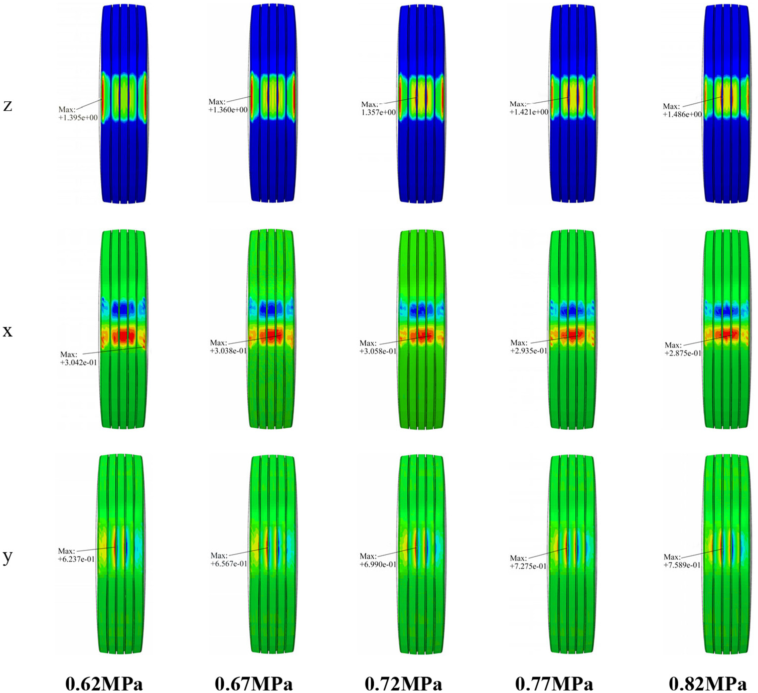
The locations of three-dimensional peak contact stresses under different inflation pressures.

In Figure 11, z represents vertical, x represents longitudinal, and y represents lateral. They are also the same meanings in Figures 12 to 16.

Figure 13.

Three-dimensional contact stress nephogram under different loads.

Figure 14.

The locations of three-dimensional peak contact stresses under different loads.

Figure 15.

Three-dimensional contact stress nephogram under different friction coefficients.

Figure 16.

The locations of three-dimensional peak contact stresses under different friction coefficients.

It can be drawn from Figures 11 and 12:

The tire-pavement surface contact area is approximately rectangular instead of a traditional circular shape, the three-dimensional stress is non-uniform distributed on the contact surface.

When the inflation pressure is low, the maximum vertical stress distributes at the outer edge of the tire. With an increase of inflation pressure, the maximum vertical stress shows a trend, which is that it first becomes smaller and then gradually increases, the position is from edge transfer to the center of the wheel track.

This is because the lower the inflation pressure, the greater the sinkage of the tire, then the tire grounding area increases, thus, the stress distribution of the grounding area becomes low in the middle area and high at the tire edge, that is, the phenomenon of warpage of the tire occurred, so the pressure at the tire edge is the largest, the tire center area is smaller. As the inflation pressure increases, the tire contact area decreases, the stress at the edge of the tire gradually decreases, and the stress at the center area of the tire gradually increases. This is also consistent with the findings in the literature.^23,30

In addition, during the process of tire inflation, due to tire construction, first, the tire shoulder is more strongly in contact with the pavement, followed by transferring to the tire tread and the pavement contact gently, and, finally transferring to the tire center area tread and the pavement contact more strongly, which resulted in the changing of contact area from small to large and then smaller during this period. Therefore, the maximum vertical stress should first become small and then increase.

Maximum longitudinal and lateral stresses are not located at the center of the tire.

With increasing inflation pressure, the longitudinal contact stress in general shows a decreasing trend, such as when the inflation pressure increases from 0.62 to 0.82 MPa, the maximum longitudinal stress decreases from 3.402e-01 to 2.875e-01, while the lateral stress gradually increases, which agrees with the measurements and results of other studies.¹⁴

Longitudinal and lateral stress are antisymmetric distributed at the tire lateral center and longitudinal center, respectively, as such, the sum of longitudinal and lateral stress on the entire contact surface is zero. However, there are still longitudinal and lateral stresses in different areas of the tire-pavement surface contact surface, and their influence on the response of the pavement structure cannot be ignored.

Effect of load

The inflation pressure is 0.72 MPa, three-dimensional contact stress under five different single tire loads is shown in Figure 13, the friction coefficient is 0.5 for analysis, locations of peak contact stresses are shown in Figure 14.

It can be drawn from Figures 13 and 14:

The tire-pavement surface contact area is approximately rectangular; the three-dimensional stress is non-uniform distributed.

When the load is small, the maximum vertical stress is located at the center of the tire. As the load increases, its position gradually shifts from the center of the tire to the edge of the tire. This finding agrees with measurement results and other studies.^8,31 The results show that a heavy load causes greater bending deformation of the tire sidewall, and the compression of the tire sidewall by the pavement surface is stronger than the compression of the tire center.

With the load increase, the maximum vertical stress values increase gradually, such as when the load increases from 22 to 34 kN, the maximum vertical stress increases from 1.366e-01 to 1.682e-01, the load growth rate is 54.5%, while the vertical stress growth rate is 23%, the stress growth rate is less than that of load. This indicates that, as the load increases, the tire contact area also increases, resulting in smaller growth of vertical stress.

The maximum longitudinal and lateral stresses are not located at the center of the tire.

As the load increases, the longitudinal stress gradually increases, while the lateral stress gradually decreases. This means that as the load increases, both sides of the tire are compressed more strongly on the pavement, and it counteracts the part of the lateral stress caused by the lateral deformation of the tire. In the longitudinal direction, there is no restraint caused by the load, so the longitudinal stress increases as the load increases.

Similar to the results of the effect of inflation pressure, the sum of longitudinal and lateral stress on the entire contact surface is zero, but the effects of longitudinal and lateral stress in different areas of the tire-pavement contact surface cannot be ignored.

The maximum contact stress under the above conditions is shown in Table 5. The ratio of peak vertical, longitudinal and lateral contact stresses was approximately 1: (0.19–0.22): (0.41–0.52). This finding agrees with measurement results in other studies,^8,14,15 however, the lateral stress (0.41–0.52) is larger in this paper.

Table 5.

Predicted values of maximum contact stress under static conditions.

Inflationpressure(MPa)	Single tireload (kN)	Maximum contact stress (MPa)			Stress ratio
		Vertical	Longitudinal	Lateral
0.62	28	1.395	0.3042	0.6237	1:0.22:0.43
0.67	28	1.360	0.3038	0.6567	1:0.22:0.48
0.72	28	1.357	0.3058	0.6990	1:0.22:0.52
0.77	28	1.421	0.2935	0.7275	1:0.21:0.51
0.82	28	1.486	0.2875	0.7589	1:0.19:0.51
0.72	22	1.366	0.2686	0.7048	1:0.20:0.52
0.72	25	1.361	0.2752	0.7021	1:0.20:0.52
0.72	28	1.357	0.3058	0.6990	1:0.22:0.52
0.72	31	1.514	0.3108	0.6950	1:0.21:0.46
0.72	34	1.682	0.3531	0.6910	1:0.21:0.41

Effect of friction coefficient

Under the conditions of 0.72 MPa inflation pressure and 28 kN load, the friction coefficients μ are 0.3, 0.4, 0.5, and 0.6, respectively. The corresponding three-directional contact stress is shown in Figure 15, locations of peak contact stresses are shown in Figure 16.

It can be drawn from Figures 15 and 16:

The tire-pavement contact area is approximately rectangular; the three-dimensional stress is non-uniform distributed.

When the friction coefficient is small, the maximum vertical stress is distributed at the edge of the tire. As the friction coefficient increases, the maximum vertical stress position gradually shifts to the center of the tire.

With an increase of friction coefficient, the maximum value of vertical and longitudinal stresses changes little, while the increase in the maximum value of lateral stress is more obvious. This shows that the tire pattern has a certain influence on the longitudinal and lateral stress. Among them, the longitudinal pattern affects the change in lateral stress, and the lateral pattern affects the change in the longitudinal stress. Radial tires are mainly longitudinal patterns, so they have a greater impact on lateral stress.

Similar to previous finding, the role of longitudinal and lateral stress in different areas of the tire-pavement contact surface cannot be ignored.

When the tire is in static, it tends to expand outward in the part of the tire-pavement contact area. However, due to the Poisson effect, the bottom tread pattern of the tire attempts to expand laterally when the tire is loaded vertically, thus, the lateral stress is produced because of the inhibition of tire expansion by the pavement surface, which tries to pull the pavement surface away from each individual longitudinal tread pattern.

So, when the friction force increases, the inhibition effect of pavement surface to restrain the swelling of the tire also increases. Therefore, the friction force should have an effect on the contact stress.

Dynamic contact analysis

The driving state of the vehicle includes four types: free rolling, acceleration, braking, and cornering (all four belong to rolling contact). The cornering state model can be obtained by changing the side slip angle of the tire, and the friction coefficient is 0.5 for analysis.

The driving state of the vehicle can be simulated through the steady state transportation method and can be obtained by setting different translational and rotation speeds for the tire. When the tire translational speed is less than the tangent speed of the tire’s outer edge converted from the tire rotation speed, the tire is driven forward. At this time, the longitudinal friction force of the contact surface between the tire and the pavement is the driving force to push the tire forward. When the tire translational speed is greater than the tangential speed of the tire outer edge, the tire is braked and decelerated. Currently, the longitudinal friction force of the contact surface holds the tire back from moving forward. When the tire translational speed is exactly equal to the tangential speed of the tire outer edge, the tire is free rolling. The tire rotation angular velocity is obtained as the following:

ω = V_{x} / R

(2)

Where: ω is rotational angular velocity of the tire, $V_{x}$ is tire translational speed, and R is tire rolling radius.

The longitudinal friction force of the tire is used to judge its free rolling, braking and acceleration conditions. Considering that the tire inflation pressure is 0.72 MPa and the single tire load is 28 kN, the corresponding relationship between angular velocity and longitudinal friction force can be calculated, as shown in Figure 17.

Figure 17.

The relationship between angular velocity and longitudinal friction force.

When the longitudinal friction force is zero, the tire is in a state of free rolling (the transitional speed is 80 km/h) and the corresponding rotation angular velocity is the angular velocity of free rolling. At this time, the free rolling angular velocity ω_l = 43.0588 rad/s. When the rotational angular velocity is less than the free rolling angular velocity, the tire is in the state of braking. When the longitudinal force reaches the pavement friction limit, the tire enters the braking slip zone. Currently, the corresponding critical angular velocity ω_l1= 38.1 rad/s. When the rotational angular velocity is greater than the free rolling angular velocity, the tire is in a state of acceleration, when the longitudinal friction force becomes stable and no longer changes with the rotational angular velocity, the tire enters the acceleration slip zone, and the corresponding critical angular velocity ω_l2 = 47.9 rad/s.

In addition, give the tire a translational speed in the y direction under the state of free rolling and let the tire move forward in the direction of the resultant speed to simulate the cornering condition, the tire will move away from the initial direction, and side slip angle α is generated between the direction of the tire track and the direction of the initial track, as shown in Figure 18. At this time, centrifugal force F_y is generated along the outward direction.

Figure 18.

Cornering state.

Free Rolling

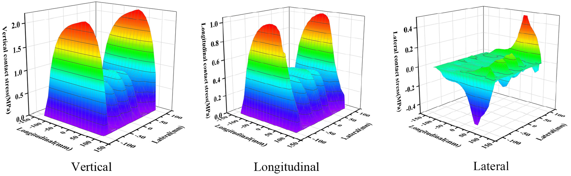
When the inflation pressure is 0.72 MPa and the single tire load is 28 kN, the tire-pavement three-dimensional contact stress is shown as in Figure 19. For comparison, the three-dimensional static contact stress under the same pressure and load conditions is shown in Figure 20.

Figure 19.

Three-dimensional contact stress of free rolling state.

Figure 20.

Three-dimensional contact stress of static state.

It can be drawn from Figures 19 and 20:

The vertical stress distribution of a free rolling tire is dissimilar to that of the static state, although they present a similar saddle-type, and the maximum values are located at the edge of tire, at the same time, the contact stress in the vicinity of the tire center is smaller than the contact stress at the corresponding position in the static state.

The longitudinal stress distribution when the tire is free rolling is quite different from that of the static conditions, and the distribution is antisymmetric in the lateral direction.

When the tire is free rolling, the lateral stress distribution is also quite different from that of the static conditions, and it is distributed asymmetrically on the contact surface.

Acceleration

When the tire angular velocity ω is greater than the free rolling angular velocity ω_l = 43.0588 rad/s, as shown in Figure 14, the tire is in the state of acceleration. As ω continues to increase, the torque and driving force also increase. When ω = 47.9 rad/s, the torque and driving force approach the maximum value. Thus, ω = 46.0588 rad/s is taken as the angular velocity of the acceleration condition.

When the tire inflation pressure is 0.72 MPa and the single tire load is 28 kN, the tire-pavement three-dimensional contact stress is as shown in Figure 21.

Figure 21.

Three-dimensional contact stress of acceleration state.

It can be drawn from Figure 21:

The vertical stress distribution when the tire is in acceleration is dissimilar to the static and free rolling state, although they present a similar saddle-type. However, the maximum vertical stress is located in the back of the tire-pavement surface contact center and not in the center of the tire. The contact stress in the vicinity of the tire center is smaller than that of the corresponding position in the static state.

The longitudinal stress distribution is quite different from that of the static and free rolling state. The longitudinal stress distribution is no longer anti-symmetric in the longitudinal direction under the acceleration conditions, and the value is negative.

Different from the static condition, lateral stress distribution is anti-symmetric in the lateral direction, indicating that the lateral frictional force of the tire under the acceleration condition is smaller than that of the free rolling condition.

Braking

When the tire angular velocity ω is less than the free rolling angular velocity ω_l = 43.0588 rad/s, as shown in Figure 14, the tire is in a state of braking. With the decrease of ω, the torque and acceleration force increase reversely. When ω = 38.1 rad/s, the torque and acceleration force are close to the maximum value. Thus, ω = 40.0588 rad/s is taken as the angular velocity of the acceleration condition.

When the tire inflation pressure is 0.72 MPa and the single tire load is 28 kN, the tire-pavement three-dimensional contact stress is as shown in Figure 22.

Figure 22.

Three-dimensional contact stress of braking state.

It can be drawn from Figure 22:

The vertical stress distribution when the tire is braking is dissimilar to that of the static, free rolling, and acceleration state, different from the acceleration state, its maximum value is located at the front of the tire-pavement contact center. This is because the tire is subjected to the strong friction force of the pavement under braking conditions, and the direction is opposite to the driving direction, resulting in a large deformation in the contact area between the tire and the pavement, the contact surface lags, and the center of gravity of the load moves forward.

The longitudinal stress distribution is completely different from the static and free rolling state, it is similar to the acceleration state, but the longitudinal stress value is positive.

Under the braking condition, the lateral stress presents an anti-symmetric distribution in the lateral direction, and the maximum lateral stress appears at the tire edge. The lateral stress at other positions in the contact area is much smaller than that of the tire edge.

Cornering

Turning of the vehicle is simulated by the cornering of the tire. When the tire is cornering, the friction between the tire and the pavement will limit the tire’s lateral movement, and when the wheel deviates from the straight direction, the tire tread node in the contact area will be deformed laterally.

When the tire inflation pressure is 0.72 MPa and the single tire load is 28 kN, the tire-pavement three-dimensional contact stress at different side slip angles is as shown in Figure 23.

Figure 23.

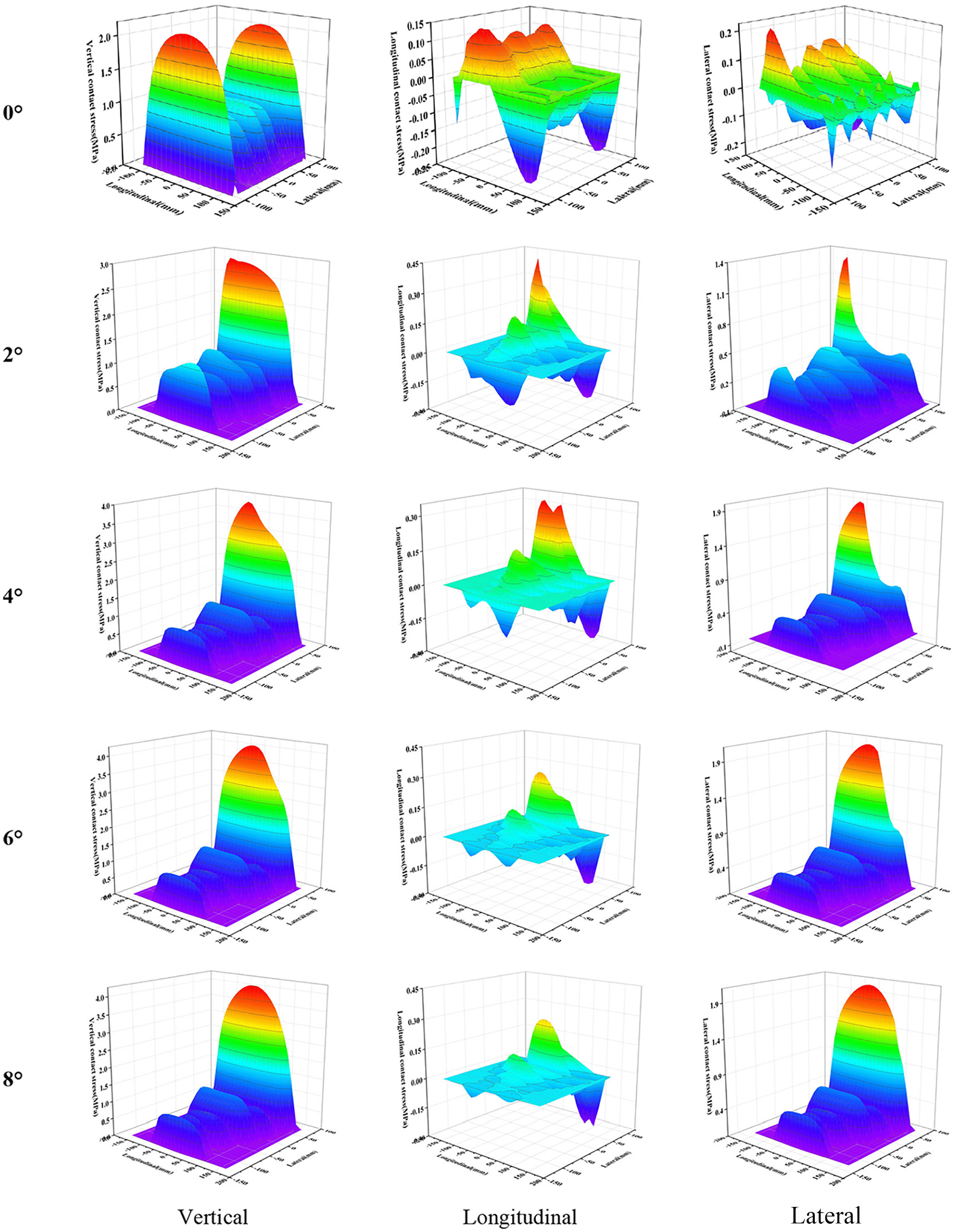
Three-dimensional contact stress of cornering state.

It can be drawn from Figure 23:

When the tire is cornering, the tire shows obvious deformation. The three-dimensional stress moves to the outer side of the tire’s turning direction, and the stress distribution is no longer symmetrical in the center. The maximum value is located at the outer edge of the tire, indicating that the outer side of the tire is subjected to greater compression than the inner side when the tire is cornering.

With an increase of side slip angle, the contact area between the tire and pavement decreases gradually, and the stress concentration is more obvious, which is concentrated in the outer side of the cornering direction.

The vertical stress and lateral stress gradually increase when the side slip angle changes from 0° to 6° and remain basically constant when the side slip angle changes from 6° to 8°, while the longitudinal stress increases when the side slip angle changes from 0° to 2° and gradually decreases when the side slip angle changes from 2° to 8°. The vertical stress and lateral stress in the cornering state are greater than that of the free rolling state.

Figure 24 shows the maximum three-dimensional contact stress under different conditions.

Figure 24.

Maximum three-dimensional contact stress under different conditions.

It can be drawn from Figure 24:

The vertical stress in a state of cornering is the largest, about three times that of a static state and about two times that of free rolling, acceleration, and braking.

The longitudinal stress in a state of braking state is the largest, which is about 3.3 times that of the static state.

The lateral stress in a state of cornering is the largest, about 2.9 times that of a static state, about 9.0 times that of free rolling, 20 times that of acceleration, and 4.2 times that of braking.

Conclusions

In this paper, an 11R22.5 truck radial tire was selected as the research object, the tire three-dimensional model and the tire-pavement contact model were established, the three-dimensional contact stresses distribution under the conditions of static, free rolling, acceleration, braking, and cornering were simulated and analyzed, and the main contributions of the presented work can be summarized as:

The three-dimensional stresses between tire and pavement are significantly affected by inflation pressure, axle load, friction coefficient, and tire driving modes.

Under various conditions, the tire-pavement contact area is similar to a rectangular, and the three-dimensional stresses are non-uniformly distributed rather than in the traditional simplified circular uniform load.

Under a static condition, the ratio of peak vertical, longitudinal, and lateral contact stresses was approximately 1:0.20:0.47.

When the tire is at the state of free rolling, acceleration, braking, and cornering, the three-dimensional contact stresses distribution is different from that of static condition significantly, also, the vertical stress and lateral stress in the state of cornering is the largest, and the longitudinal stress in the state of braking is largest.

In future work, pavement design and damage analysis under three-dimensional contact stress distribution between tire and pavement will be performed based on the findings in this paper.

Footnotes

Handling Editor: Chenhui Liang

Declaration of conflicting interests

The author(s) declared no potential conflicts of interest with respect to the research, authorship, and/or publication of this article.

Funding

The author(s) disclosed receipt of the following financial support for the research, authorship, and/or publication of this article: The authors would like to acknowledge the financial support of the National Natural Science Foundation of China (Grant No. 51978083).

ORCID iD

Jun Xie

References

Prozzi

Luo

. Quantification of the joint effect of wheel load and tire inflation pressure on pavement response. Transp Res Rec 2005; 1919: 134–141.

Machemehl

Wang

Prozzi

. Analytical study of effects of truck tire pressure on pavements with measured tire-pavement contact stress data. Transp Res Rec 2005; 1919: 111–120.

Park

Fernando

Leidy

. Evaluation of predicted pavement response with measured tire contact stresses. Transp Res Rec J Transp Res Board 2005; 1919: 160–170.

Matsuno

Nishizawa

. Mechanism of longitudinal surface cracking in asphalt pavement. In: Proceedings of the 7th International conference on asphalt pavements, Vol. 2, University of Nottingham, UK, August 1992, pp.277–291.

Collop

Cebon

. A theoretical analysis of fatigue cracking in flexible pavements. Proc IMechE, Part J 1995; 209: 345–361.

Myers

Roque

Ruth

. Mechanisms of surface-initiated longitudinal wheel path cracks in high-type bituminous pavements. J Assoc Asphalt Paving Technol 1998; 67: 401–419.

Drakos

Roque

Birgisson

. Effects of measured tire contact stresses on near-surface rutting. Transp Res Rec J Transp Res Board 2001; 1764: 59–69.

De Beer

Fisher

Jooste

. Determination of pneumatic tyre/pavement interface contact stresses under moving loads and some effects on pavements with thin asphalt surfacing layers. In: The 8th international conference on asphalt pavement, Seattle, WA, 10–14 August 1997, pp.179–227.

De Beer

Fisher

. Stress-in-motion (SIM) system for capturing tri-axial tyre–road interaction in the contact patch. Measurement 2013; 46: 2155–2173.

10.

Tielking

Roberts

. Tire contact pressure and its effect on pavement strain. J Transp Eng 1987; 113: 56–71.

11.

Zamzamzadeh

Negarestani

. A 3-D tire/road interaction simulation by a developed finite element model. Akron, OH: Tire Society Conference, 2006.

12.

Zhang

. Nonlinear finite element modeling and incremental analysis of a composite truck tire structure. PhD Dissertation, Concordia University, Canada, 2001.

13.

Meng

. Truck tire/pavement interaction analysis by the finite element method. PhD Dissertation, Michigan State University, USA, 2002.

14.

Wang

Roque

. Three-dimensional finite element modeling of static tire–pavement interaction. Transp Res Rec J Transp Res Board 2010; 2155: 158–169.

15.

Al-Qadi

Wang

. Prediction of tire-pavement contact stresses and analysis of asphalt pavement responses – a decoupled approach. Asphalt Paving Technol 2011; 80: 289.

16.

Wang

Al-Qadi

. Simulation of tire–pavement interaction for predicting contact stresses at static and rolling conditions. Int J Pavement Eng 2012; 13: 310–321.

17.

Zhou

Wang

Ding

, et al. Effect of friction model and tire maneuvering on tire-pavement contact stress. Adv Mater Sci Eng 2015; 2015: 1–11.

18.

Tang

Daniel

Smith

. Numerical evaluation of the temperature field of steady-state rolling tires. Appl Math Model 2014; 38: 1622–1637.

19.

Xue

X-X

Yao

Z-H

, et al. Nonlinear axisymmetric finite element analysis of radial tire. China Rubber Ind 2003; 50: 292–296. (in Chinese)

20.

Sheng

Yimin

Qixian

. Overview of selection and parameter determination for hyperelastic constitutive model of rubber material. Rubber Technol 2018; 16: 5–10– (in Chinese).

21.

Pan

. An investigation on calculation and modeling method for dynamic properties of a rubber isolator. PhD Dissertation, Zhejiang University of Technology, China, 2009. (in Chinese)

22.

Aidy

Hosseini

. A review of constitutive models for rubber-like materials. Am J Eng Appl Sci 2010; 3: 232–239.

23.

Liu

. Finite element analysis on steady state mechanics of all steel radial tire. PhD Dissertation, Jilin University, China, 2006. (in Chinese)

24.

Cui

. Theoretical and experimental research on controllable design for ground performance of radial tire. PhD Dissertation, Harbin Institute of Technology, China, 2016. (in Chinese)

25.

Zhang

. Tire static characteristic finite element analysis and its influence on the vehicle steering stability. ME Dissertation, Zhengzhou University, China, 2011. (in Chinese)

26.

GB/T 2977-2016. China petroleum and chemical industry federation, size designation, dimensions, inflation pressure and load capacity for truck tires. Beijing: China Standards Press, 2016.

27.

Wang

Deng

Shugao

. Finite element analysis of tire-rim contact. Special Rubber Products 2003; 2: 18–21. (in Chinese)

28.

Liu

. Numerical simulation of interaction between tire and asphalt pavement. ME Dissertation, Harbin Institute of Technology, China, 2013. (in Chinese)

29.

Jin

. Study of rolling resistance and temperature profile for radial tire on steady state condition. ME Dissertation, South China University of Technology, China, 2010. (in Chinese)

30.

Feng

Xin

. Finite element analysis on ground contact performance of truck and bus radial tire. Tire Ind 2013; 33: 525–532.

31.

Ford

Yap

. Truck tire/pavement interface. In: The promise of new technology in the automotive industry: XXIII FISITA congress, Torino, Italy, 1990, pp.333–340.

Predictions of three-dimensional contact stresses of a radial truck tire under different driving modes

Abstract

Keywords

Introduction

Finite element modeling of a radial tire

Tire types and parameters

Tire material partition composition

Tire model

Tire rubber material model and parameters

Tire cord ply model

Establishment of tire model

Two-dimensional tire model and meshing

Modeling and assembly of rim

Generation of 3D model of wheel assembly

Tire-pavement contact model

Results and discussions

Static contact analysis

Effect of inflation pressure

Effect of load

Effect of friction coefficient

Dynamic contact analysis

Free Rolling

Acceleration

Braking

Cornering

Conclusions

Footnotes

Declaration of conflicting interests

Funding

ORCID iD

References