
Abstract
Lubrication condition has a strong effect on the service ability of planetary roller screw mechanism (PRSM), so how to effectively identify the lubrication condition of PRSM is highly important in practical industrial applications. A dynamic separable convolution residual convolutional neural network (DSC-RCNN) method is proposed in this paper for the lubrication condition identification of PRSM. In the proposed method, a dynamic separable convolution (DSC) is developed by adopting depthwise separable convolution and dynamic convolution. To verify the learning competence of the proposed method, the PRSM failure test is carried out firstly and vibration data of the PRSM with and without grease are collected in multiple working conditions. Then, three experiments are implemented. The first one is to obtain the optimal number of the depthwise separable convolution in the DSC. The second one compares the effect of the DSC unit and the dynamic convolution unit on the diagnosis capacity of the proposed method. The last one compares SVM, BSA-SVM, AEs, LSSVM, LSTM, VGG-13, and the proposed method. The results reveal the best number of the depthwise separable convolution, the optimal unit of the proposed model and indicate that the DSC-RCNN has enormous recognition and transfer learning abilities.
Keywords
Introduction
Planetary roller screw mechanism (PRSM) is one of the most important and frequently used components in the electromechanical actuator (EMA), which plays a critical role in precision machine tools,1,2 robots, 3 medical equipment, 4 and so on. Effectively detecting the faults of PRSM can provide an assurance for the reliability of machine equipment.
Figure 1 shows the structure of PRSM, containing a screw, a nut, a group of rollers, two annular gears, two carriers, and two circlips. The screw, nut, and rollers with precision threads are key parts that transfer motion and force. With the increase of external load and operating speed, the grease performance on the surface of those transmission parts will degrade gradually. It leads to accelerate wear of those components and the transmission precision loss of PRSM. Hence the lubrication condition has a crucial influence on the performance of the PRSM. In general, detecting the lubrication condition of PRSM is difficult because the transmission components are installed inside the EMA. Therefore, it is essential to establish an intelligent model to achieve the aforementioned purpose.
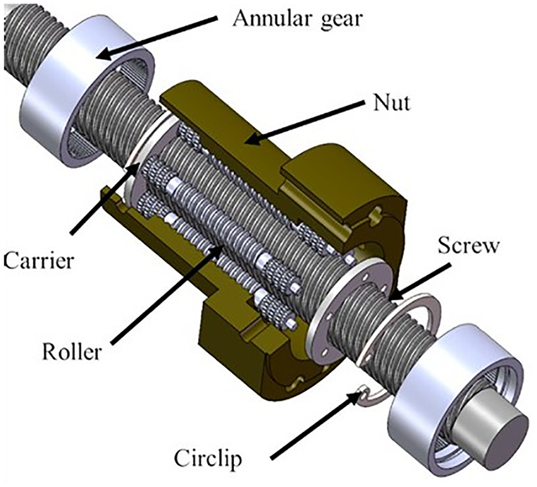
The structure of PRSM.
In the last decades, researches on the PRSM have mainly focused on load distribution,5–7 meshing principle, 8 thermal characteristic analysis,9,10 kinematic analysis, 11 transmission accuracy, 12 and so on. Du et al. 7 established a load distribution model considering the effect of incorporate radial load and machining error. The results showed the load distribution and fatigue life dramatically change with machining errors. Jones and Velinsky 8 used the principle of conjugate surfaces to contact at the screw/roller and nut/roller interfaces in PRSM. It derives the radii of contact on the roller, screw, and nut bodies and makes us know the meshing position of PRSM. Qiao et al. 9 founded a thermal model based on the thermal network method and confirmed the thermal characteristics of the PRSM in various working conditions experimentally. Nevertheless, limited literature has been reported in terms of lubrication condition identification of PRSM. Niu et al. 13 developed a BSA-SVM based on a bird swarm algorithm (BSA) and support vector machine (SVM) 14 to discern the lubrication condition of PRSM. Feature data were extracted artificially from the time domain, frequency domain, and time-frequency domain, respectively, as the input of SVM. BSA was applied to optimize main parameters in the SVM model. Although this method has good recognition ability, it depends strongly on feature data. It will cause that the performance of SVM is directly determined by the quality of the feature data. Therefore, an end-to-end intelligent recognition method which doesn’t rely on manually extracted features needs to be applied in recognizing lubrication condition of PRSM.
At present, plenty of works using machine learning methods to achieve the identification of different states only aim at the same distribution condition. Ezz-Eldin et al. 15 invented a model based on hybrid convolutional neural networks (CNN) and feedforward deep neural networks to automatic speech emotional-speech recognition. Jin et al. 16 created a decoupling attentional residual network for bearing compound fault diagnosis. In those works, the training, validating, and testing data were obtained from the same dataset. The models trained in the same distribution may not get good identification performance in others. Especially for the PRSM, the data in different working conditions have different distributions. It implies that the models trained in one working condition are not suitable for others. In addition, it is difficult for the PRSM to acquire data under various working conditions. Therefore, it is significant to handle the domain shift problem about recognizing lubrication condition of the PRSM. This knowledge learning process in different domains is denoted as transfer learning. Figure 2 displays the differences between machine learning and transfer learning. The nature distinction is that the training and test data in the transfer learning are from different domains in the different distributions. Consequently, how to improve the performance of transfer learning is crucial to an intelligent recognition method.

A comparison between machine learning and transfer learning.
Therefore, to settle the above needs this paper develops a novel method based on dynamic separable convolution RCNN (DSC-RCNN) to identify the different states of grease in the PRSM. The dataset with and without lubrication is collected from the PRSM fault bench test to explore the proposed method’s discerning competence and transfer learning ability in different working conditions. The influence of the parameter k in the dynamic separable convolution on the developed method is discussed. The performance of the developed method is compared with SVM, BSA-SVM, autoencoders (AEs), 17 least square SVM (LSSVM), 18 long short-term memory (LSTM), 19 and VGG-13. 20 The highlights of this paper are summarized below.
An end-to-end intelligent learning method is proposed for the lubrication condition monitoring of PRSM in different working conditions.
A dynamic separable convolution is developed to increase the representation capability without increasing the extra parameters.
A basis unit based on a dynamic separable convolution and a shortcut layer is introduced into the proposed method in order to enrich the extracted characteristics.
The transfer learning of the proposed method is validated for lubrication condition monitoring of PRSM and compared with the existing techniques in a real-world dataset.
After introducing the characteristics of PRSM and the importance of lubrication conditions to work performance of the PRSM in Section 1, Section 2 mainly proposes a dynamic separable convolution (DSC) instead of traditional convolution to improve the prediction performance. Section 3 briefly describes the DSC-RCNN structure based on DSC blocks and pooling layers. The experiment of PRSM in working conditions, including different loads and speeds, is carried out and provides data to verify the learning ability of the corresponding proposed method in Section 4. And the performance of the proposed method is experimentally validated. Finally, the conclusions are presented in Section 5.
Dynamic separable convolution
In this section, a novel dynamic separable convolution based on depthwise separable convolution and attention is introduced to provide better trade-off between network performance and computational burden. Figure 3 describes the inner structure of DSC in detail. The DSC mainly is made up of attention, point convolution, depth convolution, Batch Normalization (BN), and ReLU. The attention includes two standard convolution layers, a dimensionality reduction layer and an activation function layer.

A dynamic separable convolution.
The coefficient vector

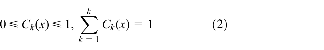
where

where
In the DSC the depth convolution and the point convolution are 2D standard convolution. The number of the convolution kernels in the depth convolution is same as the channel number of the input
In addition, the DSC adopts two standard convolution operations to obtain coefficient vector
Network architecture design
This subsection introduces an end-to-end network structure for PRSM fault signal classification problems. The flow chart is presented in Figure 4. This RCNN method mainly includes eight DSC blocks, four pooling layers, a BN layer, and a fully connected (FC) layer.

The network architecture of DSC-RCNN.
DSC block
Convolution operation can extract and combine feature data hierarchically. With increasing convolution layers, the extracted information is richer and more relevant. However, the training of deep neural networks is not a process of stacking simply. The deeper the network, the more prone it is to gradient explosions and gradient disappearance. Consequently, this paper employs a shortcut layer in the DSC for addressing those aforementioned problems.
As shown in Figure 5, two kinds of basic units for the CNN method are taken into account. The DSC unit comprises a shortcut layer, a DSC, a BN layer, and a ReLU layer.

Two kinds of basic units for the method.
The output of DSC unit is described as follows.

where
In the DSC, a shortcut layer adds the raw low-level features directly across the multilayer network to the high-level features to rich the extracted data features. The output of the shortcut layer is described as follows.

Whereas the dynamic convolution (DC) 21 unit in Figure 5 adopts a shortcut layer combined with a DC that replaces separable convolution with standard convolution.
The output of the DC unit is given as follows.

where
In Figure 5 it is clear that the output channels of the DSC or DC and the shortcut layer are the same to do addition. As far as we all know, the BN layer and the ReLU layer don’t change the output size. Hence, the output channels of those units are equal to that of the DSC or DC. In addition, the kernel size of the shortcut layer is 1 × 1 to obtain the raw low-level features as possible.
The DSC/DC block is made up of two those basic units in Figure 6. The size of input features is the same as that of output features. Only the channel number of input features changes from C to O.

The architecture of the DSC block.
Reshaped data
Due to the two-dimensional convolution operation in this paper, the one-dimensional input must be reshaped to a two-dimensional signal. The processing methods, such as wavelet packet transform, wavelet transform, and Fourier transform, are adopted to artificially extract features and reshape data. Although those methods are applied successfully in video processing and fault diagnosis, the processing inevitably increases the computation time. Hence, in this paper the two-dimensional samples are formed by directly taking a sort segmental data from a raw signal and organizing it in a row fashion.
Pooling layer
A pooling layer22,23 is used widely in neural networks to realize data volume decline and relieve computational pressure. In this paper average the pooling layer is utilized because it doesn’t need parameters and can reduce the risk of overfitting in the training of the neural network.
Batch normalization layer
In neural network, a BN 21 layer can make the distribution of eigenvalues normalized. This could not only speed up the training process but also accelerate the convergence of the network model. The process of BN layer is described as follows.
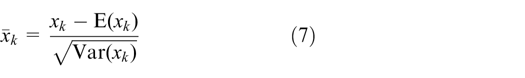

where E(xk) and Var(xk) represent the mean and variance of the eigenvalues of a layer, respectively. γk and βk are a pair of parameters which scale and shift the normalized value yk.
Fully connected layer
Generally, a FC layer 24 is placed in the last layer in neural network to map the data features learned by the front layers into sample space. So a FC layer in this paper is utilized to reduce data dimensions and output classification results.
Cross-entropy loss
Cross-entropy loss 25 is usually used to describe the distance between the real probability distribution and the predicted probability distribution in classification tasks.
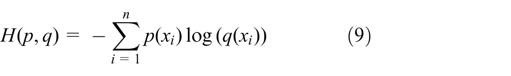
where p(xi) is the real label for the training set and q(xi) is the label value predicted by the network.
Network parameters
The network parameters of the proposed method and the feature map size after each layer are clearly exhibited in Table 1. K and C are kernel sizes and convolution channels.
Network parameters of dynamic separable convolution RCNN.

Experiments
Data collection
To evaluate the performance of the proposed recognition method, the experiment of PRSM in two states is carried out. Figure 7 indicates the lubrication states of PRSM with and without grease.
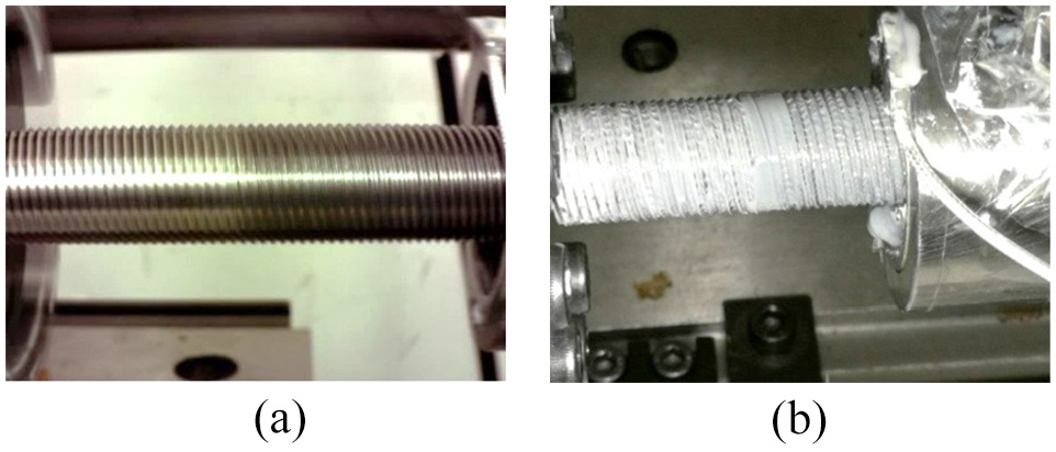
The lubrication states of PRSM: (a) without grease and (b) with grease.
The data is collected from the PRSM failure test bench, as shown in Figure 8. The test bench is composed of a servo motor, a reducer, a PRSM, a vibration acceleration sensor, and a hydraulic system. The servo motor is connected to the input end of the PRSM through the reducer to provide power for the PRSM. The hydraulic system is directly connected with the output end of the PRSM to simulate the loading process of the PRSM. During the experiment, the PRSM drives the hydraulic system to produce reciprocating motion so as to realize active loading. The vibration acceleration sensor is placed on the nut of the PRSM to collect the vibration characteristics of the whole system as it moves. The rated power of the servo motor is 5000 W. The diameter of the screw in the PRSM is 25 mm.

The PRSM failure test bench.
The sampling frequency of the data acquisition card is set to 20,480 Hz. Data acquisition is carried on every 0.1 s. Each vibration signal sample contains 2048 data points. The collected data has three channels, respectively representing the three directions of PRSM. Eight working conditions are listed in Table 2. In the experimental process, the movement of the PRSM is controlled to make its displacement curve appear triangle wave so as to ensure that its speed is uniform in the reciprocating movement. The stroke of the reciprocating motion is set to 70 mm. The raw signal of PRSM without and with grease is collected as shown in Figures 9 and 10.
The working condition of PRSM.


The raw signal of PRSM without grease.
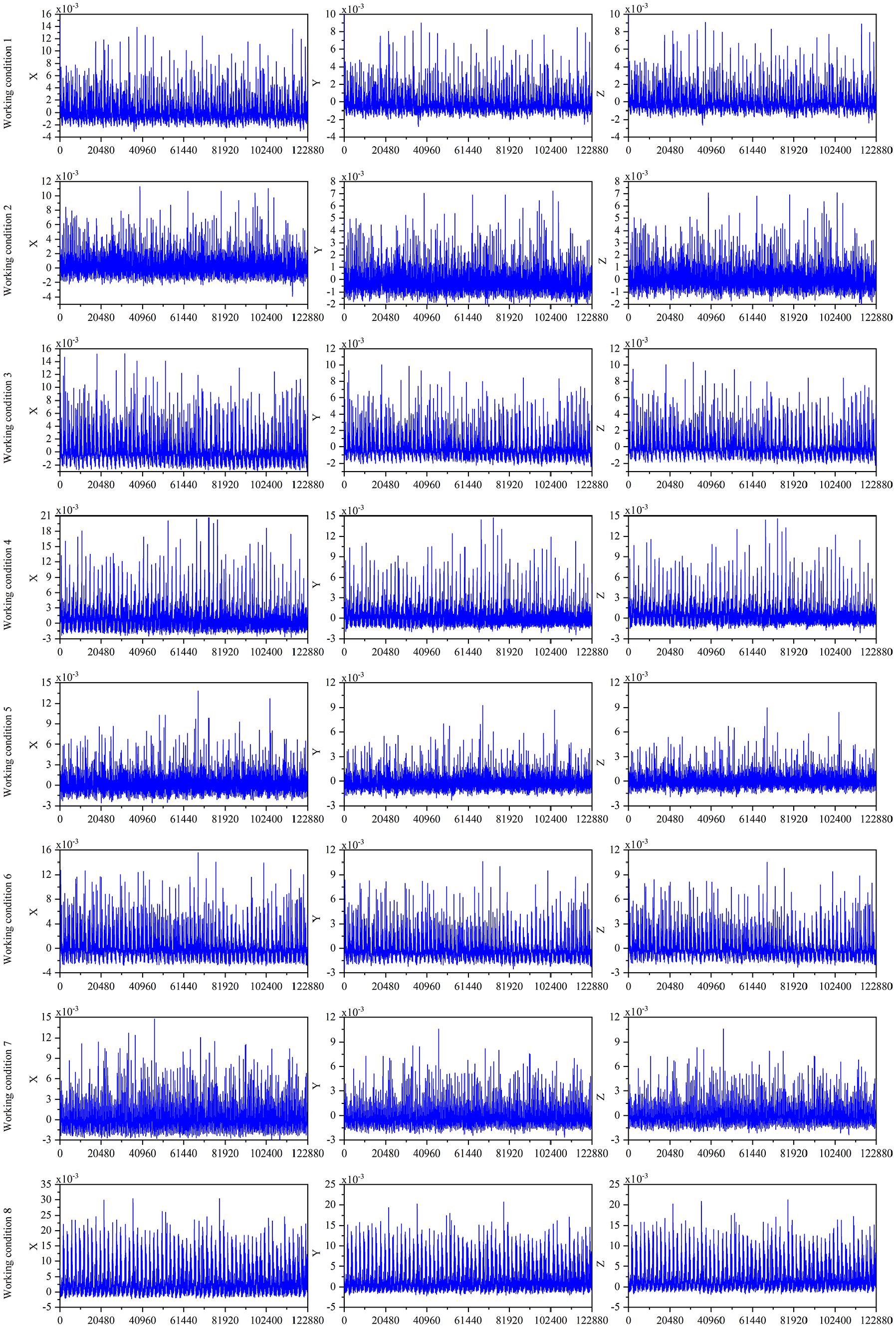
The raw signal of PRSM with grease.
Data preparation
Due to the limited data samples, data augmentation26,27 is used to increase samples in the training process. This method makes use of overlapping samples and shift transformation. As shown in Figure 11, the process of overlapping sample is described vividly. Every two adjacent samples have an overlapping sample. The number of the overlapping samples is shift length. In this paper, the shift length is 128, the sample data length is set to 1024, and the sample number changes from 60 to 480. To avoid occasionality, 80% of the dataset in each working condition is randomly divided into the training samples, 10% of the dataset is validating samples, and the rest is testing samples. As a result, the training, validating, and testing samples are totally 6144, 768, and 768.

The process of overlapping sample.
To test the transfer learning competence of the proposed model, one of the eight working conditions in turn is treated as a testing set. The rest is divided into a training set and validating set according to the ratio of 9:1. So the sample numbers of a training set, validating set and testing set are 6048, 672, and 960.
Discussion and analysis
The effect of the number of the depthwise separable convolution
The effect of the number k of the depthwise separable convolution on the proposed network is discussed because of having a great influence on the complexity of the model. Considering the scale and effectiveness of the network, predicted results of the model are analyzed when k is 2, 4, 6, and 8.
The models in different k are examined by testing set. Figure 12 shows the testing accuracy and the area under receiver operating characteristic (ROC) curves in different k. It is evident in Figure 12 that this method can precisely discern the lubrication condition and the testing accuracies in different k are 100%, 100%, 100%, and 99.74%, respectively. In addition, Figure 12 shows the area under ROC curve (AUC) of the different k is 1. It suggests that the proposed method has good diagnostic authenticity in spite of the different k.

The testing result of DSC-RCNN in different k.
In different working conditions, the testing accuracy of transfer learning in different k is shown in Table 3. The testing accuracies of the different working conditions are higher than 97%. It indicates that the proposed method also has good transfer learning ability. Particularly, when k is 8, the testing accuracies in different working conditions are all higher than 98% and the fluctuation of testing accuracies is smaller. Figure 13 describes the testing AUC of transfer learning in different k. The values of AUC in different k are higher than 0.994. It implies that the models of the different k all have very reliable identification ability.
The transfer learning accuracy of DSC-RCNN in different k.


The transfer learning AUC of DSC-RCNN.
Although the average accuracy of k = 8 in transfer learning is 0.04% higher than that of k = 4, the testing accuracy of k = 8 is 0.24% lower than that of k = 4. And the network structure parameters of k = 8 is more than that of k = 4. As a result, the number k of the depthwise separable convolution is set as 4 considering the network structure parameters and predicted results of the method.
The predicted effect of the DSC block and the DC block on the method
The DC-RCNN model is based on the DC block and the RCNN model. After training process, the testing results of the DC-RCNN model in different k are compared with the DSC-RCNN model in Figure 14(a) that the testing accuracies of the DC-RCNN are decreasing with k. What’s more, the testing accuracies of the DC-RCNN in different k are lower than that of the DSC-RCNN.

The testing results of the DC-RCNN and the DSC-RCNN in different k: (a) the testing accuracy and (b) the testing AUC.
The AUC of DC-RCNN and DSC-RCNN in different k is presented in Figure 14(b). The values of AUC in the DC-RCNN are all higher than 0.98 in different k but lower than that of DSC-RCNN. It proves that the DC-RCNN model is not good as the DSC-RCNN model in the identification learning process.
Next, to further compare the transfer learning ability in the DC-RCNN and the DSC-RCNN, the predicted accuracy of DC-RCNN in transfer learning is illustrated in Table 4. When k is 2 the testing accuracy of the DC-RCNN is the highest in those working conditions and all higher than 95%. At the same time, in Table 5, the transfer learning AUC of DC-RCNN in k = 2 is higher than that of other k in all working conditions. However, by contrasting Table 3 with Table 4, the predicted accuracy of the DC-RCNN in k = 2 is less than the DSC-RCNN. And the AUC of the DC-RCNN is also inferior to that of the DSC-RCNN by comparing Figure 13 with Table 5. Therefore, the transfer learning ability of DSC-RCNN is superior to that of the DC-RCNN.
The transfer learning accuracy of DC-RCNN in different k.

The transfer learning AUC of DC-RCNN in different k.

In a word, the DSC-RCNN has better recognition performance and transfer learning performance compared with the DC-RCNN.
Diagnosis results of different methods
In order to further evaluate the performance of the proposed method, different models are implemented for comparisons.
SVM
In the SVM, 14 the kernel function is the Gaussian Radial Function kernel. Kernel parameter g and penalty parameter c are set as 0.5 and 1.
BSA-SVM
In the BSA-SVM, 13 the same kernel function as the SVM model is chosen. The range of kernel parameter g and penalty parameter c is set as [0, 100], population number and iteration number are 30 and 50 in BSA-SVM.
AEs
The AEs 17 model is employed to extract features and the output of the encoder block is input into a linear classifier. The output channels of the classifier layer are the numbers of the discerning classes.
LSSVM
In the LSSVM, 18 the RBF kernel function is chosen. The regularization parameter and kernel parameter are 10 and 0.3.
LSTM
In the LSTM, 19 the input feature is 32 and the hidden feature is 100. The LSTM can extract hidden feature about time from a time domain signal.
VGG-13
The VGG-1320 is chosen mainly due to taking into account the influence of the input size and the model depth. Because of the difference of the input size and the identification variety, the linear classifier of the VGG-13 is replaced by those three FC layers that the weight of those is 512 × 256, 256 × 256, and 256 × 2.
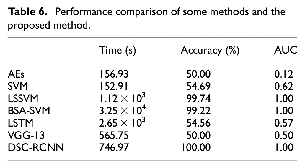
The predicted results of different methods are shown in Table 6. Table 6 indicates testing accuracy of the proposed method is the highest. Although the running time of the SVM is the least, the identification result is terrible. The predicted results of the AEs, the VGG-13, and the LSTM are also bad. The BSA algorithm can improve the recognition ability of SVM. Nonetheless, the optimization will spend so much time on parameters selection of SVM. And the BSA-SVM optimization process implies that the classification ability of SVM has tremendous relevance to parameters of the kernel function. This trouble will exist all the time in the SVM model. The LSSVM can enhance the predicted accuracy. Whereas it costs more time than the proposed method and the accuracy of the LSSVM is also lower than that of DSC-RCNN in k = 4. As a result, the recognition competence of the proposed method is the best in those available algorithms.
Performance comparison of some methods and the proposed method.
Furthermore, the comparison of the transfer learning in above models is shown in Tables 7 and 8. Table 7 shows us that the DSC-RCNN in the different working conditions also has better transfer learning competence. The predicted average accuracy of the DSC-RCNN in the different working conditions is 99.62% and the highest compared with other methods. Although the LSSVM also has good identification competence, the predicted accuracies are lower than that of the DSC-RCNN. In Table 8 the values of the AUC in DSC-RCNN and LSSVM are 1. It implies that the DSC-RCNN and LSSVM have good generalization abilities.
The transfer learning accuracy of the DSC-RCNN and those compared models in different working conditions.

The transfer learning ROC of the DSC-RCNN and those compared models in different working conditions.

As a summary, compared with SVM, BSA-SVM, LSTM, AEs, LSSVM, and VGG-13, the developed DSC-RCNN achieves comprehensive performance and is able to identify the lubrication condition of the PRSM.
The comparison of the different methods in gear fault data
To further verify the property of the DSC-RCNN in other dataset, the fault data set of 3 MW wind turbine pinion gear by Eric Bechhoefer 28 is utilized. This data set includes 11 fault data files and 13 good condition data files. The fault data is obtained from a fault 3 MW wind turbine pinion gear. Those good condition data are given from pinion gears of different wind turbines of the same model. Those data have two channels and is a record of the radial vibration accelerometer and the tachometer. In this training process, only the vibration data is used. The sample rate of the vibration data is 97656 Hz. The record length is 6 s. The testing results comparison of the above methods is displays in Figure 15.

The testing results of the DSC-RCNN and those compared models in the gear fault data set.
The predicted accuracy of the LSSVM, the LSTM, the VGG-13 and the proposed method all is 100%. And the values of AUC in those methods are 1. It indicates that the proposed method still has good identification competence.
Visualization of the network learning process
A convolutional neural network is similar to a black box, so the internal process cannot be reasonably explained. To clearly understand the internal learning process of the network, the T-SNE method 29 is used to reduce the dimension of the middle output result and displays the middle result in the lower dimension. The visualization is depicted in Figure 16.

The visualization of the predicted results of DSC-RCNN: (a) original data, (b) 40 iterations, (c) 70 iterations, and(d) 100 iterations.
Figure 16 shows the visualization of the output result in validating process of the DSC-RCNN. The data with grease and without grease is chaotic and not identified before the training of the network. But after 40, 70, 100 iterations, it is obvious that the validating set can be easily divided. Consequently, the visualization directly confirmed the recognition capability of the proposed network.
Conclusions
In this paper, an effective lubrication condition identification method, called DSC-RCNN, for the PRSM is proposed. In order to verify the diagnosis performance of the method, vibration acceleration data of PRSM with and without grease is collected from the PRSM failure test bench and preprocessed by data augmentation. Three analysis of the DSC-RCNN are conduct. The conclusions are present as follows.
The effect of the number of the depthwise separable convolution k in the DSC on the predicted accuracy is discussed, when k is 2, 4, 6, and 8. The results shows the optimal number of the depthwise separable convolution is 4 in the DSC-RCNN.
The learning ability of the RCNN based on DC blocks is analyzed. It shows that the maximum difference of transfer learning accuracy between DSC-RCNN and DC-RCNN is 13.82%.
The effectiveness of the proposed PRSM lubrication condition identification method is confirmed by comparison with AEs, SVM, LSSVM, BSA-SVM, LSTM, and VGG-13. The recognition accuracies of DSC-RCNN are 50.00%, 45.31%, 0.26%, 0,78%, 45.44%, 50.00% higher than that of the above models, respectively. And the transfer learning accuracies of DSC-RCNN are also 49.62%, 45.23%, 0.79%, 8.02%, 44.80%, 49.62% higher than those.
As a result, the DSC-RCNN for lubrication condition identification of PRSM has robust recognition ability and fine facticity.
Footnotes
Handling Editor: Chenhui Liang
Declaration of conflicting interests
The author(s) declared no potential conflicts of interest with respect to the research, authorship, and/or publication of this article.
Funding
The author(s) disclosed receipt of the following financial support for the research, authorship, and/or publication of this article: The research was supported by National Natural Science Foundation of China (Grant No. 51875458), Key Research and Development Program of Shaanxi (Program No.2021ZDLGY10-08), and Natural Science Basic Research Plan in Shaanxi Province of China (Grant No.2020JQ-178).