Control of a DC motor using feedback linearization and gray wolf optimization algorithm

Abstract

The aim of this study is to investigate nonlinear DC motor behavior and to control velocity as output variable. The linear model is designed, but as it is experimentally verified that it does not describe the system well enough it is replaced by the nonlinear one. System’s model has been obtained taking into account Coulomb and viscous friction in the firmly nonlinear environment. In the frame of the paper the dynamical analysis of the nonlinear feedback linearizing control is carried out. Furthermore, a metaheuristic optimization algorithm is set up for finding the coefficient of the proportional-integral feedback linearizing controller. For this purpose Gray wolf optimization technique is used. Moreover, after the introduction of the control law, analysis of the pole placement and stability of the system is establish. Optimized nonlinear control signal has been applied to the real object with simulated white noise and step signal as disturbances. Finally, for several desired output signals, responses with and without disruption are compared to illustrate the approach proposed in the paper. Experimental results obtained on the given system are provided and they verify nonlinear control robustness.

Introduction

Direct current (DC) motors are mostly used in industries where velocity is required to keep accurate adaptation, or where low-velocity torque is needed, for example electric vehicles, steel rolling mills, electric cranes, and robotic manipulators due to precise, wide, simple, and continuous control characteristics. ¹ Also, it is extremely important to describe the response feature and fatigue life of certain structures. ² As manufacturing sector represents the first momentum of Energy-Based Maintenance evolution, and technology transfer activities are necessary, ³ it is of great importance to research well and know all the possibilities, elements, and machines that drive production. There are several possibilities within brushed motors. One with the permanent magnet, shunt, series, and combination of the last two-compound. They are all suitable for usage in different applications in industry. This paper investigates series wound DC motor which can supply varying voltage.

Many different techniques can be applied to control the velocity of the output series DC motor shaft. Frequently used are, surely, conventional methods such as traditional feedback control: proportional-integral-derivative (PID) like controllers. They have low prices (compared to more complicated control systems), they are simple and different variants of this control systems (proportional-integral PI or proportional-derivative PD) manage to keep the output of the system well matched with the set value within the error limits. On the other hand, they suffer due to lack of robustness. ⁴

Other than conventional, there are many nonlinear controllers. Some of them use adaptive control technique, because the estimated velocity is heavily contaminated by noises from the switching signals. This direct method nullifies the merit of the sliding mode observer. ⁵ In order to overcome the boundaries of model reference adaptive control several are built from Artificial Neural Network (ANN), like it was proposed in the papers.^6,7 ANNs enable estimating and controlling velocity for a separately excited DC machine and it is one of the most important modern techniques. The rotor speed of the machine can be made to follow an arbitrarily selected trajectory, especially when the motor and load parameters are unknown. In Alhanjouri ⁸ these two neural networks are trained by Levenberg-Marquardt back-propagation algorithm. Simulation results indicates to the advantages, effectiveness, good performance of the artificial neural network controller, which is illustrated through the comparison obtain by the system. In nonlinear system, self-tuning ANNs technique is related to linearization of model at operating time interval. This may produce error because of linearization of nonlinear model and cannot control the speed accurately. ¹

In general, the control of system is difficult due to high nonlinearity properties. To overcome this difficulty, another technique, which include Fuzzy Logic Controller (FLC) can be developed. ⁹ FLC is just one of the intelligent controllers and represents a widespread control technique as it has satisfactory performance for nonlinear and complex systems. Basic character and the aim of this control strategy is to take advantages of knowledge and the control experience of the operator for intuitive synthesis of the control system. Analysis and comparison with classical PID control, sliding control, adaptive control, etc., that is, by conventional control techniques, have led to the results which were also used for the analysis of stability and quality of dynamic behavior. ¹⁰ The fuzzy design can be considered as an optimization problem, where the structure, antecedent, and consequent parameters are required to be identified.

Global optimization problems are difficult to be solved efficiently because of their high nonlinearity and multiple local optima. Nonetheless, with nonlinear equations it is senseless examining system’s stability, but one can check the stability of the separate equilibriums. System which has two equilibrium points can initially be in equilibrium number one, which is unstable. When the disturbance is applied, it can happen that the second equilibrium attracts trajectory and the state can converge in the second equilibrium. ¹¹ Therefore it is necessary to check whether the global minimum time of motion is actually realized by the obtained solution. ¹² Finding the optimal solutions represent the basic and challenging task, that is widely studied for decades. Nature has been a major source of inspiration for researchers in the field of optimization. ¹³

The implementation of metaheuristic algorithms can be solved with nonconvex, nonlinear, and multimodal problems subjected to linear or nonlinear constraints by continuous or discrete decision variables, in the form of global optimization algorithms. For example, differential evolution and genetic algorithms have been used to perform an optimal design of a phase controller to track the trajectory of moving robots.^14–16 Some of these algorithma include the genetic algorithm (GA), ¹⁷ particle swarm optimization (PSO), ¹⁸ whale optimization algorithm (WOA), ¹⁹ gray wolf optimization (GWO), ²⁰ etc. Based on ²⁰ GWO technique illustrates its supremacy with an improved version of GWO technique named as IGWO. This controller was proposed and demonstrated for step load disturbances, stochastic load disturbances, and varied conditions. In combination with other nonlinear control systems, these Park et al. ²¹ as well as the other techniques such as ant colony (AC) ²² and a novel method called the cuckoo search (CS) ²³ can be applied.

Although modeling a nonlinearity is often a very complicated challenge, one of the first steps in the synthesis of a control system is to create a mathematical model. This will save time and bring the cost-effectiveness. ²⁴ On the other hand, an exact mathematical models can not be easily obtained. One way to battle this kind of problem is given in the paper which used real coded genetic algorithm with a goal to estimate the unknown system parameters. In order to integrate the resulted system model and the feedback linearizing controller (FBL), the nonlinear robotic system can be transferred to a linear model with a nonlinear bounded time-varying uncertainty. ²⁵

Feedback linearization is the nonlinear control technique which has attracted increasing attention in past decades. ²⁶ By a synergy of a nonlinear transformation and linearization with feedback loop, the nonlinear control design allows the creation of linear control law. ²⁷ The central idea of the approach is to algebraically transform a nonlinear system dynamics into a (fully or partly) linear one, so that linear control techniques can be applied. This differs entirely from conventional linearization in that feedback linearization is achieved by exact state transformations and feedback, rather than by linear approximations of the dynamics. ²⁸ This technique has been successfully implemented in many applications of control, such as industrial robots, high performance aircraft, helicopters, and biomedical dispositifs; more tasks which used this methodology are being now well advanced in industry. ²⁹ In Cambera and Feliu-Batlle ³⁰ the problem of tracking the trajectory of the flexible end effector was solved using FBL method, where the force of gravity and the force of joint friction are taken into account. As relatively simple and easy understandable technique FBL is suitable to be used in nonlinear systems: Aerial Package Delivery Robot, ³¹ manipulators, ³² and even for a high-DOF robots. ³³

An optimal control strategy for a bearingless permanent magnet synchronous machine drive is proposed in Sun et al. ³⁴ The state feedback control (SFC) based on the GWO algorithm is applied. The discretized state model with the augmented integrals of the displacement error and angular speed error is obtained. Then, the weighting matrices are obtained by employing the GWO algorithm. The results show the superiority of the proposed method reflecting in faster response and no overshoot compared with the PI controllers. On the other hand, paper ³⁵ presents an optimal control strategy for a permanent-magnet synchronous hub motor (PMSHM) drive using the state feedback control method plus the gray wolf optimization (GWO) algorithm. To acquire satisfactory dynamics of speed response, the discretized state space model of the PMSHM is augmented with the integral of rotor speed error and integral of current error. Then, the GWO algorithm is employed to acquire the weighting matrices Q and R in liner quadratic regulator optimization process. Finally, comparisons among the GWO-based state feedback controller, the conventional state feedback controller, and the genetic algorithm enhanced PI controllers are conducted in both simulations and experiments. The comparison results show the superiority of the proposed state feedback controller with the penalty term in fast response. Finally, ³⁶ proposes an improved deadbeat predictive controller for PMSM drive systems. It can eliminate the influence of parameter mismatch of inductance, resistance, and flux linkage. A composite sliding mode disturbance observer (SMDO) based on stator current and lumped disturbance is proposed, which can simultaneously estimate the future current value and lumped disturbance caused by the parameter mismatch of inductance, resistance, and flux linkage. Both simulation and experimental performances of the proposed method have been validated and compared with the conventional control methods under different conditions. The comparison results show the superiority of the proposed predictive current control method based on the composite SMDO.

In this paper, the FBL method was used to control the velocity of the DC motor. The feedback linearization is a powerful nonlinear method based on the principle of canceling the nonlinearities of the system model. In most papers dealing with the similar topics of FBL technique application for DC motor control (see Mehta and Chiasson, ²⁷ Moradi et al., ³⁷ Shirvani Boroujeni et al. ³⁸ ) the nonlinear model is made on the basis of flux and motor current nonlinearities. For the purposes of this research, feedback linearization was performed using a mathematical model that takes into account the nonlinearity resulting from friction. Therefore, a nonlinear mathematical model of a DC motor with previously determined friction, in the form of a Tustin model, was adopted. Moreover, a new model was applied in which the discontinuous nonlinearity was approximated by a differentiable nonlinearity of the hyperbolic tangent, which ensured the conditions for the application of FBL. After the feedback linearization method has been successfully utilized to change the nonlinear states of the system to their linear forms, classical PI controller has been implemented for DC motor velocity control. Determining controller gains has been considered as an optimization problem and solved using GWO optimization algorithm, as one of recent metaheuristics swarm intelligence methods. GWO has been widely tailored for a wide variety of optimization problems due to its impressive characteristics over other swarm intelligence methods: it has very few parameters, and no derivation information is required in the initial search. Also it is simple, easy to use, flexible, scalable, and has a special capability to strike the right balance between the exploration and exploitation during the search which leads to favorable convergence. ³⁹ The last contribution of the paper is the demonstration of robustness and good control performances of nonlinear system control against external disturbance and in the presence of noise, through experimental results.

Description of the system

In this Section from the electrical, mechanical, and combined equations we obtain and investigate linear model of the DC motor . Mathematical model and discussion of the model benefit is conducted. Here the experimental verification of the obtained mathematical representation is provided.

The first prominent pace in control design is obtaining the most precise model possible, because it reduces time for task performing. Furthermore, it brings the labor saving, cost-effectiveness, and makes work easier and faster. That is why establishing the valid model is a crucial stage in the practical control problems.

The main aim of modeling DC motor is to find the applied voltage, torque, current, or speed related differential equations. ⁴⁰ Object is taken to be the DC motor, SRV02 Rotary Servo Base Unit, which has been considered as a single-input-single-output (SISO) system. This object is equipped with the optical encoder and tachometer, for motor position and speed measuring, respectively. ⁴¹

A schematic diagram of this series wounded DC motor is given in the Figure 1, where $V_m$ , $e_b$ , $k_m$ , and ${\omega }_m$ are motor voltage, back electromotive voltage, back electromotive voltage constant, and speed of the motor shaft, respectively.

Figure 1.

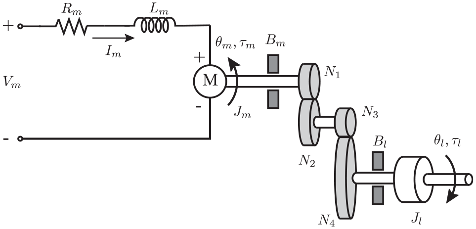
Schematic diagram of the DC motor. ⁴¹

As given in the specifications, it is assumed that in the electronic circuit inductance $L_m$ is much smaller than the resistance $R_m$ , and therefore it does not figure in the equations. ⁴¹

Linear model of DC motor

The well known linear equation of a DC motor is obtained by combining electrical and mechanical equations and assuming that motor torque is proportional to the voltage.

Choosing the velocity of the load shaft ${\omega }_l=\omega$ as output variable $y=\omega$ and $u=V_m$ as input variable, linear model of the system is obtained as follows:

$$J_{\mathrm{eq}}\frac{d}{\mathrm{dt}}y(t)+B_{\mathrm{eq},v}y(t)=A_{m}u(t).$$

(1)

where: $J_{\mathrm{eq}}$ is total moment of inertia calculated as: $J_{\mathrm{eq}}={\eta }_g{K}_g^2{J}_m+J_l$ ( ${\eta }_g$ and $K_g$ are, respectively, the gearbox efficiency and the total gear ratio, $J_m$ is moment of inertia of the motor shaft and $J_l$ of the load), the equivalent damping term is given by $B_{\mathrm{eq},v}=\frac{{\eta }_g{K}_g^2{\eta }_m{k}_t{k}_m+({\eta }_g{K}_g^2{B}_m+B_l)R_m}{R_m}$ ( ${\eta }_m$ is the motor efficiency, $k_t$ is the current-torque constant, $B_m$ and $B_l$ are viscous frictions acting on the motor shaft and on the load shaft), and finally the actuator gain which equals $A_m=\frac{{\eta }_g{K}_g{\eta }_m{k}_t}{R_m}$ , Table 1.

Table 1.

The numerical values of the DC object.

Parameters	Values and units
$J_{\mathrm{eq}}$	0.0021  $\mathrm{kg}{m}^2$
$R_m$	2.6  $\Omega$
$k_t$	0.0077  $\frac{\mathrm{Nm}}{A}$
${\eta }_m$	0.69
${\eta }_g$	0.9
$K_g$	70

A DC series motor can serve as a vehicle for the evaluation of the performance of the various controllers. ⁴²

Experimental confirmation of the acquired mathematical representation

Responses of the system are given in the following: Figures 2 and 3. Comparisons were made with the responses obtained by simulations of the linear model, for step and sinusoidal inputs. The responses of the real object and the linear model to the step and sinusoidal excitations do not match well. The model does not follow the actual behavior of the system. Decreasing the amplitude changes only the sign of the deviation. This is because the system is not linear and homogeneity principle could not be applied.

Figure 2.

Comparison between real and model output for two step inputs: lower with amplitude 0.3 and higher with amplitude 5.

Figure 3.

Comparison between real and model data for sinusoidal input, amplitude 1 and frequency 0.5 rad/s.

The nonlinearity in the form of the dead zone can also be seen in the sine wave. This nonlinearity represents the effect of the friction. It is special expressed in low-frequency sinusoidal functions (and with change of the rotation direction), because then the effect of the friction is most noticeable. It is easy to see that the linear model fails to replicate the response of the system.

Friction phenomenon is the cause of many failures in mechanical parts of mobile systems, and compensation can be encouraged by various constructive solutions, but they do not eliminate nonlinearities at low speeds. In order to obtain the most accurate model of a DC motor and to enable a good synthesis of the control system later, it is necessary to consider and take into account the nonlinearity of friction.

Feedback theory derivation and relative degree of the system

In the following two sections, we will look at the theoretical derivations related to the subject: FBL and GWO algorithms. We will going to need those derivations in order to better understand behavior of the control synthesis, which will be capable of rejection the disturbances in machines.

System described by linear differential equations in the state space is always possible to solve analytically. On the other hand, when an engineer comes across nonlinear equations it is almost regularly impossible to reach an analytical solution. Then, the solution can only be sought numerically.

However, very often, especially when designing, it is convenient to have an analytical solution or at least some analytical guarantees about what the solution looks like. This is important primarily when choosing parameters, because then one can judge in advance, without some complex computational operations, how changing a parameter affects the behavior of the whole system.

Linearization is usually done around the desired equilibrium point and uses approximation with Taylor expansion. The concept of feedback linearization is fundamentally different. It does not use approximation.

Feedback linearization requires exactness in measurements in order to eliminate the nonlinearities from the system.^43,44

In this section, the theoretical basis for the implementation of the suggested algorithm will be introduced. Theory derivation rely on Khalil. ¹¹ Of particular relevance will be designing the control signal with the feedback linearization law which will cancel the nonlinearity.

Consider the class nonlinear system ¹¹ :

$$\begin{array}{c}\stackrel{·}{\mathit{x}}=\mathit{f}(\mathit{x})+\mathit{g}(\mathit{x})\mathit{u}\hfill \\ y=h(\mathit{x})\hfill \end{array}$$

(2)

where $\mathit{f}(\mathit{x})$ , $\mathit{g}(\mathit{x})$ , and $h(\mathit{x})$ are sufficiently smooth in a domain $D\subset R^n$ , and $\stackrel{·}{\mathit{x}}=[x_1,x_2,x_3,...x_n{]}^T$ is a state vector. It is necessary to find a state feedback control $\mathit{u}$ , that transforms the nonlinear system into an analogous linear form. Undoubtedly, generalization of this idea is not always realizable – there must be a special systemic belongings, which will allow cancelation.

There are four constraints that must be fulfilled in order to achieve this kind of control.

• State equation of the system requires the nonlinear state equation in the following form:

$$\stackrel{·}{\mathit{x}}=\mathit{Ax}+\mathit{B}\mathit{\gamma }(\mathit{x})[\mathit{u}-\mathit{\alpha }(\mathit{x})]$$

(3)

where $\mathit{A}$ is $n\times n$ and $\mathit{B}$ is $n\times p$ matrix. The functions $\mathit{\alpha }:R^n\to R^p$ and $\mathit{\gamma }:R^n\to R^{p\times p}$ are defined on domain $D\subset R^n$ and represent potential nonlinearities in the system. It is not difficult to note that to cancel a nonlinear part by subtraction: $\mathit{\alpha }(\mathit{x})$ , the control signal $\mathit{u}$ , and the nonlinearity $\mathit{\alpha }(\mathit{x})$ must appear together as the sum: $\mathit{u}+\mathit{\alpha }(\mathit{x})$ . On the other hand, to undo the nonlinear member $\mathit{\gamma }(\mathit{x})$ by division, control $\mathit{u}$ and nonlinearity $\mathit{\gamma }(\mathit{x})$ must appear as product $\mathit{\gamma }(\mathit{x})\mathit{u}$ . If the system has different shape than one in the equation (3), in some occasions it could be modified, because the model of the system in space is not unique, but depends on the choice of state variables.

• $\mathit{\gamma }(\mathit{x})$ has to be non-singular for any $\mathit{x}$ in the domain of interest $\mathit{x}\in D$ or if it is a scalar value then it has to be non-zero value (the reason for this is clear from the previous constraint);

• Pair $(\mathit{A},\mathit{B})$ must be controllable, that is there has to be a controllability matrix $\mathit{U}$ whose rank is equal to the order of the system: $n=\mathrm{rank}(\mathit{U})$ ;

• All functions has to be differentiable.

With these conditions satisfied control law could be obtained in the following form: $\mathit{u}=\mathit{\alpha }(\mathit{x})+\mathit{\gamma }(\mathit{x})\mathit{v}$ which will provide a new control signal $\mathbf{v}$ .

Input-output feedback linearization

Sometimes, it is very cost-effective to perform linearization only from input to output, even if it means that one part of the state equation will remain nonlinear. The only pitfall with this type of linearization is that it does not always take into account the whole dynamics of the system.

It is necessary to determine the relative degree of the system in order to find out will the linearization all of the states be possible, or will the existence of internal dynamics occur. When relative degree of the system is equal to the order of the system Input-Output Feedback Linearization is feasible and full state linearization can be performed. Otherwise, internal dynamics requires further analysis.

The relative degree of a linear system is defined as the difference between the poles and zeros. ²⁴ To broaden this idea to nonlinear systems the following statement is given in Khalil ¹¹ and repeated here for the wholeness:

Relative degree $r$ of the system equation (2), at a point ${\mathit{x}}_0$ , is defined if:

• ${\mathit{L}}_{\mathit{g}}{\mathit{L}}_{\mathit{f}}^{k}h(\mathit{x})=0,\mathrm{for}\mathrm{all}\mathit{x}\mathrm{in}\mathrm{an}\mathrm{eighbourhood}\mathrm{of}{\mathit{x}}_0\mathrm{and}\mathrm{all}k<r-1$

• ${\mathit{L}}_{\mathit{g}}{{\mathit{L}}_{\mathit{f}}}^{r-1}h(\mathit{x})\ne 0$ ,

where Lie derivatives of the function $h(\mathit{x})$ are noted with ${\mathit{L}}_{\mathit{g}}$ and ${{\mathit{L}}_{\mathit{f}}}^k$ $k$ -times respectively. Relative degree will be useful in creating control signal later; simply put, $r$ requires the number of output signal derivatives to obtain its explicit control $\mathit{u}$ dependence.

In order to obtain control law the equation (2) is reconsidered in the single-input-single-output SISO case, when $u$ and $y$ are scalar values. First derivative of the output in general case is:

$$\stackrel{·}{y}=\frac{\partial h}{\partial x}\stackrel{\stackrel{·}{x}}{\overbrace{(f(x)+g(x)u)}}\stackrel{\mathrm{def}}{=}{L}_{f}h(x)+L_{g}h(x)u$$

(4)

where

$$L_{f}h(x)=\frac{\partial h(x)}{\partial x}f,$$

and analogously for $L_{g}h(x)$ .

If $L_{g}h(x)=0\Rightarrow \stackrel{·}{y}=L_{f}h(x)$ , first derivative of the output signal will not depend on the control $u$ , so the search for derivatives will continue all the way until input shows up thta is until some $y^{(r)}$ which will contain a non-zero coefficient before control signal:

$$y^{(r)}=L_f^{r}h(x)+L_g{L}_f^{r-1}h(x)u$$

(5)

By introducing the following equation, the system is linearized by feedback from input to output:

$$u=\frac{1}{L_g{L}_f^{r-1}h(x)}[-L_f^{r}h(x)+v]$$

(6)

Gray wolf optimization GWO

The gray wolf optimization algorithm (GWO) imitates the hunting procedure, together with the highly organized pecking order and social scale of the gray wolves in environment. In nature, they are mutually loyal and respect the established hierarchy. This hierarchy is important for their survival because the ability to work together increases the chance of success during hunt. There are four different ranks of the wolf in a pack: $\alpha$ , $\beta$ , $\delta$ , and $\omega$ wolf. The leader of the pack is the $\alpha$ wolf and the rest of the pack members follow it. Furthermore, all of the wolves are involved in the main activity, the hunting of the prey, which is given in the main steps: searching for the pray and attack.

So as to achieve a mathematical model of encircling of the prey, the following equations of the distance vector $\mathbf{D}$ and a vector for position updating $\mathbf{X}(t+1)$ are ensued ⁴⁵ :

$$\mathbf{D}=|\mathbf{C}·{\mathbf{X}}_p(t)-\mathbf{X}(t)|,\mathbf{X}(t+1)={\mathbf{X}}_p(t)-\mathbf{A}·\mathbf{D},$$

(7)

where $\mathit{A},\mathit{C}$ are the coefficient vectors and can be calculated as: $\mathit{A}=2\mathit{a}{\mathit{r}}_1-\mathit{a}$ and $\mathit{C}=2{\mathit{r}}_2$ . ${\mathit{r}}_1$ and ${\mathit{r}}_2$ are random vectors in the range $[0,1]$ . Component $\mathit{a}$ decreasing from 2 to 0 over the course of iterations, so it is clear that the above equations are used to update the wolf position according to the position of pray. The coefficient vectors are the main reason why the GWO is considered to be a stochastic algorithm. Finally, $t$ is the current iteration, $X_p$ is the position of the prey and $\mathit{X}$ is the position vector of the gray wolf/agent.

To mathematically simulate the hunting behavior of the gray wolves, hunting process is guided by $\alpha$ and it is assumed that the $\alpha$ , $\beta$ , and $\delta$ have a finer knowledge about the potential location of the prey (i.e. the optimal solution). Other wolves in the pack will update their position according to the position of $\alpha$ , $\beta$ , and $\delta$ . All of the above can be expressed in accordance with the given equations:

$$\begin{array}{c}{\mathbf{D}}_{\alpha }=|C_1·{\mathbf{X}}_{\alpha }-\mathbf{X}(t)|,{\mathbf{D}}_{\beta }=|C_2·{\mathbf{X}}_{\beta }-\mathbf{X}(t)|,\hfill \\ {\mathbf{D}}_{\delta }=|C_3·{\mathbf{X}}_{\delta }-\mathbf{X}(t)|,{\mathbf{X}}_1=|{\mathbf{X}}_{\alpha }-A_1·{\mathbf{D}}_{\alpha }|,\hfill \\ {\mathbf{X}}_2=|{\mathbf{X}}_{\beta }-A_2·{\mathbf{D}}_{\beta }|,{\mathbf{X}}_3=|{\mathbf{X}}_{\delta }-A_3·{\mathbf{D}}_{\delta }|,\hfill \end{array}$$

(8)

${\mathit{X}}_{\alpha }$ , ${\mathit{X}}_{\beta }$ , and ${\mathit{X}}_{\delta }$ are the position vectors of the $\alpha$ , $\beta$ , and $\delta$ wolf. $A_1,A_2,A_3,C_1,C_2,C_3,$ are the elements of the coefficient vectors, which are written in column.

$$\mathbf{X}(t+1)=\frac{{\mathbf{X}}_1+{\mathbf{X}}_2+{\mathbf{X}}_3}{3}.$$

(9)

Last step is killing the prey: $\alpha$ wolf will finish the hunt by attacking the prey. Then according to the wolf rank in the pack they will eat. So basically, this will be modeled as: 1. when the prey stopped moving wolves attack it to finish the hunting process. 2. This is modeled by decreasing the value of $\mathit{a}$ from 2 to 0 during the iterations. 3. As the value of $\mathit{a}$ decreases $\mathit{A}$ also decreases. 4. When the value of $\mathit{A}$ is less than 1, the wolf is forced to attack toward the prey and if the value of $\mathit{A}$ is greater, it leaves and finds a better pray. $\mathit{C}$ vector is random value in interval [0, 2]. It helps with putting some extra weight on the pray. If $\mathit{C}>1$ algorithm will emphasize and if $\mathit{C}<1$ it will be turned on the de-emphasize (reducing importance).

Simply put, the agents diverge from each other to search for the prey, while they converge to attack the prey. In closing, this is exactly what emphasizes exploration and allows the GWO algorithm to search globally, per say have a broad search. ⁴⁵ The GWO is able to solve various multimodal problems, obtain reasonable solutions in suitable time and was proven to be efficient for a wide range of problems. All of this assists the GWO to exhibit a more random behavior throughout the optimization process, endorsing exploration, and the local optima avoidance, which can be seen on Figure 4.

Figure 4.

GWO flowchart diagram.

Nonlinear DC motor model

In this Section nonlinear model will be analyzed. After the model has been established and verified, optimized feedback linearizing controller will be synthesized. In order to prove the stability of the whole closed loop a stability check will be performed. Also, in this section experimental results are analyzed. Although the speed-torque curve of DC motors could be modeled as in the first Section, it is shown that linear model for DC motor is not suitable enough. The difference between the model and the actual object is too large and noticeable. The main cause of machines nonlinear behavior is the friction and that is why the new model will be considering the velocity-friction dependency.

In this work Tustins friction nonlinear model was adopted as follows:

$$\begin{array}{cc}\multicolumn{1}{c}{T_{\mathrm{frict}}}& =T_{\mathrm{stribeck}}+T_{\mathrm{viscous}}\hfill \\ \multicolumn{1}{c}{T_{\mathrm{frict}}}& =T_c\mathrm{sgn}(\omega )+(T_s-T_c)e^{\frac{\omega }{{\omega }_s}}\mathrm{sgn}(\omega )+B\omega \hfill \end{array}$$

(10)

where $B$ is the viscous friction coefficient and ${\omega }_s$ is Stribeck velocity. Friction is divided into the two parts: viscous friction part $T_{\mathrm{viscous}}$ and Stribeck function $T_{\mathrm{stribeck}}$ , with upper bound equal to the static friction torque $T_s$ , at zero velocity, and lower bound equal to the Coulomb friction torque $T_c$ . This model is taken from the paper. ⁴⁶ Many models of friction describe the friction torque as a static and/or dynamic function of angular velocity. In this approach, the constant portion of the Coulomb model is replaced by Stribeck function. The viscous component of friction torque is a linear function, and friction curve of Stribeck model is nonlinear function, and they will be considered separately. ⁴⁶

The nonlinear mathematical model is adopted ⁴⁶ as:

$$J_{\mathrm{eq}}{\stackrel{·}{\omega }}_l+T_{\mathrm{st}}(\omega )+B_{\mathrm{eq},n}{\omega }_l=A_m{V}_m$$

(11)

where $T_{\mathrm{st}}$ is the nonlinear segment of the friction torque (Stribeck), $B_{\mathrm{eq},n}$ is the equivalent damping term in which the linear viscous friction is already comprehended. Product $A_m{V}_m$ is the control torque and $V_m$ is the voltage (now input, later control signal).

Obviously, it is necessary to determine the nonlinear part of the friction moment that originates from Stribeck effect $T_{\mathrm{st}}$ , as well as the coefficient $B_{\mathrm{eq},n}$ which refers to the equivalent damping coefficient of the nonlinear model.

In order to identify friction for the given DC motor, two distinct experiments were performed. ⁴⁶

Stribeck effect is most visible for low velocities, so the part of the obtained friction curve $T_{\mathrm{st}}(\omega )$ for the velocities between −0.04 to 0.04 rad/s is depicted. It is assumed that friction characteristics are symmetrical, for negative and positive values of angular velocity:

$$\begin{array}{c}{T}_{\mathrm{st}}=0.0174\mathrm{sgn}(\omega )+0.0087e^{-\frac{\omega }{0.064}}\mathrm{sgn}(\omega ),\hfill \\ B_{\mathrm{eq},n}=0.0721.\hfill \end{array}$$

(12)

In Gruyitch et al. ⁴⁶ authors use a line of finite slope, up to a very small threshold $\epsilon$ , in order to overcome the jump discontinuity of the proposed friction model, at $\omega =0$ . In this paper that was not possible because of the feedback linearization constraints.

Since one of the conditions that is constraint for using FBL control is that all function are differentiable, the approximation is performed in a different way-using the tangent hyperbolic function. In this way only Coulomb and viscous friction is modeled, the exponential part of the Stribek curve (static friction) is neglected, ²⁴ which is shown on the Figure 5. Satisfactory parameters were found. The general formula of the approximation function is:

$$\tanh (x)={\lambda }_1(\frac{2}{1+e^{-{\lambda }_{2}x}}-1),\mathrm{where}:$$

(13)

$${\lambda }_1=0.0173607$$

(14)

$${\lambda }_2=2500$$

(15)

Figure 5.

Approximation of the friction characteristic.

State variable is chosen as measured, output variable: $x=y=\omega$ and voltage is control signal $u=V_m$ . $T_{\mathrm{st}}$ is nonlinearity, $T_{\mathrm{st}}=f(x)$ , so nonlinear model of the system was obtained as follows:

$$\begin{array}{cc}\stackrel{·}{x}\hfill & =-\frac{B_{\mathrm{eq},n}}{J_{\mathrm{eq}}}x-f(x)+\frac{A_m}{J_{\mathrm{eq}}}u\hfill \\ \multicolumn{1}{c}{y}& =x\hfill \end{array}$$

(16)

With this choice of variables the system still remained of the first order and the state variable is a scalar quantity.

Having the experience with the inaccuracy of the linear model and to check the correctness of the nonlinear model an experiment was again conducted. In the experiment the actual operation of the object was again compared with the nonlinear model.

Conclusion from the Figure 6:

Figure 6.

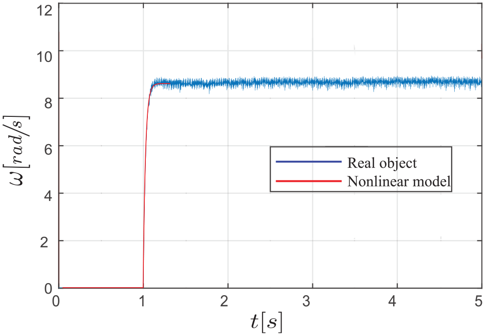
Comparison between real and nonlinear model data for step input, amplitude 5.

With the nonlinear mathematical model response of the system to the step functions of high amplitude is now good modeled. Increased amplitude does not increases the deviation of the model.

Conclusion from the Figure 7:

Figure 7.

Comparison between real and nonlinear model data for sinusoidal input, amplitude 1 and frequency 0.5 rad/s.

The response of the real object and the linear model to the sinusoidal excitation was not match well, because linear model was not following the existing nonlinearity. With the nonlinear system that is not the case. Dead zone curve is well modeled.

Conclusion from the Figure 8:

Figure 8.

Comparison between real and nonlinear model data for sinusoidal input, amplitude 5 and frequency 0.5 rad/s.

It follows that the nonlinear model quite comparable representation of the original system, for various kind of input signals.

Design of the control law

Checking the fulfillment of the conditions

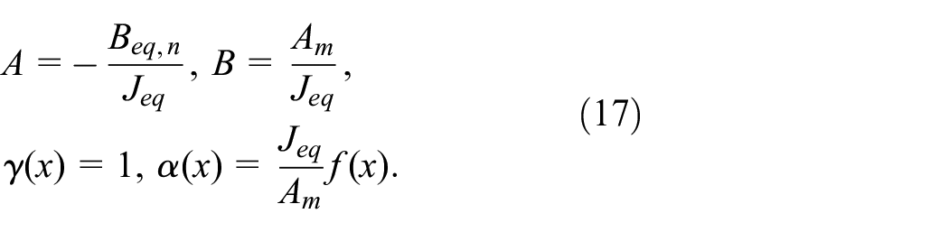
Taking into account equations (3)–(16) it could be obtained:

$$\begin{array}{c}A=-\frac{B_{\mathrm{eq},n}}{J_{\mathrm{eq}}},B=\frac{A_m}{J_{\mathrm{eq}}},\hfill \\ \gamma (x)=1,\alpha (x)=\frac{J_{\mathrm{eq}}}{A_m}f(x).\hfill \end{array}$$

(17)

• Coordinate transformation is not necessary, system is already in the suitable form for the feedback linearization;

• $\gamma (x)$ is scalar value which is different from zero;

• Pair $(A,B)$ is controllable when rank of the controllability matrix is equal to the system order;

Controllability matrix is defined as:

$$U=[B\mathrm{AB}{A}^{2}B...A^{n-1}B]$$

(18)

According to the velocity, system order is equal to $n=1$ , so controllability matrix has the form:

$$U=B=\frac{A_m}{J_{\mathrm{eq}}};$$

(19)

The number of the non-controllable states is equal to the zero.

• All functions are smooth because earlier the approximation with the differentiable tangent hyperbolic was made;

It is obvious that the condition $\mathrm{rank}U=n$ is fulfilled, so it is possible to introduce a nonlinear control that will nullify the existing nonlinearity of the system itself and perform linearization.

Control signal synthesis for the application of the feedback control method

According to the equations (4)–(17) first derivative of the output is:

$$y=x\to \stackrel{·}{y}=\stackrel{·}{x}=-\frac{B_{\mathrm{eq},n}}{J_{\mathrm{eq}}}x-f(x)+\frac{A_m}{J_{\mathrm{eq}}}u$$

(20)

As the first derivative of the output depends on the control signal the system has no internal dynamics and the relative degree of the system is equal to the order $r=n=1$ . The control that needs to be introduced to eliminate nonlinearity can be realized in different ways. In this paper it is adopted in the form:

$$u=\frac{J_{\mathrm{eq}}}{A_m}[f(x)+v]$$

(21)

The signal $v$ , that becomes the new control signal is selected as the proportional-integral PI controller:

$$v=K_p\epsilon +K_i{\int }_0^t\epsilon d\tau ,$$

(22)

where error $\epsilon =w-y$ represents the difference between the desired output variable $w$ and the real output angular velocity $y$ .

State equation linearized by feedback is:

$$\stackrel{·}{x}=-\frac{B_{\mathrm{eq},n}}{J_{\mathrm{eq}}}x+K_p\epsilon +K_i{\int }_0^t\epsilon d\tau$$

(23)

Optimization of FBC using the GWO algorithm

In this paper, for proper operation it is necessary to set the PI controller parameters and optimize them to get satisfactory dynamic behavior. Further, for the design of the optimal PI controller the metaheuristic GWO optimization algorithm was used. Moreover, the mentioned parameters are all coded into one wolf, that is one agent, that is presented with a vector which contains, in our case, two parameters. For the objective function performance criterion the integral of absolute errors (IAE) is utilized, as: $\mathrm{IAE}=\int |\epsilon |d\tau$ .

In the suggested GWO algorithm the number of the search agents is set to 30, while the maximum number of iterations is set to 500. Additionally, one agent represents one potential optimal PI controller. All of the parameter values that were used in the application of the GWO were taken from the original paper. ⁴⁵ After the optimization the obtained parameters for the scaling factors are:

$$K_p=3.8906K_i=130.0000$$

(24)

Stability check and experimental results

From the new state equation (23) and PI gains equation (24) characteristic polynomial poles of the system are easily obtained as: $p_1=-2.2261+11.1823i$ and $p_2=-2.2261-11.1823i$ . As the poles are in the left half of the s-plane the system is stable. Besides analytically, this statement is also experimentally confirmed. In the following, the comparison between the real and the desired velocity is shown.

The output and desired trajectory signals nearly match, with lightweight differences.

As it has been said, conventional control is inappropriate to struggle many problems such as steady-state error, speed changes, and load disturbances. The motion control can be tackled by mechanical or control algorithm to compensate the effect of backlash, friction, and mechanical defects. Several advance intelligent control methods for these purposes are proposed in Mao and Hung. ⁴⁷

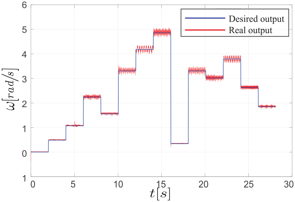
Very important references for verifying the performances of a nonlinear control system are sinusoidal signals in which the direction of rotation of the output shaft changes during operation. From the Figures 9 and 10 it can be seen that system has really fast response. Both, rising and settling time are less than $0.02s$ .

Figure 9.

Velocity tracking of step signal.

Figure 10.

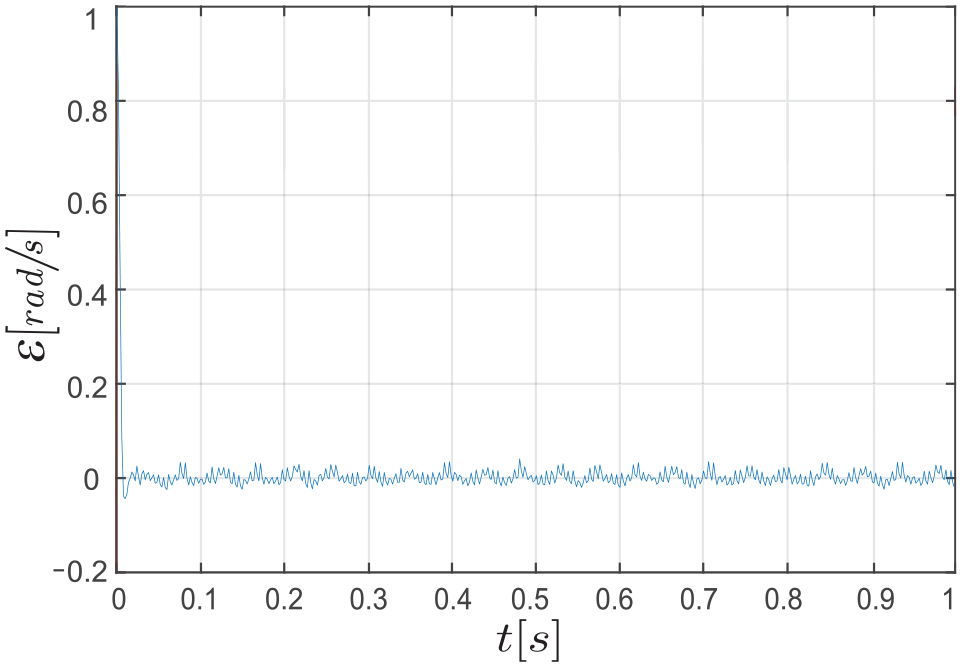
Error signal for velocity tracking of step signal.

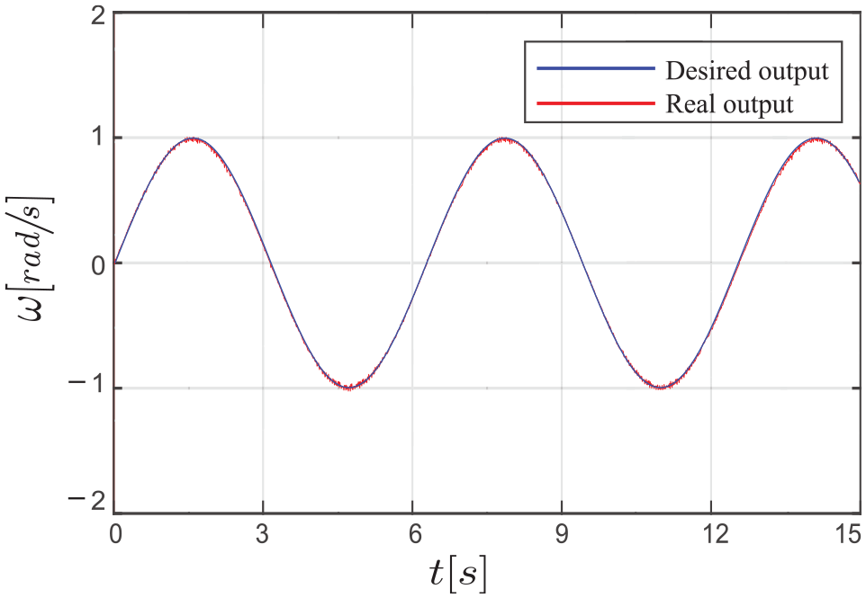
Figure 11 shows sinusoidal references for low frequency 0.1 rad/s and Figure 12 shows frequency of 1 rad/s, both with amplitude 1. Moreover, the errors of velocity tracking, are also depicted. The error for the velocity tracking is between ±0.04 rad/s, Figures 13 and 14.

Figure 11.

Velocity tracking of sinusoidal signal with small frequency of 0.1 rad/s.

Figure 12.

Velocity tracking of sinusoidal signal with frequency of 1 rad/s.

Figure 13.

Error signal for velocity tracking of sinusoidal signal with small frequency of 0.1 rad/s.

Figure 14.

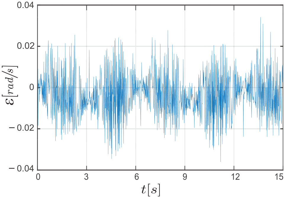
Error signal for velocity tracking of sinusoidal signal with frequency of 1 rad/s.

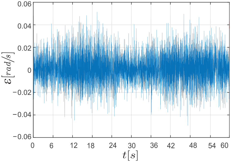
Another very useful signal for checking friction compensation in engine operation is the $\mathrm{chip}$ signal, because the frequency changes over time. In this paper authors used $\mathrm{up}-\mathrm{chirp}$ as a reference, with initial frequency od $0.1\mathrm{Hz}$ and target time $100s$ . The frequency increases linearly over time. The error is same as in sine case, Figures 15 and 16.

Figure 15.

Velocity tracking of chirp signal.

Figure 16.

Error signal for velocity tracking of chirp signal.

Furthermore, in order to test the robustness of the designed optimized FBL controller the two types of disturbances $d$ were added directly to the object, as shown in the Figure 17. Response of the system to an arbitrary excitation has been widely studied.^48–50

Figure 17.

Feedback linearization control and GWO algorithm.

The first disturbance acts continuously as band-limited white noise signal added directly to the object. Therefore, the GWO optimized coefficient of the FBL controller, have remained unchanged, and comparisons of real and desired trajectories are and given in the Figures 18 to 24. In these set of figures it could be understandably observed that errors signals are more significant in case of the applied white noise disturbance, but also that the proposed control algorithm operates effectively, although the PI coefficients are optimized for the disturbance-free case.

Figure 18.

Velocity tracking of step signal when white noise is applied as disturbance to the system.

Figure 19.

Error signal for velocity tracking of step signal when white noise is applied as disturbance to the system.

Figure 20.

Velocity tracking of sinusoidal signal with small frequency of 0.1 rad/s when white noise is applied as disturbance to the system.

Figure 21.

Error signal for velocity tracking of sinusoidal signal with small frequency of 0.1 rad/s when white noise is applied as disturbance to the system.

Figure 22.

Velocity tracking of chirp signal when white noise is applied as disturbance to the system.

Figure 23.

Error signal for velocity tracking of chirp signal when white noise is applied as disturbance to the system.

Figure 24.

Velocity tracking of selected function when white noise is applied as disturbance to the system.

The errors of velocity tracking, where disturbances are added in order to test the robustness, are given in following figures respectively: Figures 19, 21 and 23. The step signal is very important in practice especially in industry when it is necessary to maintain a constant input speed of the motor.^51,52

Here error is less than 0.06 rad/s for both sinusoidal and chirp outputs.

The second disorder acts continuously, with initial time in the $5^{\mathrm{th}}$ second of operation and is modeled as a normal step signal with final value 1. This disturbance is also simulated and applied directly to the object and it can be considered as extremely large for sinusoidal and chirp signal, because their amplitude is equal to the intensity of the disturbance.

During the operation of the system, when the given desired output signal has amplitude larger than 1, disturbance which has much less intensity does not create a huge error, Figures 25 and 26.

Figure 25.

Velocity tracking of step signal with step disturbance starting in the fifthth second.

Figure 26.

Error signal for velocity tracking of step signal with step disturbance starting in the fifth second.

On the other hand, as other references are of much lower amplitudes (sine and chirp), a disturbance of the same amplitude creates a much larger error.

However, the control system manages to quickly deal with this disturbance and the system is not derived from stability but continues to drive: Figures 27 to 30.

Figure 27.

Velocity tracking of sinusoidal signal with step disturbance starting in the fifth second.

Figure 28.

Error signal for velocity tracking of sinusoidal signal with step disturbance starting in the fifth second.

Figure 29.

Velocity tracking of chirp signal with step disturbance starting in the fifth second.

Figure 30.

Error signal for velocity tracking of chirp signal with step disturbance starting in the fifth second.

There are many ways to check the robustness of the control system. One of them is comparison of current response under varying load condition. ⁵³ In Medjghou et al. ⁵⁴ authors investigate presence of uncertainties and disturbances in object in combination with the feedback linearization control and they have concluded that FBL is unable to ensure good performances ⁵⁴ for the closed-loop system. There are many ways to overcome this problem, for example improve this control by adding a robust control term (discontinuous control). Their choice was motivated by its high robustness against uncertainties and disturbances.

Therefore, the whole control law was constituted of two terms, that is, feedback linearization control term and a discontinuous control term. This was not the case in this paper. The GWO algorithm was enough and successful even on the function of changing the desired reference very fast Figure 31.

Figure 31.

Velocity tracking of selected function with disturbance starting in the fifth second.

Conclusion

In this paper, a feedback nonlinear control system is applied to high nonlinear machine. The variable that represented the given desired response of the system is velocity of the load shaft. First, the modeling of an object is shown. After it has been experimentally confirmed that linear equations do not describe this object well enough, they have been changed. Coulomb friction was introduced, which resulted in obtaining the nonlinear mathematical model. An approximation of the part of the Stribek friction curve was made with the tangent hyperbolic function. Then, a summary of feedback linearization theory and gray wolf optimization algorithm are given. The fulfillment of the conditions for the synthesis of the control law with this approach on a given plant has been examined and proven. Some more complex systems, which use this type of engine, could also be operated on this way. Finally, using Matlab and Simulink environment, the GWO optimization algorithm was used to optimize the PI coefficient of the proposed FBL controller. Specifically, optimal PI gains for the controller were generated according to IAE performance criterion.

From the attached experimental results, with special reference to the last Section, it is easy to see that nonlinear model gives justification for the usage of the feedback linearization control technique, especially since the robustness of the control system has been tested in the case of the two types of disturbances (both of them continuously acting on the object: white noise and step signal). White noise is introduced as the way to model the random excitation. ⁵⁵ The results have shown that the proposed controller was capable of dealing with the nonlinearities of the DC motor. As the main goal of this study was to make the DC motor to track desired velocity, it is important to notice that this algorithm is convenient not only for an environments with disturbances, but also for numerous outputs. One possible area of the future work can be optimization with another metaheuristic algorithms and compare them with each other.