Sage Journals: Discover world-class research

Abstract

The dynamic characteristics of the wall lift and drag of the rigid sphere moving parallel to the single wall surface in the static viscosity laminar flow field are numerically studied, on the basis of the three-dimensional numerical simulation method of the quasi-steady “relativity of motion.” The results show that: (1) The wall surface acts to increase the drag; (2) On the near wall, the lift coefficient decreases as the Reynolds number between the sphere and the wall increase when Re < 100. However, when Re > 100, the lift coefficient increases sharply; (3) On the far wall, there is no wall effect when Re > 10, consistent with the unbounded flow, but the wall effect still exists when Re < 10; and (4) The particle rotation has few influences on drag but slightly increases the lift. And the lift induced by rotation is mainly determined by the surrounding fluid pressure. These results all contribute to the study of the hydrodynamic behavior of particles in the boundary and deepen the understanding of the phenomenon of particle transport in the wall effect layer.

Keywords

Relativity of motion wall lift force numerical investigation wall effect limited boundary

Introduction

Objects in the flow field are subjected to lateral lift perpendicular to the main flow direction, and the cause of the lift can be attributed to the asymmetry of the object or of the surrounding flow field. The lateral shift induced by lift is common in large objects such as aircraft, but the lateral migration of tiny particles is often obscured by the mixing of turbulence on a macro scale and is not appreciated.¹ The lateral migration of particles in the Poiseuille flow is originated from the experimental observation of Segré and Silberberg,² etc. They found that the neutral suspending particles in a circular tube migrated to and moved in a concentric annular position about 0.6 times the radius from the center of the pipe. It is the phenomenon of “inertial aggregation.” Subsequent studies^3–4 show that the key to lateral migration is the existence of lateral lift. When the particles migrate to a lateral position with the lift being 0, their position no longer changes and only moves in the main direction.

With deepening research in microfluidics, the phenomenon of “inertial aggregation” has attracted much attention. Combined with microfluidic chip technologies, such phenomenon has broad application prospects in areas like sewage filtration, colloid separation, cell counting, etc.^3,4 This type of device has the advantages of large output, low energy consumption, high efficiency, etc. In the literature, Huang et al.⁵ and others have made a detailed summary of its application in the industry.

Ho and Leal⁶ used the regular perturbation method to derive the lateral lift of a rigid sphere in two infinitely long plates of the Poiseuille flow, explaining that the lateral motion of the particles is caused by fluid inertia, and the lateral lift is mainly caused by two mechanisms: (1) Shear gradient lift force: The uneven shear rate gradient of the Poiseuille flow velocity distribution results in both sides of the particle being unevenly stressed and a lift in the direction of a high shear rate produced; (2) wall lift force: The presence of the wall results in the near-wall-side particles unevenly stressed and a lift in the direction of a low shear rate produced. The competition of the two lifts makes suspending particles migrate to a specific position between the center of the channel and the wall.

Di Carlo et al.⁷ numerically studied the transverse lift, using a data fitting approach to obtain approximate expressions of various components: the wall lift $F_{W} \propto ρ U^{2} a^{6} / H^{4}$ , direction away from the wall; Shear gradient lift force: in the direction away from the wall and the Shear gradient lift force: $F_{S} \propto ρ U^{2} a^{3} / H$ in the direction toward the wall. It is defined that $a$ is the particle diameter, $ρ$ the fluid density, $U$ the average fluid flow velocity, and H the characteristic length of the channel cross-section. However, these results are obtained in a smaller area and do not actually separate the two forces. The results are still highly inaccurate.

Although much progress has been made in exploring the application of “inertial aggregation” phenomenon, the mechanics of wall lift and shear gradient lift are not sufficiently explored. Cox and Hsu⁸ and Vasseur and Cox⁹ analyzed the dynamics of rigid spherical particles using the asymptotic matching expansion method of the perturbation method and obtained theoretical asymptotic solutions to the wall lift at low Reynolds numbers. However, it is within the very low Reynolds number range without relevant experimental and numerical simulation verification. Takemura and Magnaudt¹⁰ first (and to date the only known) measured the wall lift when the sphere is closer to the wall at moderate Reynolds number (Re = 1–92), but did not consider the case where the sphere was farther from the wall.

In the field of experimental and numerical studies, although the unbounded flow characteristics of spheres have been initially studied, the spheres are subject to the limiting effect of walls in the solid-liquid two-phase flow. At the same time, due to the existence of the wall surface, the wake structure and stress condition will also make a significant difference. However, due to the limitations of the current experimental measurement methods, accurate flow field information under the influence of the wall surface cannot be obtained. CFD (computational fluid dynamics) can provide this information effectively and accurately,^11–16 and it is easy to obtain flow details including the stress condition of the sphere in the flow.

In order to separate the wall lift from the shear gradient lift and eliminate the influence of shear rate on the inertia lift, a feasible way is to study the uniform linear motion of spherical particles in the static fluid near the wall.¹⁷ In this paper, based on the principle of “relative relativity of motion,” a quasi-fixed constant calculation model describing the motion of a single spherical particle under a semi-unbounded flow field is proposed.⁵ The dynamic characteristics of spherical particles under the wall effect are systematically studied using CFD technologies. Internal physical laws including the development and evolution of spherical particle wake morphology under different particle Re numbers and sphere-to-wall spacing ratios L are obtained. A research foundation is laid for further exploring the sphere motion law under the wall effect. Moreover, it is conducive to revealing the dynamic mechanism of particle motion, thus providing substantial guidance for industrial applications.

Statement of the problem and the numerical approach

Introduction to the numerical calculation model

The Reynolds number range studied in this paper is 0.5–250. The research object is a rigid sphere suspending in the liquid phase and moving parallel to the bottom wall in a steady uniform linear motion with a velocity of −u in a stationary fluid. The flow is essentially a liquid-solid two-phase flow with a single particle, but the present two-phase flow numerical method contains many empirical parameters to be artificially set, with great approximation and uncertainty. Therefore, this paper does not intend to deal with this problem by using the conventional two-phase flow numerical calculation method, but directly considers the sphere surface as a moving solid boundary of the flow field. Thus, the flow field studied is a laminar flow with a sphere digged out as shown in Figure 1. Therefore, it is translated into a conventional single-phase flow problem.

Figure 1.

Schematic diagram of a sphere moving parallel to a wall in a stationary fluid.

In the unbounded uniform flow, Johnson and Patel.¹⁸ have determined that the wake behind the sphere remains stable and a steady-state steady flow when Re < 270 while unstable, when Re = 280, it indicates that the critical Reynolds number 270–280 changes. In unbounded uniform flow, Johnson et al.¹⁸ have determined that the sphere behind the wake remains stable at Re < 270, a steady-state constant flow, and becomes non-stationary flow at Re = 280, indicating that the Reynolds number changes at some value between 270 and 280. Zeng et al.¹⁹ studied that the existence of the wall surface inhibits the detachment of the vortex, thereby delaying the occurrence of the unsteady flow. Therefore, it is a constant flow in the range of Reynolds number studied in this paper, and the steady calculation is reliable in the relative motion model.

If the stationary absolute coordinate system (such as the O-XYZ coordinate system shown in Figure 1) is used as the reference frame, this flow field is an unsteady flow field. When performing calculations under this model, a lot of time will be consumed because of its complication with techniques such as dynamic meshing and time advancement being required. If the coordinate system used in the CFD calculation is fixed to the sphere center and translates at the same speed as the sphere does (such as the o-xyz coordinate system shown in Figure 1). In this translational coordinate system: the translational velocity of the sphere is zero, and the wall and flow fields are transformed into a uniform linear motion with the velocity being U so that the calculation model becomes a constant flow field. The motion coordinate system is essentially an inertial system. As long as the boundary condition is changed, the existing CFD code can be still used directly. All above provide convenience for the numerical study of this paper.

Related physical parameters

The computational model uses a three-dimensional, steady, incompressible N-S (Navier-Stokes) equation, and the control equation is as follows:

{\begin{matrix} \nabla \cdot u = 0, \\ (u \cdot \nabla) u = - \frac{1}{ρ} \nabla p + υ \nabla^{2} u . \end{matrix}

(1)

Where $p$ is the fluid pressure; $ρ$ , $υ$ is the fluid density and kinematic viscosity, both constant (incompressible fluid); $u$ is the velocity in the translational coordinate system.

The proportional distance between the center of the sphere and the wall L:

L = \frac{l}{D},

(2)

Where $l$ is the distance from the sphere center to the wall; D is the sphere diameter.

Particle Reynolds number:

Re = \frac{UD}{υ},

(3)

Where: $U$ is the speed of the sphere.

Define the z = 0, y = 0 plane dimensionless vortex as:

{Ω_{z}}^{*} = (\frac{\partial v}{\partial x} - \frac{\partial u}{\partial y}) \cdot D / U,

(4)

{Ω_{y}}^{*} = (\frac{\partial u}{\partial z} - \frac{\partial w}{\partial x}) \cdot D / U,

(5)

The dimensionless distance L* of the sphere from the wall:

L^{*} = \frac{Ul}{υ} = LRe .

(6)

Resistance and lift are the two components of the force acting on the sphere, namely the X-axis direction of the translational motion and the normal Y-axis direction of the wall, calculated by integrating the pressure and viscous stress on the sphere surface.

F_{D} = F_{D, p} + F_{D, τ} = e_{x} \cdot (\int_{S} - p e_{n} d S + \int_{S} e_{n} \cdot [τ] d S),

(7)

F_{L} = F_{L, p} + F_{L, τ} = e_{y} \cdot (\int_{S} - p e_{n} d S + \int_{S} e_{n} \cdot [τ] d S) .

(8)

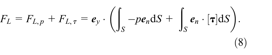
Where: $S$ – spherical surface area; [ $τ$ ] – viscous stress tensor; $e_{x}$ and $e_{y}$ are unit vectors in x and y directions, respectively; the former of the above two equations is the pressure term, and the second is the viscosity term.

The non-dimensionalization of the above equations is available as follows:

C_{D} = C_{D, p} + C_{D, τ} = \frac{F_{D, p} + F_{D, τ}}{1 / 8 π ρ U^{2} D^{2}},

(9)

C_{L} = C_{L, p} + C_{L, τ} = \frac{F_{L, p} + F_{L, τ}}{1 / 8 π ρ U^{2} D^{2}} .

(10)

Where $C_{L, p}$ and $C_{L, τ}$ are the pressure lift coefficient and the viscosity lift coefficient.

Discussion of grid independence

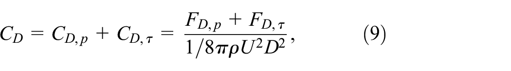
In the CFD calculation of this paper, the flow field calculation domain is divided by a hybrid grid, in which the local grid refinement is performed near the sphere and in the wake region to improve the accuracy, as shown in Figure 2. The grid density affects not only the calculation accuracy but also the efficiency. In order to eliminate the possible impacts of grid quality on the calculation results, this paper verifies the grid independence. The grid convergence analysis takes the sphere motion condition of L = 1 and Re = 10 as an example, and three kinds of grids from the sparse to the dense are selected for simulation calculation. The results are shown in Table 1.

Figure 2.

Schematic diagram of meshing.

Table 1.

Grid convergence analysis.

Case	Grids	C_D	C_L
GI	251,500	4.719	0.345
GII	502,800	4.723	0.353
GIII	998,000	4.725	0.356
Zeng et al.¹⁹	–	4.721	0.351
Sugioka and Tsukada²⁰	–	4.727	0.355

Table 1 gives the data comparison of the drag coefficient C_D, wall lift coefficient C_L of this paper that and those of Zeng et al.,¹⁹ Sugioka and Tsukada²⁰ under three sets of grids. The results all have high goodness of fit. It is not difficult to find that the difference between C_D and C_L caused by different grid numbers is small. A further comparison shows that the results of standard grid GII and fine grid GIII are very close, while there is a slight gap between the results of coarse grid GI and those of the other two sets. By comparing the standard grid GII with the data in Zeng et al.¹⁹ and Sugioka and Tsukada,²⁰ the maximum error among drag coefficients is 0.08%, and the maximum error among the lift coefficients is 0.5%. Therefore, the grid GII is selected for the further study, comprehensively considering the computational cost and efficiency.

Computational domain verification

To ensure the computational accuracy of the numerical simulation, the computational domain-independence verification must be performed. Using three different sets of computational domains under grid GII, the computational conditions are L = 1 and Re = 10. As seen in Table 2, the results remain constant under the three sets Therefore, the computational domain of 60D × 60D × 300D is adopted.

Table 2.

Computational domain independence analysis.

Computational domain size	C_D	C_L
40D × 40D × 200D	4.724	0.356
60D × 60D × 300D	4.723	0.353
80D × 80D × 400D	4.723	0.354

Numerical algorithm

The software used for the numerical simulation is ANSYS-FLUENT. The coupling of pressure and velocity of the N-S equation adopts the “SIMPLEC” algorithm in the solving process; the convection term is discretized by the third-order precision “QUICK format”; the viscous term is discretized by the “central format” with second-order precision.

Boundary conditions: The sphere is located in the middle of the computational domain, and only the Y-axis position of the sphere center is changed; The boundary condition on the left side of the computational domain is set as the velocity inlet, and that on the right side is set as the pressure outlet; The bottom wall adjacent to the sphere is set as the no-slip wall surface, and the remaining three surfaces are set as the far-field conditions, which means that the normal gradient of the flow velocity on these three surfaces is zero.

Results and discussions

Drag force

Regarding the unbounded flow of the sphere with $Re \leq 250$ , many scholars have carried out a lot of research on the drag coefficient C_D. When Re is small, the resistance coefficient of a sphere is commonly calculated by Schiller and Naumann’s empirical formula²¹:

C_{D} = \frac{24}{Re} (1 + 0.15 R e^{0.687}) .

(11)

In this paper, we first compare the simulated unbounded flow drag coefficient with the equation from the literature²¹ (Figure 3). From the figure, it can be seen that the two agree well within the range of Re numbers calculated in this paper.

Figure 3.

Comparison of numerical calculation results with the results of the literature²¹ empirical formula.

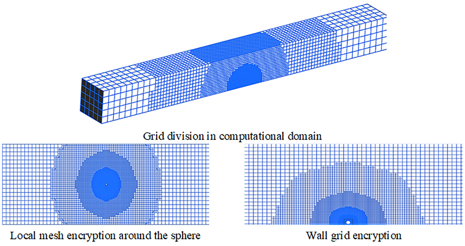
Figure 4 is a distribution diagram of the drag coefficient C_D changing with the Reynolds number changing at different distances L between the sphere and the bottom wall. Figure 4 shows that the sphere drag coefficient at different L and the distribution of unbounded flow drag coefficient share a similar trend. Within the entire Re number range studied, the drag coefficient of the sphere decreases as the L value increases. When Re < 100, the closer the distance from the wall is, the higher the drag coefficient is, all higher than that of the unbounded flow. When Re > 100, the closer the distance from the wall (such as L = 0.75) is, the higher the drag coefficient is. But when the distance from the wall is far, the drag coefficient is slightly lower than that of the unbounded flow.

Figure 4.

Relationship between drag coefficient and Re number under different working conditions.

Kim et al.²² studied the case where a pair of spheres were juxtaposed at a fixed speed in a stationary fluid. It is observed that the drag coefficient increases as the two spheres approach each other. When the distance between the two spheres slightly increases, the drag coefficient is slightly lower than the asymptotic value of a single isolated sphere. Due to the existence of the wall, the slight decrease in the drag coefficient at the higher Re number appears to be very special. This phenomenon was also observed in the asymptotic results of the low Reynolds number of Vasseur and Cox,⁹ who explained the result in detail from the perspective of the potential flow.

Oseen flow approximate resistance coefficient formula:

C_{D, free} = \frac{24}{Re} (1 + \frac{3}{16} Re),

(12)

When the sphere is closer to the wall, namely Re << L* << 1, Vasseur and Cox⁹ derived an asymptotic equation with an increase of drag coefficient:

C_{D} - C_{D, free} = \frac{27}{4 L^{*}},

(13)

As the distance between the sphere and the wall increases, namely Re << 1 << L*, a progressive equation with a reduced drag coefficient is obtained:

C_{D} - C_{D, free} = - \frac{9 β}{2 {(L^{*})}^{5 / 2}}, β = 0.50698 .

(14)

The calculation results in this paper are consistent with the above-mentioned low Reynolds number prediction, and the resistance coefficient of each working condition is plotted as a functional form of (C_D–C_D, free) L* and L* relationship, as shown in Figure 5. The numerical results fit well into a straight line in the form y = aL* + b, where the slope a is −3.877 and the intercept b is 47.641. In this paper, the fitting expression of the drag coefficient of the sphere motion under the wall effect is as follows:

C_{D} = \frac{24}{Re} (1 + \frac{3}{16} Re) - 3.877 + \frac{47.641}{L^{*}} .

(15)

Figure 5.

Fitting of the drag coefficients of L = 0.75–12.

The drag coefficient formula proposed in this paper has a wider range of Reynolds numbers than Vasseur and Cox’s theoretical formulas (13) and (14) do and is more in line with actual calculation needs. The Vasseur and Cox resistance formula is a piecewise function. The formula of this paper concludes various conditions with a wider application scope.

Research on the near-wall lift

This paper first studies the unbounded flow of a sphere, as shown in Figure 6. When Re = 2, 10, the flow structure takes on an attached flow, symmetrical before and after and above and below the sphere, and there is no significant difference. When 20 < Re < 210, the flow becomes constant, separated, and axisymmetric. The topology is similar. The three-dimensional structure at this time is a vortex ring behind the sphere. The results of this paper agree well with those of Johnson and Patel.¹⁸

Figure 6.

Flow structure behind sphere in unbounded flow: (a) L = ∞ and Re = 2, (b) L = ∞ and Re = 10, (c) L = ∞ and Re = 100, and (d) L = ∞ and Re = 200.

Figure 7 is a flow line flow structure distribution around the surface of the sphere when z = 0 for L = 0.75 and L = 2. The existence of the wall breaks the axial symmetry of the flow around the sphere, which is observable at all Re numbers of L = 0.75. As the distance between the sphere and the wall increases, the streamline and the vorticity contours asymmetry becomes weak when L = 2, but it can still be observed. At lower Re numbers, the flow structure around the sphere remains unchanged. Due to the wall effect, the front and rear stagnation points move down and toward the wall surface compared with the unbounded flow. When Re = 200, a recirculation zone can be seen in the wake. However, unlike the unbounded flow, the wake structure takes on significant asymmetry when L = 0.75. When L = 2, the asymmetry is insignificant.

Figure 7.

Streamline flow structure around the sphere at z = 0: (a) L = 0.75 and Re = 2, (b) L = 0.75 and Re = 10, (c) L = 0.75 and Re = 200, and (d) L = 2 and Re = 200.

Vasseur et al.⁹ used the asymptotic matching expansion in the singular-perturbation method, deriving the wall lift of a sphere moving at a constant velocity in a stationary viscous fluid at low Re numbers. It is found that the lift coefficient C_L is only a function of L*, as shown in equation (16):

C_{L} = {\begin{matrix} \frac{9}{8} (1 - \frac{11}{32} {L^{*}}^{2}), L^{*} << 1, \\ \frac{9}{2} \cdot {{(L^{*})}^{- 2} + 2.21901 {(L^{*})}^{- \frac{5}{2}}}, L^{*} >> 1, \end{matrix}

(16)

Takemura and Magnaudet¹⁰ used optical techniques to study the clean and contaminated (similar to rigid spheres) bubbles moving parallel to the wall in a stationary fluid. The results show that the lift coefficient C_L is a function of L* and Re (or L and Re). The experimental results of wall lift are fitted by the following formula:

C_{L} = C_{L 0} a^{2} {(L / 1.5)}^{- 2 \tanh (0.01 Re)},

(17)

a = 1 + 0.6 R e^{1 / 2} - 0.55 R e^{0.08},

(18)

C_{L 0} = {\begin{matrix} (9 / 8 + 5.78 \times 10^{- 6} L^{* 4.58}) \exp (- 0.292 L^{*}), 0 < L^{*} < 10, \\ 8.94 L^{* - 2.09}, 10 \leq L^{*} < 300 . \end{matrix}

(19)

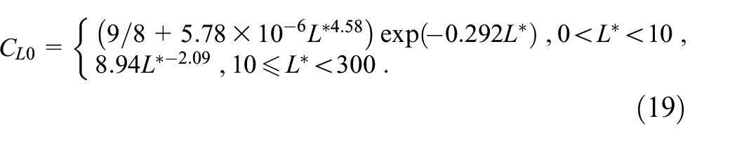
For ease of comparison, Vasseur and Cox’s low Reynolds number progressive theory results (equation (16)) and lift formula models derived by Takemura and Magnaudet (equations (17)–(19)) are plotted in Figure 8 along with the lift coefficient distributions calculated herein. The figure shows that the results of this paper are consistent with those of Vasseur and Cox under the smaller L*. When L = 0.75, and L = 1, when L*< 100, the results of this paper are consistent with the Takemura and Magnaudet model formula. When L = 2 and L = 4, the result consistency range is within L*< 200. When L* is larger the lift coefficients of equations (17)–(19) will be lower one order of magnitude than the numerical results herein. This is because the Re numbers studied by Takemura and Magnaudet are only in the range of 1–92, within which the experiment is in good agreement with the simulation results.

Figure 8.

Results comparisons.

Figure 9 shows the distribution relationship between the lift coefficient C_L and the dimensionless distance L* calculated in this paper. The dashed connection is expressed as the same Reynolds number. The lower Reynolds number-theoretical asymptotic curve by Vasseur and Cox⁹ is also shown. When L* is smaller (or smaller Re numbers), the lift coefficient C_L calculated in this paper is very consistent with the progressive results predicted by Vasseur and Cox’s low Reynolds number theory. As the L* increases, the lift coefficient initially drops rapidly, but the decline rate is always lower than the theoretically predicted asymptotic value. As the Re number increases further and L remains constant, C_L does not monotonically decrease with the increase of L* and increases rapidly after reaching a certain L* value. Figure 9 shows that this turning point occurs when Re is within 100–200. However, although the lift coefficient takes on such a significant increase the lift coefficient is still an order of magnitude smaller than the theoretical lift coefficient C_L = 9/8 at the limit L* → 0 in the range of Reynolds numbers studied in this paper.

Figure 9.

Wall lift coefficient C_L and L* relationship diagram.

To more clearly compare the contribution characteristics of each part of the wall lift coefficient C_L, Figure 10 shows the relationship of the lift coefficient C_L with its pressure lift coefficient C_LP and the viscous lift coefficient C_Lτ and L when the working conditions L = 1, and L = 2 at different Reynolds numbers (The results for other operating conditions are similar and therefore are not plotted). When L* is smaller, the main contribution of wall lift is from the viscosity term, and when L* is larger (correspondingly higher Re number), its main contribution comes from the pressure term. The pressure lift coefficient distribution is consistent with the trend of the viscous lift distribution.

Figure 10.

The composition of the wall lift on the sphere.

Figure 11 shows the distribution of pressure coefficients when L = 1 at each Re number in the z = 0 surface of the sphere, where C_P = (p − p ∞)/(0.5 ρ U²). If there is no wall surface, the pressure distribution on the upper and lower surfaces is coincident, and there is no difference between the upper and lower surfaces. It can be seen from the figure that when Re < 100, the pressure of the lower surface of the sphere is first greater and then smaller than that of the upper surface as the arc length increases. The asymmetry effect caused by the wall surface gradually decreases with the increase of the Re number. When the Re number is further increased to 200, the pressure of the lower surface of the sphere is greater than that of the upper surface under all arc lengths. A slight change will contribute to the increase of the wall lift.

Figure 11.

Distribution of pressure coefficients around the sphere at z = 0: (a) L = 1 and Re = 2, (b) L = 1 and Re = 10, (c) L = 1 and Re = 100, and (d) L = 1 and Re = 200.

Exploring the wall lift at a distance

As can be seen from Figure 12, the lift coefficient of the sphere in the farther area will rapidly decrease with the increase of Re number and become zero when Re = 10. The sudden drop in the lift coefficient at low Re numbers is consistent with the near-wall lift trend, absolutely a mechanism induced by the wall. This mechanism shows that the wall is more restrictive at low Re numbers. Re = 10 is a turning point with a lift coefficient being zero at a distance. When the L value increases, the wall lift of the sphere at the same Re number will decrease.

Figure 12.

Lift coefficients when Re < 30.

When the sphere is far from the bottom wall, it still has a small lift coefficient when Re < 10. This paper combines the calculation results with the low Reynolds number theory by Vasseur and Cox.⁹ As shown in Figure 13, it is found that as the value of L becomes larger, the lift coefficient variation curve is closer to the theoretical asymptotic curve predicted by Vasseur et al. The premise of Vasseur and Cox’s prediction is that: L >> 1. This is good support for the calculation results of this paper. When the L value studied in this paper is larger, the lift coefficient curve by simulated calculation will be closer to the theoretical prediction by Vasseur and Cox.

Figure 13.

Lift coefficient and L* at various working conditions.

When Re > 10, the sphere is almost free from wall action. When10 < Re < 210, the lift coefficient C_L is about zero, consistent with the unbounded flow. Figure 14 shows the variation trend of lift coefficients under different conditions where Re are within 210–250.The corresponding results by Johnson and Patel¹⁸ for the unbounded bypass study are also plotted for comparison. When L = 6, 8, 12, the variation trend is consistent with that of the unbounded flow lift coefficient. In addition, the numerical calculation results of this paper are consistent with those of Johnson and Patel.¹⁸ At higher Reynolds numbers L = 6, 8, 12 (Re > 10), it can be assumed that the wall surface has no lifting effect on the sphere. However, when Re < 10, the lifting force of the wall surface on the sphere still exists, which shows that the lifting effect of the wall surface on the sphere still exists at low Reynolds, at least with stronger limitation than it does at higher Reynolds.

Figure 14.

Lift coefficient of each working condition when Re = 210–250.

Figure 15 is a streamline flow structure diagram of each cross-section of the sphere when L = 6 and Re = 250, consistent with the unbounded flow. Figure 15(b) and (d) show the sphere surface y = 0 when Re = 250, the flow structure on which is symmetrical. It can also be seen from Figure 15(a) and (c) that behind the sphere is no longer a vortex ring at this time. When L = 6, 8, 12, the calculation results o in this paper are in good agreement with the visualization results of by unbounded flow around of Johnson and Patel¹⁸ when Re = 210–250.

Figure 15.

Streamline flow structure diagram at Re = 250: (a) L = 6 and z = 0, (b) L = 6 and y = 0, (c) L = ∞ and z = 0, and(d) L = ∞ and y = 0.

The effect of rotation on lift and drag

In the working conditions above, the sphere moves in a uniform linear motion parallel to the bottom wall, but the sphere rotation is not considered. In the actual situation, the asymmetry of the nearby flow field caused by the wall surface (which causes lift) will inevitably induce the sphere rotation. This section takes the sphere rotation into account and explores the impacts of the sphere rotation on the lift and drag forces. It is expected to explore the lift proportion generated by the sphere rotation from a quantitative perspective. The “no-rotation” case is considered first, followed by the passive sphere rotation induced by the surrounding asymmetric flow field. The rotation angular speed of the sphere with the sphere torque being zero is the stable rotation speed. By comparing the force characteristics of the sphere in the above two cases, the degree of rotation influence on the wall lift and drag is explored.

Figure 16 is a graph showing the distribution of drag coefficients when the L = 1 sphere has no rotation or takes on stable rotation. Within the entire Reynolds number range of the study, the effect of rotation on-drag is tiny, almost making no difference.

Figure 16.

Distribution of drag coefficients of a sphere with no rotation and stable rotation when L = 1.

Figure 17 is a graph showing the distribution of lift coefficients when the L = 1 sphere has no rotation or takes on stable rotation. When Re << 1, the results by Saffman²³ show that in the unbounded linear shear flow, the lift caused by rotation is much smaller than that caused by shear. The results of this study show a similar behavior: when Re << 1, the lift caused by rotation is much smaller than that by wall induction. As shown in Figure 17, when Re > 100, the rotation has a certain influence on the lift magnitude, slightly increasing the lift coefficient. The total lift coefficient is further decomposed into a pressure lift coefficient C_LP and a viscosity viscous lift coefficient C_Lτ, and the results show that the main effect of the rotation comes from the pressure term.

Figure 17.

Lift coefficient of t no rotating and rotating spheres when L = 1.

Bagchi and Balachandr²⁴ studied the effect of rotation on drag and lift in an unbounded linear shear flow, and concluded that the net lift on a rotating sphere can be attributed to the “Magnus lift effect.” The difference between the lift coefficient with rotation considered into account and that without rotation considered into account can be expressed as Magnus lift coefficient:

C_{L, Mg} (Re, Ω_{st}) = C_{L} (Re, Ω_{st}) - C_{L} (Re, Ω_{st} = 0) .

(20)

Rubinow and Keller²⁵ derived the Magnus lift expression of the rotating sphere in the simple shear flow of Re < 1:

C_{L, Mg} = Ω d / | U | .

(21)

Where: Ω is the angular velocity of the sphere rotation, and U is the relative velocity between the sphere and the surrounding fluid.

The ratio obtained under the wall effect is about 0.5–0.65, consistent with those by Bagchi and Balachandar.²⁴ They observed a ratio of about 0.55 in the unbounded linear shear flow. Oesterle et al.²⁶ and Tanaka et al.²⁷ observed experimentally the ratios of 0.4–0.25, respectively. The difference between the results and experiments in this paper can be attributed to the wall effect. However, these results can all indicate that the contribution of the Magnus effect to lift is linearly proportional to $Ω_{st} d / | U |$ (Figure 18).

Figure 18.

Magnus lift coefficients calculated by ratio.

Conclusions

In this paper, the mechanical properties of a rigid circular sphere in a uniform linear motion under wall effect along the direction parallel to the wall are systematically studied, and the following conclusions are obtained:

When the distance between the sphere and the wall is close (L = 0.75), the role of the wall is to increase the resistance. When the distance between the sphere and the wall is a little farther (L > 1), the wall action leads to a slightly decreased drag coefficient lower than that of unbounded bypass. In this paper, we obtain the expression of the drag coefficient for the sphere motion under the wall effect.

C_{D} = \frac{24}{Re} (1 + \frac{3}{16} Re) - 3.877 + \frac{47.641}{L^{*}} .

When the sphere is near the wall (L = 0.75, 1, 2, 4), the wall lift coefficient C_L decreases with the Reynolds number and the distance between the sphere and the wall increasing for Re < 100. However, when Re > 100, the lift coefficient increases sharply with the increase of Re number. The increase of lift is also reflected in the pressure and viscosity terms, respectively.

When the sphere is far from the wall (L = 6, 8, 12), the lift mechanism is not equivalent to that near the wall, and the effect of lift is mainly concentrated on the low Reynolds number (Re < 10). When Re > 10, the lifting effect of the wall on the sphere no longer exists.

Rotation exerts insignificant effects on drag, but can slightly increase the lift coefficient. Moreover, the main effect of rotation comes from the pressure term. The lift generated by sphere rotation is called the “Magnus effect,” with its Magnus lift coefficient ratio being about 0.5–0.65.

These findings all contribute to deepening the understanding of particle transport phenomena in wall-effect laminar flow fields and promote the application of inertial microfluidic devices in the industry.

Footnotes

Handling Editor: Chenhui Liang

Author contributions

He Zou wrote the paper and made the numerical investigations; Qikun Wang helped to analyze the numerical data and paper revisions; Zhuangzhuang Xue provided indispensable support for this research and paper revisions.

Declaration of conflicting interests

The author(s) declared no potential conflicts of interest with respect to the research, authorship, and/or publication of this article.

Funding

The author(s) disclosed receipt of the following financial support for the research, authorship, and/or publication of this article: This work was supported by the National Natural Science Foundation of China (Grant No. 51776128).

ORCID iD

He Zou

References

Amini

Lee

Di Carlo

Inertial microfluidic physics. Lab Chip 2014; 14: 2739–2761.

Silberberg

Segré

Radial particle displacements in Poiseuille flow of suspensions. Nature 1961; 4760: 209–210.

Asmolov

Dubov

Nizkaya

, et al. Inertial focusing of finite-size particles in microchannels. J Fluid Mech 2018; 840: 613–630.

Hood

Lee

Roper

Inertial migration of a rigid sphere in three-dimensional Poiseuille flow. J Fluid Mech 2015; 765: 452–479.

Huang

Man

Jiang

, et al. Inertial microfluidics: recent advances. Electrophoresis 2020; 41: 2166–2187.

Leal

LG.

Inertial migration of rigid spheres in two-dimensional unidirectional flows. J Fluid Mech 1974; 65: 365–400.

DiCarlo

Edd

Humphry

, et al. Particle segregation and dynamics in confined flows. Phys Rev Lett 2009; 102: 94503.

Cox

Hsu

SK.

The lateral migration of solid particles in a laminar flow near a plane. Int J Multiphase Flow 1977; 3: 201–222.

Vasseur

Cox

RG.

The lateral migration of spherical particles sedimenting in a stagnant bounded fluid. J Fluid Mech 1977; 80: 561–591.

10.

Takemura

Magnaudt

The transverse force on clean and contaminated bubbles rising near a vertical wall at moderate Reynolds number. J Fluid Mech 2003; 495: 235–253.

11.

Belhocine

Numerical study of heat transfer in fully developed laminar flow inside a circular tube. Int J Adv Manuf Technol 2016; 85: 2681–2692.

12.

Belhocine

Abdullah

OI.

Numerical simulation of thermally developing turbulent flow through a cylindrical tube. Int J Adv Manuf Technol 2019; 102: 2001–2012.

13.

Belhocine

Wan Omar

WZ.

Analytical solution and numerical simulation of the generalized Levèque equation to predict the thermal boundary layer. Math Comput Simul 2021; 180: 43–60.

14.

Belhocine

Wan Omar

WZ.

Computational fluid dynamics (CFD) analysis and numerical aerodynamic investigations of automotive disc brake rotor. Int J Interact Des Manuf 2018; 12: 421–437.

15.

Alam

Tunc

An analytical method for solving exact solutions of the nonlinear Bogoyavlenskii equation and the nonlinear diffusive predator–prey system. Alexandria Eng J 2016; 55: 1855–1865.

16.

Belhocine

Omar

WZW

. Numerical study of heat convective mass transfer in a fully developed laminar flow with constant wall temperature. Case Stud Therm Eng 2015; 6: 116–127.

17.

Zhang

Yan

Yuan

, et al. Fundamentals and applications of inertial microfluidics: a review. Lab Chip 2016; 1: 10–34.

18.

Johnson

Patel

VC.

Flow past a sphere up to a Reynolds number of 300. J Fluid Mech 1999; 378: 19–70.

19.

Zeng

Balachandar

Fischer

Wall-induced forces on a rigid sphere at finite Reynolds number. J Fluid Mech 2005; 536: 1–25.

20.

Sugioka

Tsukada

Direct numerical simulations of drag and lift forces acting on a spherical bubble near a plane wall. Int J Multiphase Flow 2015; 71: 32–37.

21.

Schiller

A drag coefficient correlation. Zeit Ver Deutsch Ing 1933; 77: 318–320.

22.

Kim

Elghobashi

Sirignano

WA.

Three-dimensional flow over two spheres placed side by side. J. Fluid Mech 1993; 246: 465–488.

23.

Saffman

PG.

The lift on a small sphere in a slow shear flow. J Fluid Mech 1965; 22: 385–400.

24.

Bagchi

Balachandar

Effect of free rotation on the motion of a solid sphere in linear shear flow at moderate Re. Phys Fluids 2002; 14: 2719–2737.

25.

Rubinow

Keller

JB.

The transverse force on a spinning sphere moving in a viscous fluid. J Fluid Mech 1961; 11: 447–459.

26.

Oesterle

Tri

Vial

JL.

Measurements of lift and torque on a rotating sphere at intermediate Reynolds numbers. Mech Res Commun 1991; 2–3: 145–150.

27.

Tanaka

Yamagata

Tsuji

. Experiment of fluid forces on a rotating Experiment of fluid forces on a rotating sphere and spheroid. In: KSME/JSME thermal and fluid engineering conference, Jeju Island, Korea, 1990, pp.366–369.

Characteristics of lift and resistance of spherical wall in semi-unbounded flow field

Abstract

Keywords

Introduction

Statement of the problem and the numerical approach

Introduction to the numerical calculation model

Related physical parameters

Discussion of grid independence

Computational domain verification

Numerical algorithm

Results and discussions

Drag force

Research on the near-wall lift

Exploring the wall lift at a distance

The effect of rotation on lift and drag

Conclusions

Footnotes

Author contributions

Declaration of conflicting interests

Funding

ORCID iD

References