Sage Journals: Discover world-class research

Abstract

The blade outlet angle, wrap angle, and number of blades of the impeller are optimized to increase the pumping efficiency of the automotive coolant pump while keeping the size constant. Three new variants were designed and the optimal one was selected for the comparison with the original scheme. The experiment was conducted to test the hydraulic performance of the optimized impeller. The results show that the energy characteristics of the optimized impeller are in reasonable agreement with the experimental data. The energy characteristics and internal flow details of original scheme and optimized scheme are analyzed and compared. It was found that increasing the wrap angle while decreasing blade outlet angle appropriately can improve the flow conditions and the pressure distribution in the impeller and the volute, especially at low flow rates. At the designed flow rate, increasing the wrap angle while decreasing the number of blades and blade outlet angle can significantly increase the efficiency of the pump. And the maximum efficiency of the optimized impeller is 4.8% higher than the efficiency of the original impeller. The results of the study can guide designers in optimizing an automotive centrifugal coolant pump and reduce energy consumption of the automotive cooling system.

Keywords

Automotive coolant pump optimization wrap angle blade number blade outlet angle

Introduction

The automotive coolant pump is a central component of the engine cooling system. It provides circulation of the coolant flow in the piping to ensure the normal operation of the engine.¹ Due to limited installation space, radial distance of automotive coolant pump impeller is limited. In order to meet the requirements of the head, the rotational speed is high. Therefore, the automotive coolant pump not only needs to cool other parts of the engine but also needs to cool its own drive motor. A complex flow channel is needed to convey coolant to the rotor area of the motor and then convey it back to the inlet. Compared with standard centrifugal pump, the automotive coolant water pump is smaller in size and more complex in runner because of limited installation space, which often results in low efficiency. According to the different drive systems, the automotive coolant pumps are driven mechanically or electrically.² Electrically driven water pumps are increasingly used due to their relatively higher energy efficiency.^3–5

Many interesting studies have been conducted to investigate and optimize the performance of standard centrifugal pumps.^6–9 Wang et al.¹⁰ numerically optimized the impeller based on the Latin Hypercube method and found that the efficiency of the optimized pump is improved, and the vibration intensity is attenuated. Zhang et al.¹¹ investigated the effects of modifying the blade pressure side (EPS profile) on unsteady pressure pulsations and flow structures in a low specific speed centrifugal pump using experimental and numerical methods and found that the newly introduced EPS profile helps to reduce pressure pulsations and improves the uniformity of the flow field in the blade trailing edge region.

With the rapid development of the automotive industry, progress has also been made in the research of automotive coolant pumps. Researchers mainly conduct the analysis of hydraulic performance and its heat dissipation performance in the cooling system.^12–14 Li¹⁵ established a hydraulic loss model for each section of the automotive coolant pump and determined a relationship among the loss coefficient, Reynolds number, and the specific speed. Liu¹⁶ investigated the hydraulic performance of the automotive coolant pump at different speeds and then proposed a velocity control scheme for vehicle start-up. Bai¹⁷ performed the spiral optimization at the volute tongue to reduce the cavitation intensity. Li¹⁸ developed a modified cavitation model to investigate the effect of temperature on the operation of the automotive coolant pump. The results showed that the cavitation performance was worse at high temperature. Wickerath et al.¹⁹ designed an adjustable guide vane to control the coolant flow and reduce the noise of the coolant pump.

Many studies have been conducted to optimize standard centrifugal pumps, but multi-factor multi-level orthogonal optimization method was often used, and the workload was too great. The automotive coolant pump is small in size, high in rotation speed, and the flow channel of the pump chamber is relatively more complex, so the optimization results of standard pumps cannot be directly used for automotive coolant pumps. There are also many reports on the automotive coolant pumps with high rotational frequency and small size, but few of them focus on hydraulic performance.

Automotive coolant pumps are most often designed as centrifugal pumps, where the impeller is the core component and directly affects the performance of the whole system. In order to reduce energy consumption and improve the operating efficiency of the automotive coolant pump, the impeller was reshaped on the premise of unchanged outer dimensions. The energy performance and pressure pulsations of the different variants were investigated using CFD and compared in this paper. The research results can serve as a reference to automotive pump designers in the optimization process of a centrifugal coolant pump, so as to improve the operating efficiency and reduce energy consumption of the automotive pump.

Computation model and research method

Computation model

The design parameters of automotive coolant pump are as follows: flow rate Q_d = 12 m³/h, head H_d = 20 m, rotational speed n = 6000 r/min, specific speed n_s = 133.

According to the relative velocity distribution in the original impeller obtained by numerical simulation, it is obvious that the blade outlet angle is too large and the flow diffusion between blades is serious. There the blade outlet angle is reduced to 30° from 40°, according to the scope of wake area at impeller outlet. (In order to facilitate the comparison of different schemes and considering the structure of the paper, the relative velocity distribution in the original impeller is presented in Figure 10.)

The number of blades of the original impeller is high, resulting in unnecessary blocking of the flow cross-section and an increase in the contact area between the liquid flow and the walls. Both phenomena cause excessive hydraulic loss, resulting in a reduction in efficiency. According to theoretical head calculation formula of finite number of blades, the head can be more than 20 m when the blade number is reduced to 6, however, the head is less than 20 m, when the blade number is reduced to 5. Therefore, the number of blades is selected as 6.

On the other hand, a reduction in the number of blades can lead to the occurrence of the secondary flows. To ensure stable flow in the flow channel, the wrap angle should be increased accordingly. Therefore, on the basis of the original scheme, the wrap angle is increased by 5° to form variant A, and the wrap angle is increased by 2° and 4° on the basis of variant A to form variant B and variant C.

Three impellers were designed, and the main geometrical parameters of the original impeller and the optimized impellers are shown in Table 1. Figure 1 shows the computation area of the whole flow field, including inlet extension, front pump chamber, impeller, volute casing, rear pump chamber, coolant circulation chamber, and outlet extension.

Table 1.

Main parameters of the impellers of automotive coolant pump.

Parameter	Description	Original scheme	Variant A	Variant B	Variant C
D ₁	Inlet diameter/mm	35	35	35	35
D ₂	Outlet diameter/mm	65	65	65	65
b ₂	Outlet width/mm	8	8	8	8
β ₁	Blade inlet angle/(°)	25	25	25	25
β ₂	Blade outlet angle/(°)	40	30	30	30
ψ	Blade wrap angle/(°)	78	83	85	87
Z	Blade number	8	6	6	6

Figure 1.

Computational area.

Mesh and independence check

Mesh has a great influence on the accuracy of the numerical simulations and the calculation time. In this work, the meshes within the computation domain were generated using the commercial software ICEM CFD. An unstructured tetrahedral mesh with good fitting ability was used in mesh generation.

To ensure the accuracy of the computation result based on the time saving, five different meshes were selected for each impeller scheme to check the mesh independence. The computation results for the design flow Q_d are shown in Figure 2.

Figure 2.

Verification of mesh independence.

As shown in Figure 2, the deviation of the pumping head for each scheme is within an interval of 0.5% when the number of cells is larger than 1.2 × 10⁶. Considering the computation accuracy and time, tetrahedral mesh with a total number of 1,453,619, 1,510,535, 1,490,535, 1,510,535, and 1,470,535 cells were selected for numerical simulation in the original scheme, variant A, variant B, and variant C, respectively.

As an example, the mesh of original impeller domain is shown in Figure 3 with enlarged view for showing the near-wall prism layers. The y⁺ value was also checked for applying the scalable wall functions. Totally 10 boundary prism layer were set off-wall with the first-layer-height of 0.05 mm and y⁺ below 10–100.

Figure 3.

Mesh of impeller using in numerical computation.

Numerical computation method

The numerical computations were performed using the commercial software Ansys CFX. The unsteady and incompressible N-S equations were discretized using the finite element volume method. The pressure-velocity coupling was solved using the SIMPLE algorithm. The convergence criteria for all residuals were set to 10⁻⁴. The most widely used k-ε standard model was chosen.

Boundary conditions

The inlet boundary condition was set as total pressure (101,325 Pa). The outlet boundary condition was set as mass flow rate. The no-slip wall was applied to all walls except interfaces, which means that the time-averaged and fluctuating velocities in all directions were 0. According to the actual machining accuracy, the wall roughness was set to 0.0125 mm. The standard wall function was applied to the adjacent areas of the walls.

Arrangement of monitoring points

The time step 8.333 × 10⁻⁵ s was chosen so that the impeller rotated 3° in each step. To ensure the accuracy of the analysis, the impeller was set to rotate six times, and at the last rotation, the computational results were analyzed. To analyze the pressure pulsation characteristics in the volute, monitoring points were located in the spiral casing, the diffuser area, and the tongue of the volute. The locations of monitoring points P1, P2, P3, P4, P5, and P6 are shown in Figure 4. All monitoring points were arranged at the center of the spiral casing and diffuser width.

Figure 4.

Selection of monitoring points.

Experiment

The energy performance of the automotive coolant pump with different impellers was tested in the closed-circuit measuring station as shown in Figure 5. The working medium was fresh water. The test rig contains the pump, electric motor, piping, electric valve, pressure transmitter, torque meter, and electromagnetic flow meter.

Figure 5.

Measuring station.

The precision of flowmeter is ±0.5%, the precision of torque meter is ±0.25%, the precision of high-speed Hall sensor used for speed measurement is ±0.25%, the precision of pressure transmitter is ±0.1%, and the measurement error of the pressure is ±0.25%. As a result, the measurement error of head is 0.27% and the measurement error of efficiency is 0.67%.

Results and analysis of CFD modeling

Performance analysis

The comparison between experimental and computational characteristic curves of the automotive coolant pump with the original impeller is shown in Figure 6. Comparing the results of experiments and computations, the error in the head is less than 2.6% and the maximum efficiency difference is 3.3%. Therefore, the numerical computational method can be used to reliably predict the performance of the pump.

Figure 6.

Characteristics and efficiency of the original scheme, comparison of numerical simulation and experiment.

Characteristic curves, composed of computed heads and efficiencies at five flow rates (0.2Q_d, 0.4Q_d, 0.6Q_d, 0.8Q_d, 1.0Q_d, 1.2Q_d, and 1.4Q_d) are shown in Figure 7 for both the original and the three new variants.

Figure 7.

Characteristics and efficiency, numerical simulations.

As shown in Figure 7, the head decreases noticeably in both the original and the three new variants when the flow rate reaches the maximum value of 0.8Q_d. The best efficiency point is at a flow rate of 1.2Q_d and the reason for this phenomenon is related to the increased flow design method.

Figure 7 also shows that at a design flow of 1.0Q_d, the calculated heads for the original and the three new variants are 21.5, 20.8, 20.7, and 20.6 m, and computed efficiencies are 55.5%, 59.6%, 60.3%, and 60.2%, respectively. The efficiency of variant B is the highest and is 4.8% higher than that of the original scheme. Although the head of variant B is 0.8 m lower, it still meets the original automotive pump design requirements. At low flow rates, the head is almost constant while the efficiency increases. The reason for this behavior is probably the small number of blades in variant B, which leads to a reduction in performance due to non-optimal flow guidance resulting in relative flow circulation in blade passages. Comparing variants B and C, the latter with longer blades shows increased friction losses and lower efficiency. Together with the reduction in total pressure and static pressure for the more backward curved blades of variant C, this leads to a reduction in performance as shown in Figure 7.

As a result, the most promising variant B was selected for plastic 3D printing, resulting in an optimized runner, as shown in Figure 8. The runner was later measured using the procedure in section 3 for evaluation.

Figure 8.

3D printed runner, variant B.

The comparison between experimental and computational characteristics and efficiencies of the automotive coolant pump with optimized impeller is shown in Figure 9.

Figure 9.

Comparison between the experimental and computational characteristics and the efficiency for the optimized impeller.

From Figure 9 it can be seen that the trend of the computational results is in agreement with the experimental results. The experimental results are slightly lower than the simulation results and the deviation between them is less than 2%. At the best efficiency point, the head and the efficiency of the experiment are 19.62 m and 61.2%, respectively, while the design point is in the high efficiency region. At the design point, the head and the efficiency of the experiment are 20.23 m and 60.2%, respectively.

Due to the good agreement between the experimental and computational results the numerical simulation is reliable. The internal flow and pressure pulsations of the original scheme and the optimized variant were compared and analyzed by the numerical simulation method.

Velocity distribution

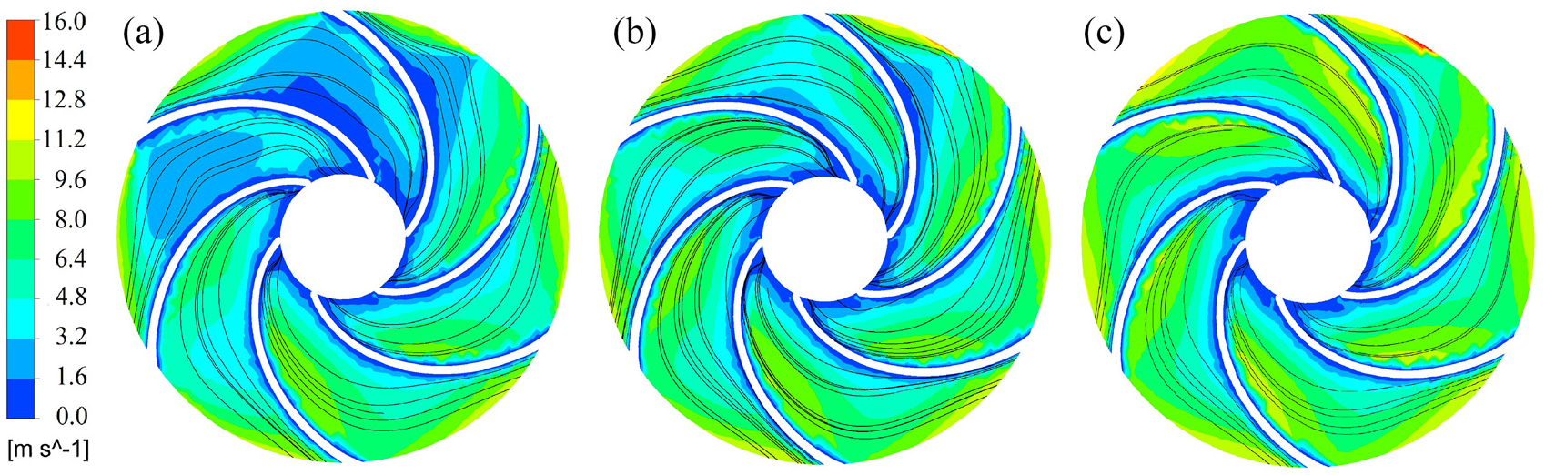
The relative flow velocity distributions in the impeller for the original and optimized variants at 0.8Q_d, 1.0Q_d, and 1.2Q_d are shown in Figures 10 and 11. Both Figures show the velocity at the center of the channel cross-section.

Figure 10.

Relative velocity distributions of original impeller: (a) 0.8Q_d, (b) 1.0Q_d, and (c) 1.2Q_d.

Figure 11.

Relative velocity distributions of the optimized impeller: (a) 0.8Q_d, (b) 1.0Q_d, and (c) 1.2Q_d.

For the original impeller, at flow rates of 0.8Q_d and 1.0Q_d, there are large regions with low relative velocity in each impeller channel (Figure 10), while some channels contain one or more vortices. As the flow rate increases, the vortices become less pronounced or even disappear in the original scheme.

In the optimized variant, some channels are less than optimally filled, resulting in regions of low relative velocity, at flow rate of 0.8Q_d, while vortices are absent (Figure 11). As the flow rate increases, the region with low relative velocity decreases, and the filling of each channels is relatively uniform. This explains the higher efficiency characteristics curve of the modified runner (Figure 6 compared to Figure 8).

We note, that in the original impeller, the velocity on the suction side is prone to be smaller than it on the pressure side, which is caused by the unreasonable design of the original scheme. The excessive blade outlet angle and small wrap angle lead to the wake area near the suction side of the impeller exit. While in the optimized variant, due to the action of inertia, reverse vortices, namely axial vortices, are generated in the impeller passage. The relative velocity in the impeller is the combination of the above-mentioned vortices and the through-flow, so the relative velocity on the pressure side is smaller than the suction side.

The absolute velocity distributions in the impeller and volute for both schemes under three flow rates of 0.8Q_d, 1.0Q_d, and 1.2Q_d are shown in Figures 12 and 13.

Figure 12.

Absolute velocity distributions of the original impeller and the volute: (a) 0.8Q_d, (b) 1.0Q_d, and (c) 1.2Q_d.

Figure 13.

Absolute velocity distributions of the optimized impeller and the volute: (a) 0.8Q_d, (b) 1.0Q_d, and (c) 1.2Q_d.

It can be seen from Figures 11 and 12 that the absolute velocity of the fluid increases gradually from the inlet to the outlet of the impeller under the influence of the centrifugal force. The absolute velocity at the pressure surface of the blade is smaller than that at the suction surface of the blade, as explained above in relation realization of the blade angles. As the fluid flows into the spiral, the absolute velocity gradually decreases due to the diffusion structure of the volute. Comparing both schemes, the absolute velocity in the impeller channel of the optimized variant is lower than that of the original scheme. Thus, the hydraulic loss in the impeller channel of the optimized variant is lower than that of the original scheme.

Overall, both the relative velocity distribution and the absolute velocity distribution in the impeller of the optimized variant are better than in the impeller of the original scheme.

Pressure distribution

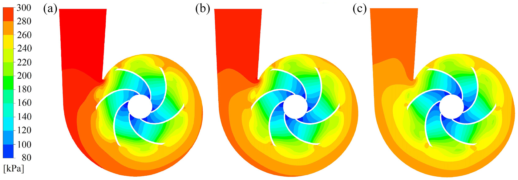
Figures 14 and 15 show the pressure distribution in the impeller and the volute of two schemes under the flow rates of 0.8Q_d, 1.0Q_d, and 1.2Q_d.

Figure 14.

Pressure distributions in the original impeller and volute: (a) 0.8Q_d, (b) 1.0Q_d, and (c) 1.2Q_d.

Figure 15.

Pressure distributions in the optimized impeller and volute: (a) 0.8Q_d, (b) 1.0Q_d, and (c) 1.2Q_d.

From Figures 14 and 15, it can be seen that pressure increases gradually from the impeller inlet to the impeller outlet due to the centrifugal force. The pressure on the pressure side of the blade is higher than the pressure at the suction side. Therefore, the suction surface of the impeller inlet is a place where cavitation is most likely to occur. As the fluid flows into the volute, the static pressure gradually increases due to the diffusion structure of the volute. As the flow increases, the static pressure in the impeller and volute gradually decreases, and the decrease in the static pressure in the volute outlet is more pronounced. Comparing the two schemes, the area of low pressure in the impeller inlet of the original scheme is larger than that in the impeller inlet of the optimized variant. Cavitation occurs more easily when the pump is used with the impeller of the original scheme. All the above points show that the pressure distribution in the impeller and volute of the optimized variant is better compared to the original scheme.

Pressure fluctuations

To analyze the pressure pulsations in the volute, the unsteady numerical simulation of the internal flow in pumps with different impellers was performed. For quantification, the pressure fluctuation coefficient is introduced as follows:

C_{p} = \frac{Δ p}{0.5 ρ u_{2}^{2}}

(1)

where Δp is the difference between the instantaneous pressure and the mean pressure, ρ is the fluid density, and u₂ is the circumferential velocity of the impeller outlet.

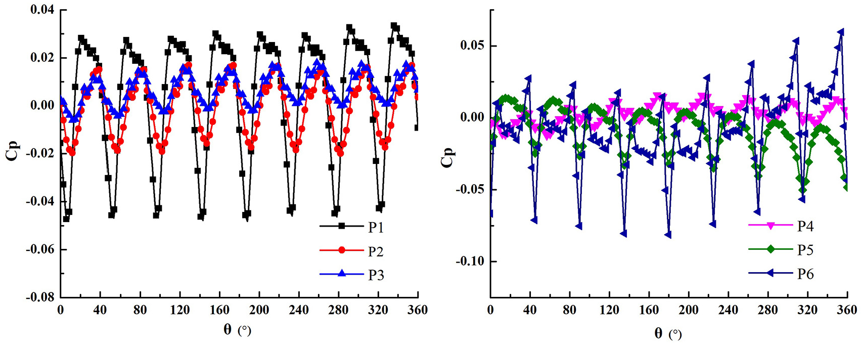
Time-domain plots of the pressure fluctuations in monitoring points are shown in Figures 16 and 17. The results are shown for one revolution of the impeller and for rate 1.0Q_d. The horizontal coordinate θ represents the angle at which the impeller rotates for one cycle, and the longitudinal coordinate C_p is the pressure fluctuation coefficient of the monitoring points computational according to equation (1).

Figure 16.

Time domain diagrams of pressure fluctuation at monitoring points of original scheme.

Figure 17.

Time-domain diagrams of pressure fluctuations at monitoring points of the optimized variant.

From Figures 16 and 17, it can be seen that during the rotation of the impeller, eight maxima and eight minima of the pressure fluctuations occur periodically for the original impeller (six maxima and six minima for the optimized impeller), both corresponding to the blade passes. The reason for this phenomenon is that as the impeller rotates, each monitoring point is alternately in the high and low-pressure regions of passing blades. The pressure fluctuations at monitoring point P6, the volute tongue, are higher than those at the other monitoring points, where the interaction between the impeller and the volute is relatively strong.

Comparing the two schemes, the pressure fluctuations in the volute with the impeller of the original scheme are lower than in the volute with the impeller of the optimized variant, especially in the volute tongue. In the hydraulic design of impeller and volute, the placement angle of the volute tongue should be equal to the absolute flow angle of the impeller outlet, so as to reduce the impact of liquid flow. In this paper, the blade number of impeller was adjusted, and the absolute flow angle at the impeller outlet was changed as a result. However, the parameter of the volute was not adjusted accordingly. Hence, the phenomenon above appeared.

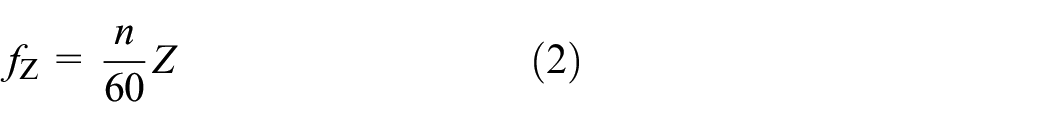
The pressure fluctuation in the frequency domain was obtained by fast Fourier transform of the data in the time domain. In order to analyze the characteristics of the frequency domain more clearly, the frequency value is dimensionless through the blade passing frequency f_n. The blade passing frequency f_z is introduced as follows:

f_{Z} = \frac{n}{60} Z

(2)

Figures 18 and 19 show the frequency domain plot of pressure fluctuation at the monitoring points. Figure 18 shows that the main frequency of pressure fluctuation at the monitoring points P1, P2 in the original scheme is at 800 Hz, which corresponds to BPF of the impeller and the main frequency of pressure fluctuation at the monitoring points P3, P4, P5, and P6 in the original scheme is at 100 Hz, which corresponds to APF of the impeller. It can also be found that the pressure pulsation of the monitoring point in the original scheme has an obvious wide band in the low-frequency region, which is related to the unstable flow in the impeller of the original scheme. Figure 19 shows that the main frequency of pressure fluctuation at each point in optimized variant is at 600 Hz, which corresponds to BPF of the impeller. The amplitude of pressure fluctuation at the main frequency at BPF gradually decreases spatially with the flow downstream along the spiral. Thus, the pressure fluctuations gradually decrease with the expansion of the volute passage. In the high-frequency range the pressure fluctuations at the monitoring points P1, P2, P3, P4, and P5 are small, while the pressure fluctuations at the monitoring point P6 are again much stronger. The amplitude of pressure fluctuation at the monitoring point P5 is higher than at points P2, P3, and P4, which is due to the complex flow conditions at the volute tongue, although it is located some distance downstream from the impeller exit or tongue. Comparing the two schemes, the overall pressure fluctuations in the whole volute with the optimized impeller are similar to those of the original impeller.

Figure 18.

Frequency domain diagrams of pressure fluctuations at monitoring points of the original scheme.

Figure 19.

Frequency domain diagrams of pressure fluctuations at monitoring points of the optimized variant.

Conclusions

In this work, steady state and transient CFD analysis of several centrifugal pump impellers were performed by commercial software CFX. The main conclusions can be summarized as follows:

The efficiency of the pump can be improved by increasing the wrap angle and the blade outlet angle appropriately while reducing the number of blades. At the design flow rate, the efficiency of the original scheme is 55.5%, and the efficiency of the optimized variant increases by 4.8%–60.3%. The head of the two schemes meets the design requirements although the head of the optimized variant is lower than that of the original scheme.

Instead of adopting the multi-factor and multi-level optimization method, with the help of numerical simulation results and theoretical analysis to optimize the automotive coolant pump, not only can complete the optimization better but also can reduce the workload greatly.

At low flow rates and designed flow rates, one or more vortices appear in selected channels of the original scheme or even block individual channels, while no vortices are present in the channels of the optimized variant. The unstable flow with vortex will affect the main frequency of pressure pulsation and the low frequency of pressure pulsation amplitude in the volute.

Although the efficiency of the automotive coolant pump can be improved by adjusting the impeller parameters On the basis of satisfying the head, it may cause the mismatch of volute and make the unstable flow characteristics of the pump worse.

Footnotes

Handling Editor: Chenhui Liang

Declaration of conflicting interests

The author(s) declared no potential conflicts of interest with respect to the research, authorship, and/or publication of this article.

Funding

The author(s) disclosed receipt of the following financial support for the research, authorship, and/or publication of this article: The paper was supported by the National Natural Science Foundation of China (51779106, 51979126), the Priority Academic Program Development of Jiangsu Higher Education Institutions (PAPD), and Slovenian Research Agency under research program Energy Engineering P2-0401.

ORCID iD

Linglin Jiang

References

Wagner

Paradis

Marotta

, et al. Enhanced automotive engine cooling systems: a mechatronics approach. Int J Veh Des 2002; 28(1–3): 214–240.

Wang

Liang

Hao

, et al. Comparison of electrical and mechanical water pump performance in internal combustion engine. Int J Veh Syst Model Test 2015; 10(3): 205–223.

Cho

Jung

Filipi

, et al. Application of controllable electric coolant pump for fuel economy and cooling performance improvement. J Eng Gas Turbines Power 2007; 129(1): 43–50.

Negandhi

Jung

Shutty

Active thermal management with a dual mode coolant pump. SAE Int J Passenger Cars Mech Syst 2013; 6(2): 817–825.

Setlur

Wagner

Dawson

, et al. An advanced engine thermal management system: nonlinear control and test. IEEE/ASME Trans Mechatron 2005; 10(2): 210–220.

Tan

Liu

, et al. Effect of blade wrap angle on performance of a single-channel pump. Exp Tech 2018; 42(5): 481–490.

Huang

Zhang

, et al. Energy performance prediction of the centrifugal pumps by using a hybrid neural network. Energy 2020; 213: 1–15.

Pei

Yuan

, et al. Effects of blade thickness on hydraulic performance and structural dynamic characteristics of high-power coolant pump at overload condition. Proc IMechE, Part A: J Power Energy 2018; 232(8): 992–1003.

Zhang

Guo

Yang

, et al. Blade shape optimization of centrifugal pump impeller with adjoint method. J Drain Irrig Mach Eng 2014; 32(11): 943–954 (in Chinese).

10.

Wang

Luo

, et al. Multi-condition optimization and experimental verification of impeller for a marine centrifugal pump. Int J Nav Archit Ocean Eng 2019; 12: 71–84.

11.

Zhang

Liu

Gao

, et al. Effects of modifying the blade trailing edge profile on unsteady pressure pulsations and flow structures in a centrifugal pump. Int J Heat Fluid Flow 2019; 75: 227–238.

12.

Tang

Jia

Ding

, et al. Experimental investigation on thermal management performance of an integrated heat sink with a piezoelectric micropump. Appl Thermal Eng 2019; 161: 114053.

13.

Tao

Wagner

JR.

An engine thermal management system design for military ground vehicle: simultaneous fan, pump and valve control. SAE Int J Passenger Cars Electron Electr Syst 2016; 9(1): 243–254.

14.

Feng

TY.

Calibration and match on electronic water pump to vehicle internal combustion engine. Shenyang: Shenyang Ligong University, 2018 (in Chinese).

15.

The study of characteristics prediction of car pumps based on hydraulic loss model. Shanghai: Shanghai Jiao Tong University, 2012 (in Chinese).

16.

Liu

Numerical simulation and performance prediction of car pumps. Shanghai: Shanghai Jiao Tong University, 2013 (in Chinese).

17.

Bai

Simulation analysis of flow field in centrifugal cooling water pump of engine. Changchun: Jilin University, 2018 (in Chinese).

18.

WQ.

The research of cavitation mechanism in engine cooling water pump under thermo-dynamic effect. Jiangsu: Jiangsu University, 2016 (in Chinese).

19.

Wickerath

Fournier

Durand

, et al. Fully variable mechanical coolant pump for commercial vehicles. MTZ worldwide 2011; 72(1): 28–33.

Optimization and CFD performance analysis of an automotive coolant pump

Abstract

Keywords

Introduction

Computation model and research method

Computation model

Mesh and independence check

Numerical computation method

Boundary conditions

Arrangement of monitoring points

Experiment

Results and analysis of CFD modeling

Performance analysis

Velocity distribution

Pressure distribution

Pressure fluctuations

Conclusions

Footnotes

Declaration of conflicting interests

Funding

ORCID iD

References