Sage Journals: Discover world-class research

Abstract

This work deals with a model development to predict the availability of continuous systems at the open pits using the artificial neural networks. The main idea of this work is to improve the analytical approach with initial assumption that the time length distributions of a faulty system have an exponential distribution. Data related to the I ECC(excavator, conveyors, crushing plant) system of the Open Pit Drmno Kostolac are used for this work. The aim of this work is to improve a model for predicting the availability of continuous systems at the open pits. On the basis of $RMSE$ , $MAE$ , and $R^{2}$ values, presented in this work, it is concluded that the model, obtained by the use of neural network, has a higher predictive power compared to the analytical approach. A corresponding simulation is created on the basis of obtained model that should a scope of the system availability for each type of failure. Also, a more precise image of the availability of continuous systems at the open pits is given on the basis of simulation.

Keywords

Systems ECC system open pit mining failure availability analytical approach artificial neural networks simulation

Introduction

The aim of this work is to improve a model for predicting the availability of continuous systems at the open pits. Based on a new model, an image of the system state is defined having a role in planning and control of exploitation, adoption an appropriate maintenance strategy, all with the aim of stable production and cost reduction.

Coal is the basic energy fuel in electricity production. Continuous systems are used at the open pits of the Electric Power Industry of Serbia for coal mining. These are the high-capacity complex excavation systems whose operation is crucial for a reliable supply of coal to the Thermal Power Plant. Related to this, the availability of one system was analyzed on the example of the Open Pit Drmno. Coal exploitation in the Kostolac Basin began in 1870. The Open Pit Drmno is the only active mine in the Kostolac Basin with production of 25% of coal (lignite) in Serbia, see Bugarić et al.¹

In the previous period, the growth of coal capacity was designed from the current 9 × 10⁶ to 12 × 10⁶ t/year and overburden from 40 × 10⁶ to the maximum 55 × 10⁶ m³/year at the Open Pit Drmno. Coal excavation is carried out by two ECC systems with one export conveyor, with occasional engagement of dragline excavator as necessary equipment. The excavated coal from both systems is transported by a collective conveyor to a distribution bin and further to the Crushing Plant, stockpile, and Thermal Power Plant. The ECC systems are systems that consist of the following elements: bucket wheel excavator, series of conveyors, and crushing plant. If there is a failure of one element of the ECC system, the whole system stops working, see Bugarić et al.¹

Literature review

In recent years, the published works on the use of machine learning in the field of mining have indicated that the artificial neural networks, as a method of machine learning, have an increasing application in the field of mining. Most of the works are related to the blasting process, see references.^2–38 In addition to the works, related to the mining process, there are also works in which models are developed for detecting the geomechanical anomalies,^39–41 analysis of available resources,^42–45 assessment the impact of mining works on the environment.^46,47 The machine learning method is also used for risk assessment of landslides at the open pit,⁴⁸ visual detection of objects at the open pit that can classify workers and mining machinery,⁴⁹ or prediction the health risks of drivers caused by vibrations during truck transport.⁵⁰

ECC system

The most general definition of a system describes it as a functional unit of several interconnected elements. Within the coal mining system, continuous systems represent the systems with the greatest complexity. The basic function of continuous systems is excavation, transport, and disposal of coal, which can be simply described as the coal production. These systems with continuous operation provide a continuous, uninterrupted flow of material from the place of excavation to the place of disposal, which conditions a high functional connection of its elements. The main objective of continuous systems in coal production is the realization of stable and reliable production of suitable capacity. These systems are connected in a series connection as it can be seen in Figure 1.

Figure 1.

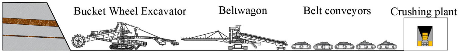
Overview of the ECC system.

I ECC system

This work presents a Case Study for determining the availability of a continuous system on coal from the Open Pit Drmno, which consists of the following elements (subsystems): SRs 400 bucket wheel excavator, BRs 2400 beltwagon, a series of belt conveyors, and Crushing Plant. The layout of the ECC system is shown in Figure 2.

Figure 2.

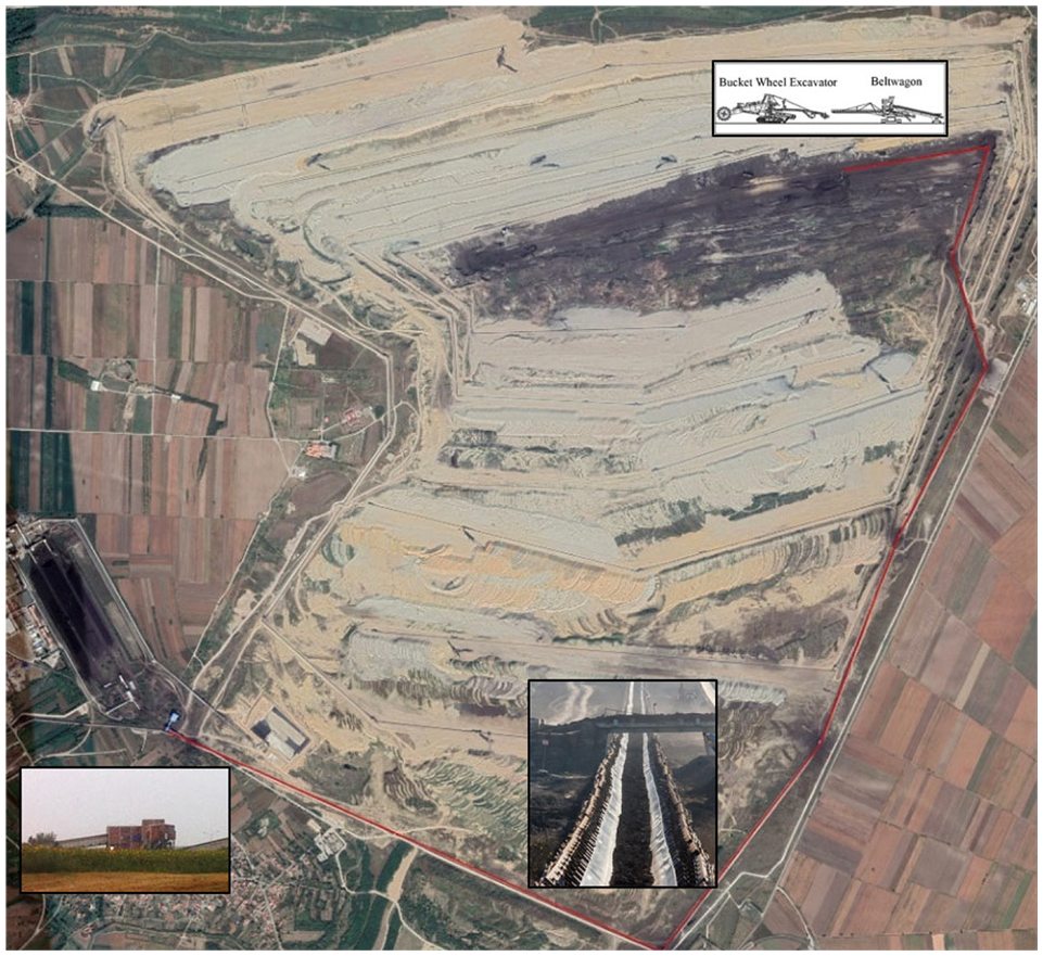
Layout of the ECC system at the Open Pit Drmno.

Subsystem characteristics

SRs400 bucket wheel excavator

Bucket-wheel excavator represents a self-propelled continuous action machine intended for excavation of overburden and ore at the open pits. Material excavation is done with buckets that are evenly distributed and attached to the rotor rim. Simultaneously with the rotation of rotor in a vertical plane and rotor boom rotation together with the platform in a horizontal plane, each bucket digs out a section from massive, which is determined by the shape and geometric parameters. By the rotor rotation and coming out of full buckets in the unloading sector zone, the material is emptied from buckets, handed over to the receiving belt conveyor on the rotor boom and further in order, depending on the number of conveyors on the excavator, the last unloading conveyor.^51–58

Bucket-wheel excavator are considered to be one of the most complex machines and are characterized by continuous development and modernization during their lifetime.⁵⁹

The SRs 400.14/1.5 bucket-wheel excavator operates within the I ECC system. The manufacturer of this bucket-wheel excavator is manufactured by the German company Takraf. The bucket-wheel excavator was purchased in 1985.⁶⁰

The bucket-wheel excavator is in itself a very complex machine system. Like any system, it is composed of a number of subsystems:

− Subsystem for excavation,

− Subsystem for excavator movement,

− Subsystem of receiving conveyor,

− Subsystem of conveyor stacker,

− Subsystem for swiveling the upper structure.^1,61

According to the German classification, the bucket-wheel excavators are divided into the following classes: A (compact excavator), B (excavator with C frame), and C (giant excavator) according to the basic construction characteristics (Figure 3).^{51,52,57,58,62}

Figure 3.

Types of bucket-wheel excavators.⁵¹

This excavator belongs to the group of compact rotary excavators. Compact excavators have a relatively short boom in relation to the diameter of working wheel.^1,62

The rotary excavator operates in very difficult conditions, where high productivity, reliability, availability, and safety at work are constantly expected from it as a carrier of production. The operation effects of mining machines depend on the reliability, their functioning, technical and technological performances, handling, maintenance, logistic support, adaptability – compliance of the relationship between the performances of machines and characteristics of the working environment.^1,63

Figure 4 shows the SRs 400.14/1 bucket-wheel excavator. Table 1 presents the structural and technical characteristics of the SRs 400.14/1 bucket-wheel excavator.

Figure 4.

SRs 400.14/1 bucket-wheel excavator, see Kričković.⁶⁰

Table 1.

Structural and technical characteristics of the SRs 400.14/1 bucket-wheel excavator, see Milovanović et al.⁶⁴

SRs 400.14/1 bucket wheel excavator
Theoretical capacity (m³/h)	2800
Wheel diameter (m)	7.5
RT installed wheel drive power (kW)	900
Specific excavation force (N/cm)	910
Nominal bucket volume (m³)	0.55
Number of buckets	12
Number of bucket unloading (1/min)	70–84
Excavation height (m)	14
Excavation depth (m)	1
Boom length (m)	14.5
Unloading belt length (m)	22.5
Excavator length (m)	42
Excavator width (m)	12
Excavator height (m)	13
Excavator mass in operation (t)	530

BRs 2400 beltwagon

Beltwagon represents connection between the excavation and transport equipment within the continuous system. Its mobility enables an increase of technological parameters of the excavator operation according to the plan and height, more efficient use of the bucket-wheel excavator within the bench system of the open pit and better time utilization. According to the construction, they can be: rigid or with rotating booms. The capacity should be aligned with the excavation equipment capacity.

Figure 5 presents the BRs 2400 beltwagon. Table 2 gives structural and technical characteristics of the BRs 2400 beltwagon.

Figure 5.

BRs 2400 beltwagon, see Kričković.⁶⁰

Table 2.

Design and technical characteristics of the BRs 2400 beltwagon, see Milovanović et al.⁶⁴

Beltwagon BRs 2400
Theoretical capacity (m³/h)	3800
Guaranteed capacity (m³/h)	2400
Height (m)	17
Width (m)	13
Length (m)	58.3
Mass (t)	286
Unloading height (m)	13
Conveyor speed (m/min)	6
Belt width (m)	1.4
Unloading boom length (m)	35.7

Belt conveyors

Continuous transport with conveyors is increasingly used at the open pits of medium and large capacities.⁶⁵

Transport of overburden and coal is one of the most important parts of the technological process of lignite exploitation. Transport costs account for 40%–60% of the total operating costs.⁶⁶ Figure 6 shows the basic parts of the conveyor.

Figure 6.

Basic parts of a belt conveyor https://instrumentationtools.com/conveyor/.⁶⁷

The basic parts of a belt conveyor are:

− endless rubber belt that represents the carrying and haulage body,

− supporting structure (belt) of a conveyor that carries the upper and lower sets of pulleys,

− drive station,

− return or end station,

− tightening device,

− cleaning device for belts and drums,

− loading or unloading part,

− apparatus for control and automatic control.⁵²

Table 3 gives the design and technical characteristics of a belt conveyor on the I ECC system.

Table 3.

Design and technical characteristics of a belt conveyor on the I ECC system, see Milovanović et al.⁶⁴

I ECC system	Belt conveyors B = 1800 mm	Belt conveyors B = 2000 mm
Theoretical capacity (m³/h)	7200	6600
Belt width (mm)	1800	2000
Belt speed (m/s)	5.2	4.65
Installed power of the main drive (kW)	4 × 630	4 × 1000
Type of rubber belt	St 3150	St 2500 16/8
Belt bed angle (°)	45	36
Type of belt tension	Winch	1400
Installed winch power (kW)	2 × 22	26
Type of transport movement	Pair of crawlers	Pair of crawlers
Station speed (m/min)	5.8	4
Installed power (kW)	4 × 30	3 × 25

Belt conveyors I ECC:

− Bench conveyor – U-I-1,

− Bench conveyor – U-I-3,

− Bench conveyor – U-I-2,

− Connecting conveyor – UZ-1,

− Connecting conveyor – UZ-2,

− Connecting conveyor – UZ-2.1,

− Connecting conveyor – UZ -3,

− Connecting conveyor – UZ -4. see Milovanović et al.⁶⁴

Crushing plant

Figure 7 shows the Crushing Plant at the Open Pit Drmno Kostolac.

Figure 7.

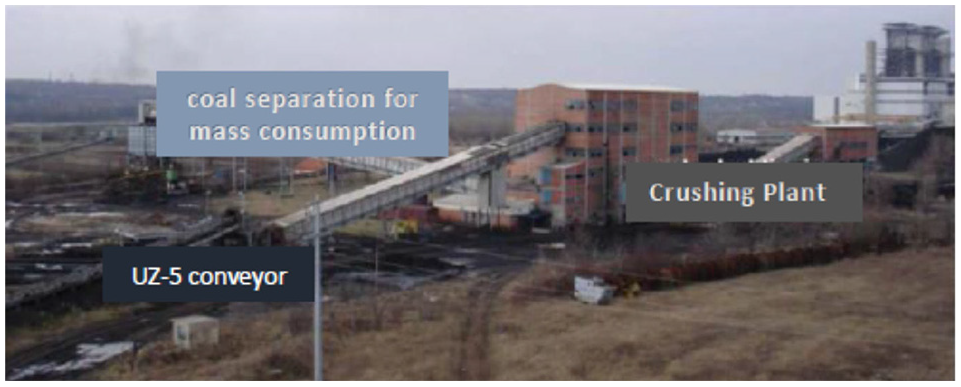
Crushing Plant, see Milovanović et al.⁶⁴

Materials and methods

Description of the data set

There is no machine (continuous system) that operates without failure. Failures on continuous systems have negative production and economic effects. A failure or breakdown is a cessation of element ability to perform its function. There is a complete (machine shutdown) and partial failure (machine works but with deteriorated characteristics), see Ivković.⁶⁸

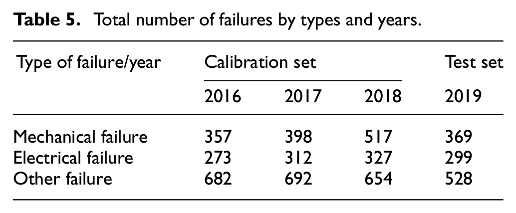
On the basis of data, obtained from the Electric Power Industry of Serbia, which also includes the Open Pit Drmno, a time-related database was formed for mechanical (damage of the upper structure bearings, cracking of crawlers, tooth replacement, etc.), electrical (cable breakdown, interruption of TT connection, blockade breaking, etc.), and other failures (overhaul, service, conditional standstill due to the bad weather conditions, etc.) of the I ECC system (SRs 400) for a period of 4 years (2016, 2017, 2018, and 2019), see Bugarić et al.¹

Program language in the Python 3.7.7 in the PyCharm editor was used for data processing, as well as for further analysis and availability prediction of continuous systems.

Table 4 shows a part of database. The database contains data related to the date, facility on which the failure (delay) occurred, exact time and date of delay beginning and end, as well as the total time in delay.

Table 4.

Database form.

Date	Months	Year	System	Object	Failure	Start of failure	End of failure	Downtime	Total downtime in minutes	Notes	Shift
1.1.2016	January	2016	ECC SRs-400	BWE SRs-400	Electrical	10:00:00	10:50:00	00:50	50	/	1
1.1.2016	January	2016	ECC SRs-400	Crushing plant	Other	13:00:00	14:30:00	01:30	90	/	1
1.1.2016	January	2016	ECC SRs-400	BWE SRs-400	Electrical	19:00:00	19:10:00	00:10	10	/	2

The basic idea is that the application of neural networks can improve the analytical approach of determining the availability of continuous systems at the open pits, which uses the assumption that failure rates have an exponential distribution. In order to properly demonstrate the advantage of neural networks, it is necessary that both the calibration set (in the case of neural network, the calibration set is further divided into training and validation set) and the test data set for both models are matched. The same test statistics RMSE (Root Mean Square Error) and MAE (Mean Absolute Error) will be used in both cases. These statistics are defined by:

RMSE = \sqrt{MSE}, MSE = \frac{1}{n} \sum_{i = 1}^{n} (y_{i}^{a} - y_{i}^{p})^{2}

(1)

MAE = \frac{1}{n} \sum_{i = 1}^{n} | y_{i}^{a} - y_{i}^{p} |,

(2)

where $y_{1}^{a}$ , $y_{2}^{a}$ ,…, $y_{n}^{a}$ are the actual values, and $y_{1}^{p}, y_{2}^{p}$ , …, $y_{n}^{p}$ are the values predicted by the model.

As the additional statistics, the determination coefficient $R^{2}$ is used, that is defined by:

R^{2} = 1 - \frac{\sum_{i = 1}^{n} {(y_{i}^{a} - y_{i}^{p})}^{2}}{\sum_{i = 1}^{n} {(y_{i}^{a} - \frac{1}{n} \sum_{i = 1}^{n} y_{i}^{a})}^{2}} .

(3)

The initial database is divided into three groups based on the type of failure (mechanical, electrical, and other failures), and then each part is divided into a calibration set and test data set. The calibration data set contains data for the appropriate type of failure on which the model is developed, and covers a period of 3 years (2016, 2017, and 2018). The test data set contains data on which the power of obtained models for the appropriate types of failure is assessed, and includes the last year of data in the database (2019). In the case of machine failures, the percentage of data, on which the model is trained, is 77.51%. In the case of electrical failures, it is 75.24%, while the percentage for other failures is 79.34%.

Table 5 presents the total number of failures by type and years.

Table 5.

Total number of failures by types and years.

Type of failure/year	Calibration set			Test set
	2016	2017	2018	2019
Mechanical failure	357	398	517	369
Electrical failure	273	312	327	299
Other failure	682	692	654	528

The following Table 6 presents the mean value, standard deviation, minimum value, first quantile value, median, third quantile value, and maximum value before and after outlayer treatment on the calibration data set for each type of failure. The method used in the treatment of outliers is the Z-Score method.

Table 6.

Overview of the most important descriptive statistics on the calibration data set before and after outlayer treatment.

	Count	Mean	Std	Min	First quartile	Median	Third quartile	Max
Mechanical failure
Before	1297	76.8966	726.9258	5.0000	10.0000	20.0000	40.0000	24,480.0000
After	1289	40.4111	65.8817	5.0000	10.0000	20.0000	40.0000	950.0000
Electrical failure
Before	950	58.0421	95.4353	5.0000	15.0000	30.0000	55.0000	820.0000
After	920	43.7282	44.4606	5.0000	15.0000	30.0000	55.0000	290.0000
Other failure
Before	2033	175.0344	2125.5011	5.0000	35.0000	70.0000	115.0000	64,800.0000
After	2030	96.3522	108.60515	5.0000	35.0000	70.0000	115.0000	1840.0000

Extracting a large number of feature data and determining the distribution of failure intensity do not give a clear image of the statistical set, because a large number of classes is obtained, so dividing the statistical data set into equal intervals is carried out. The total interval of the statistical set $I = t_{\max} - t_{\min}$ , where $t_{\min}$ and $t_{\max}$ are the minimum and maximum failure lengths, is divided into $5 lo g_{10} (n)$ equal parts, where n is the total data number for a particular type of failure, see Djurić.⁶⁹ In case of machine failures, there are 16 intervals of 59.0625 min, 15 intervals of electrical failures of 19.0000 min, and 17 intervals of other failures of 107.9411 min.

Figure 8 presents the distribution of failures for each type of failure by year.

Figure 8.

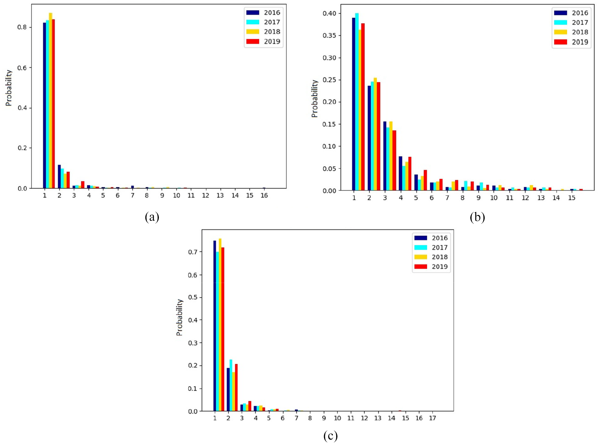
Distribution of failures for each type of failure: (a) mechanical failure by years, (b) electrical failure by years, and (c) other failure by year.

Methodology

Availability is calculated on the basis of a time state picture, in which the times when the system is in good condition, the “up-time,” change with the times when the system is out of order, the “down-time.” The time state picture can be shown in Figure 9. 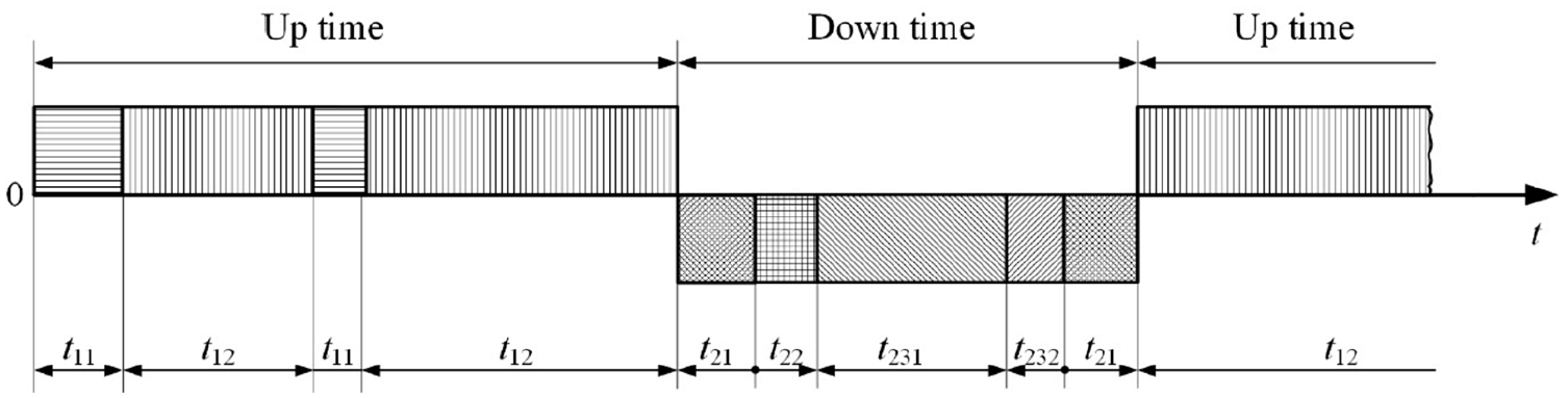The time when the system is in good condition can be divided into inactive time, that is the time while the system is waiting for work (stand-by) ( $t_{11}$ ) and the time when the system is working ( $t_{12}$ ). Time, when the system is in failure, is divided into: organizational time ( $t_{21}$ ), logistic time ( $t_{22}$ ), and active repair time ( $t_{23}$ ) which can be the time for corrective repairs ( $t_{231}$ ) and time for preventive repairs ( $t_{232}$ ), see Djenadic et al.⁷⁰

Figure 9.

Time picture of the state, see Djenadic et al.⁷⁰

Availability is defined as the quotient of the total time during which the system is in good condition and the total time that makes up the time in good condition and time in failure (operational availability), see Djenadic et al.⁷⁰

A (t) = \frac{\sum t_{11}, t_{12}}{\sum t_{11}, t_{12}, t_{21}, t_{22} t_{231}, t_{232}}

(4)

One of the most common approaches in determining the availability of continuous systems is based on the assumption that the lengths of time the machine has failed to have an exponential distribution (see Djenadic et al.⁷⁰). Although the values of $RMSE$ , $MAE$ i $R^{2}$ statistics for the stated analytical approach on the available data are large, see Table 6, the assessment of distribution the lengths of time the machine has failed, is performed by a model obtained using the neural networks. The obtained model better describes the actual state of data. By applying the obtained neural network, the failure lengths are further generated, on the basis of which the availability of a continuous system in a period of 1 year is calculated. Figure 10 schematically presents the flowchart of methodology.

Figure 10.

Flow chart methodology.

The research process of this study is as follows:

Step 1 – Loading and processing of raw data

Using the appropriate Python libraries (pandas, numpy) to load and organize the data, all the necessary processes were performed to prepare the data for further analysis and create an appropriate model for predicting system availability.

Step 2 – Preparation of data for the model

The input variables which effect on the availability of continuous mining system, in this study, are interval limits and year. They are ranked according to the experiment sequence, and they are splitted into the calibration and test values.

Step 3 – Deep learning of data failure intensities

The number of the input layers, hidden layers, and output layers are defined in the neural network framework. Also, in this step are chosen activation functions and optimizer.

Step 4 – Choice of model architecture and hyperparameters

The batch size and learning rate are set to neural network framework. The training process goes on repeatedly until the neural network convergence.

Step 5 – Model evaluation on a test set

When neural network model has been trained, the output arguments are obtained as the predictions. The $RMSE$ , $MAE$ , and $R^{2}$ values are used to compare the predicted and the actual values.

Step 6 – Simulation

In this step are defined simulation which described the availability of continuous mining system in the next year.

Results and discussions

Analytical approach and exponential distribution

The analytical approach (AP) of determining the availability of continuous systems at the open pits uses an assumption that the failure intensities take an exponential distribution EXP (λ) with a parameter λ, is also called a failure intensity. The density function pdf(x) and distribution function cdf(x) are determined by:

pdf (x) = {\begin{matrix} λ e^{- λ x}, & x \geq 0 \\ 0, & x < 0 \end{matrix}

(5)

and

cdf (x) = {\begin{matrix} 1 - e^{- λ x}, & x \geq 0 \\ 0, & x < 0 \end{matrix}

(6)

Using the property that the expectation of exponential distribution EXP (λ) is equal to 1/λ, the corresponding values of parameter λ for each type of failure are obtained. In the following Table 7, in addition to the values of the obtained parameter λ, the values $RMSE$ , $MAE$ , and $R^{2}$ are also stated, both on the calibration set and test data set for each type of failure.

Table 7.

Parameters of exponential distribution, the $RMSE$ , $MAE$ , and $R^{2}$ values.

	λ	$RMSE$	$MAE$	$R^{2}$
Mechanical failure
Test set	0.0130	0.0948	0.0400	0.7794
Calibration set		0.0998	0.0416	0.4016
Electrical failure
Test set	0.0172	0.0364	0.0195	0.8789
Calibration set		0.0448	0.0261	0.6270
Other failure
Test set	0.0057	0.0714	0.0306	0.8270
Calibration set		0.0765	0.0325	0.5592

Large deviations of the values predicted by the model and failure frequencies are observed in the shown graphics (Figure 11). Thus, the values of failure in the first interval are underestimated, and those in the second and third interval are overestimated.

Figure 11.

Theoretical curves and frequency of failures on (a) mechanical, (b) electrical, and (c) other failures.

Neural network approach

Neural network

Neural networks are the most popular method of machine learning, see Das and Behera.⁷¹ Artificial neural networks (ANNs) represent a branch of artificial intelligence, see Monjezi et al.³¹

The first artificial neural network is given by McCulloch and Pitts (1943) and since then has been popular and applicable in various fields of science and technology to solve the complex problems, see Sayadi et al.⁵

The artificial neural networks (computational) models are inspired by the structure and functioning of biological nervous systems. Trying to mimic the functioning of biological nervous systems makes them the adaptive systems that learn from examples, find dependencies between the data that do not seem to exist, find the new ways of data processing, or change their mode of operation to reach an optimum solution unlike the classical models that rely on linear programming, see Stojadinović.⁷²

The basic variant consists of fully connected neural networks that consist of the basic computational units, called neurons. The neurons are organized into layers so that the neurons of one layer receive as their input arguments the output arguments of all neurons of the previous layer, and forward their output arguments to all neurons of the next layer. All layers, whose neurons pass their output arguments to the other neurons, are called the hidden layers. The input arguments of the first layer are the input arguments of network, and the output arguments of the last layer are the output arguments of network. The output argument of each neuron is the value of activation function (in practice, ReLu, sigmoid, linear, exponential… are the most often used) over the linear combination of the input arguments of the observed neuron. Formally, the model is defined as follows:

h_{0} = x, h_{i} = g (W_{i} h_{i} + w_{io}), i = 1, 2, \dots, L,

(7)

where x is the input argument of network, L is the number of layers, $W_{i}$ is the matrix of non-free coefficients, and $w_{io}$ is the vector of free coefficients of the linear combination, while $g$ is the activation function, see Nikolić and Zečević.⁷³

Using the error function that compares the actual and predicted values, obtained from the neural network, the linear combination coefficient of input arguments for each neuron is changed. Changing the coefficients of linear combination of the input arguments for each neuron is done by the backpropagation algorithm that consists of three steps: calculating the output argument of network, calculating the error function that compares the actual and predicted values, and correcting the linear combination coefficients for each neuron.

In practice, the RMSE and MAE are the most commonly used for error functions.

LSTM networks

There are two basic problems of recurrent neural networks: the first concerns the problem of emerging and exploding gradients, while the second problem concerns the long-term storage of information and modeling the long-term dependencies in data. Both of these problems are overcome by the use of long short-term memory (LSTM), which is a complex network unit with a specific structure that allows control of reading and writing to the unit. The basic idea of LSTM is the existence of a so-called cell that keeps a hidden state, with control of writing, reading, and forgetting, which is done on the basis of learned rules. A specific formulation is given below ^73,74:

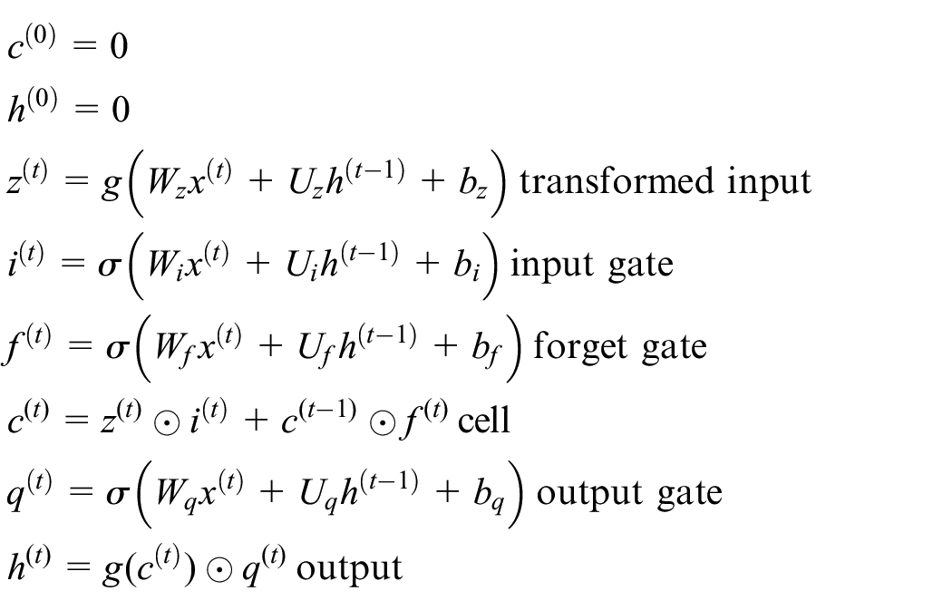
\begin{matrix} c^{(0)} = 0 \\ h^{(0)} = 0 \\ z^{(t)} = g (W_{z} x^{(t)} + U_{z} h^{(t - 1)} + b_{z}) transformed input \\ i^{(t)} = σ (W_{i} x^{(t)} + U_{i} h^{(t - 1)} + b_{i}) input gate \\ f^{(t)} = σ (W_{f} x^{(t)} + U_{f} h^{(t - 1)} + b_{f}) forget gate \\ c^{(t)} = z^{(t)} ⊙ i^{(t)} + c^{(t - 1)} ⊙ f^{(t)} cell \\ q^{(t)} = σ (W_{q} x^{(t)} + U_{q} h^{(t - 1)} + b_{q}) output gate \\ h^{(t)} = g (c^{(t)}) ⊙ q^{(t)} output \end{matrix}

where c denotes the cell that stores the LSTM unit state, z the transformed value of input, i the value of input gate, f the value of forget gate, q the value of output gate, and h the value of LSTM unit output. Each of the gates has its own set of parameters, marked with the appropriate index. The architecture of LSTM unit according to Goodfelow et al.⁷⁴ is given in Figure 12. Figure 13 shows the structure of the LSTM unit compared to the Standard Recurrent Unit (SRN).

Figure 12.

LSTM unit structure.^73,74

Figure 13.

LSTM unit structure (right) compared to the SRN unit (left).⁷³

The essence is quite simple. Each of the gates has the same structure as a unit of standard recurrent network and, based on the received input and associated parameters, it decides whether and to what extent it allows the execution of operation which is controlled, see Nikolić and Zečević.⁷³

For example, the input gate controls whether it will miss the input to cell, and it operates based on the input (first sum in the definition of input activation), and its state in the previous step (second sum) calculates the coefficient used to control the effect of input on the cell state. Similarly, the forget gate controls the effect of previous state of cell on the new state of cell in an analogous way. There are various modifications of the LSTM, but it is limited here to its form. The LSTM is important for two reasons. First, thanks to the gates that can control the input to the cell, the cell does not have to accept the input signals and, therefore can store information about distant parts of the sequence for a long time. Whether it should receive the input signals or not is something that is learned thanks to the fact that the input gate is parameterized. It should be kept in mind that in practice a large number of such units are used in parallel, so that while the others can process the current input, combine it with information from the former and similar.⁷³

Another reason of the LSTM significance is to mitigate the problem of emerging gradients. Namely, in the case of an ordinary recurrent network, the new value of hidden layer is obtained taking the output of that layer in the previous step as the input, transformed by the activation function. Addition of activation functions to the calculation threshold leads to multiplying the derivatives of activation functions in calculating the derivatives. By multiplying such numbers, the gradient disappears. On the other hand, when calculating a new cell value, there is no application of the activation function. Certainly, the previous value is multiplied by the forget gate value including the sigmoid activation function, so its derivative must appear somewhere in the gradient calculation, but the existence of paths in the computational graphics that are not affected by this problem, has a noticeable effect. For example, a standard recurrent network usually does not model well the dependence on a distance greater than a dozen steps. On the other hand, the recurrent networks with the LSTM unit successfully model the dependencies even at a distance of several hundred steps.⁷³

Neural network for determining the probability of failure in a certain time interval

The neural network, presented in this work, predicts the probability that the failure length is in a predetermined interval for a given year. Consequently, the input arguments of network are the interval and year limits, and the output argument is the probability that an arbitrary failure for a given year is within the interval limits.

Using a formula to determine a length of the optimal intervals into which the statistical set is divided,

\frac{t_{\max} - t_{\min}}{5 lo g_{10} (n)}

(8)

for each type of failure and year that is in the calibration data set, the interval limits and corresponding failure frequencies for a particular type of failure and year in which the failure occurred are defined. Additionally, the failure frequencies are determined for the interval limits, resulted from translation of the originally obtained intervals for k, 2k, 3k… minutes.

The optimal values for parameter k were obtained such as the value of RMSE statistics on a validation data set, which represents 20% of the randomly selected data from a part predicted for calibration, is minimized. In the case of all types of failures, the parameter k value is equal to 5. Furthermore, for each type of failure, the interval limits and corresponding failure frequencies in the test data set are defined in a similar way.

Furthermore, a neural network is defined for each type of failure. The neural network consists of two hidden layers (Figure 14). The type of neural network is Bidirectional long-short term memory (Bidirectional LSTM) implemented in the keras python library. The first hidden layer consists 128 neurons with ReLu activation function. The second hidden layer consists 256 neurons with sigmoid activation function. The activation function of output layer is the exponential function. The optimizer used in these modes is Adam optimizer with learning rate 0.0001. The MSE (defined in (1)) is an error function used in this work. Model development for each neural network was completed on 80% of data randomly selected from the calibration part (training set), while the remaining 20% was used for testing (validation set). The number of epochs for each model was 2000, while the value of batch size differed from the type of failures. For mechanical failures we used batch size 1000, the value of batch size for electrical failures was 300, while for other failures the value of mentioned parameter was 2000. The obtained models were tested on an independent data set (test set), which included the limits of the interval and the values of the corresponding probabilities for 2019. The input arguments of each neural network are the limits of interval and years, and the output argument of neural network is the probability of failure whose length is within a given interval for a given year. The activation functions used in this work are: ReLu, Sigmoid, and Exponential. Definitions and graphics of the mentioned functions are listed in Table 8. For example, the input arguments and output arguments, for electrical failure, are presented in the Table 9. The Figure 15 shows the values of error functions on each type of models. Table 10 presents the $RMSE$ , $MAE$ , and $R^{2}$ values on the calibration data set (training set and validation set) and test data set for each neural network.

Figure 14.

Neural Network architecture.

Table 8.

Definitions and graphics of the used functions.

Name	Function	Plot
ReLu	$g (x) = {\begin{matrix} x, & x \geq 0, \\ 0, & x < 0 . \end{matrix}$
Sigmoid	$g (x) = \frac{1}{1 + e^{- x}}$
Exponential	$g (x) = e^{x}$

Table 9.

The form of input and output arguments for electrical failure.

Input data			Output data
Interval limits		Year	Probability
5	24	2016	0.38869
5	24	2017	0.40000
5	24	2018	0.36257
10	29	2016	0.25795
10	29	2017	0.29846
10	29	2018	0.24269
15	34	2016	0.23322
15	34	2017	0.25538
15	34	2018	0.23684

Figure 15.

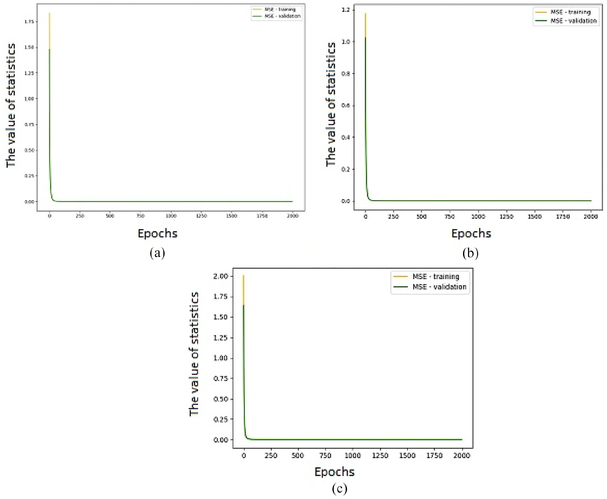
The values of error functions: (a) mechanical failure, (b) electrical failure, and (c) other failure.

Table 10.

$RMSE$ , $MAE$ , and $R^{2}$ (ANN) values.

	$RMSE$	$MAE$	$R^{2}$
Mechanical failure
Test set	0.0064	0.0038	0.9989
Validation set	0.0009	0.0009
Training set	0.0037	0.0021
Calibration set	0.0035	0.0019	0.9901
Electrical failure
Test set	0.0097	0.0064	0.9913
Validation set	0.0027	0.0023
Training set	0.0080	0.0047
Calibration set	0.0073	0.0042	0.9656
Other failure
Test set	0.0075	0.0040	0.9980
Validation set	0.0005	0.0005
Training set	0.0033	0.0014
Calibration set	0.0030	0.0012	0.9950

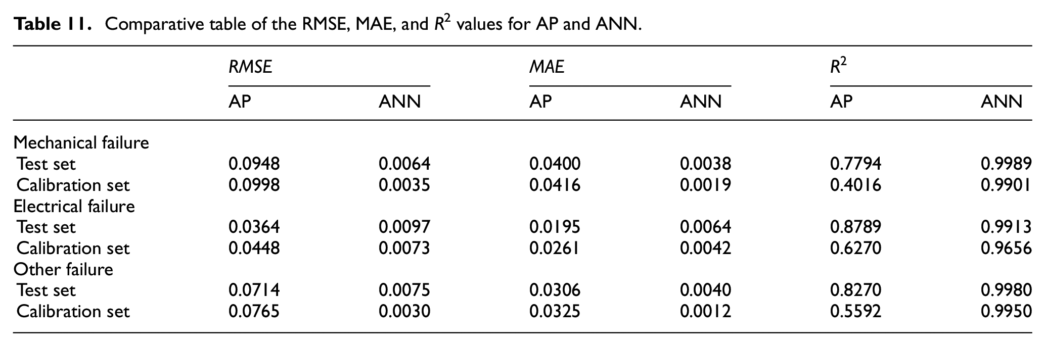
Comparative analysis of the analytical approach and model obtained using the neural network

Based on the $RMSE$ , $MAE$ , and $R^{2}$ values presented in Tables 7 and 10 and comparable Table 11, it is concluded that a model obtained using the neural network has a greater predictive power.

Table 11.

Comparative table of the RMSE, MAE, and R² values for AP and ANN.

	$RMSE$		$MAE$		$R^{2}$
	AP	ANN	AP	ANN	AP	ANN
Mechanical failure
Test set	0.0948	0.0064	0.0400	0.0038	0.7794	0.9989
Calibration set	0.0998	0.0035	0.0416	0.0019	0.4016	0.9901
Electrical failure
Test set	0.0364	0.0097	0.0195	0.0064	0.8789	0.9913
Calibration set	0.0448	0.0073	0.0261	0.0042	0.6270	0.9656
Other failure
Test set	0.0714	0.0075	0.0306	0.0040	0.8270	0.9980
Calibration set	0.0765	0.0030	0.0325	0.0012	0.5592	0.9950

Availability prediction

For the high-capacity mining systems such as the continuous coal excavation system (I ECC system), it is important to anticipate its availability to define the system condition picture necessary in the planning phase. Time when the system is not in operation entails the production and economic costs. This model has the role of assisting the responsible persons at the open pit in the planning and control of exploitation, adoption an appropriate maintenance strategy, all with the aim of stable coal production and cost reduction. The availability of a specific system as a whole is the basic input for production planning at the lignite open pits of Electric Power Industry of Serbia, but also other activities in the field of planning, monitoring production, or maintenance of equipment.

Figure 16 shows the failrue frequence curves determined by the neural network and by monitoring. On the basis of model, obtained from the neural network for initially defined intervals of the statistical data set, for each type of failure, the appropriate probabilities can be assigned with a failure length within the interval limits.

Figure 16.

Neural network and failure frequency curve: (a) Mechanical failure, (b) electrical failure, and (c) other failure.

Simulation

The $n_{test}$ of random numbers, where $n_{test}$ is the failure number in the test data set, is determined for each interval of initially divided statistical set for a certain type of failure (mechanical 369, electrical 299, and others 528).

If the random number is greater than the probability, obtained from the model that uses the neural network, it is considered that the failure did not occur. If the random number is less than the probability, it is considered that the failure occurred. In addition, it will be considered that a length of such generated failure is equal to the middle of observed interval. In this way, the total failure time of a continuous system with failure lengths in the observed interval should be obtained. The total failure time of continuous system on coal for a particular type of failure is obtained by addition the total failure time within each interval.

Observing all combinations of mechanical, electrical, and other failures, 1,000,000 different times that the system spent in failure are obtained. Based on the obtained results, 1,000,000 values for the system availability are obtained. Table 12 presents the basic statistics for simulated values of each type of failure, while Table 13 presents the basic statistics of simulated values for availability.

Table 12.

Overview of the most important statistics on simulation the total system time spent in failure.

	Count	Mean	Std	Min	First quartile	Median	Third quartile	Max
Mechanical failure	100	29,862.3181	2266.5836	24,677.4244	28,321.8228	29,833.8322	31,573.7639	34,565.8145
Electrical failure	100	16,723.0263	1257.2155	13,521.0652	15,911.0894	16,731.6305	17,610.8538	19,417.7923
Other failure	100	95,584.1608	6031.9218	80,970.9819	90,590.5612	95,398.9340	100,354.0578	107,943.9750

Table 13.

Overview of simulated values for simulation availability.

	Count	Mean	std	Min	First quartile	Median	Third quartile	Max
Simulation	1,000,000	0.7295	0.0124	0.6919	0.7198	0.7294	0.7389	0.7732

Conclusion

Based on the $RMSE$ , $MAE$ , and $R^{2}$ values, presented in Tables 7 and 10 and comparable Table 11, it is concluded that the model obtained using the neural network has a higher predictive power related to the probability that the fault length is in a certain time interval as shown in Figure 17. Based on the simulation, described in the previous chapter, the system availability can be expected to be in the range (0.7090, 0.7499) with a confidence level of 90%, in the range (0.70519, 0.7538) with a confidence level of 95%, and in the interval (0.6975, 0.7614) with a confidence level of 99%.

Figure 17.

Curve obtained by analytical procedure, neural network, and failure frequency: (a) mechanical failure, (b) electrical failure, and (c) other failure.

Footnotes

Acknowledgements

Gratitude to: Ministry of Education, Science and Technological Development of the Republic of Serbia. Mining and Metallurgy Institute Bor, Zeleni bulevar 35, Bor. Ministry of Mining and Energy, 11000 Belgrade, Serbia. PE Electric Power Industry of Serbia, Balkanska 13, 11000 Belgrade. PE Electric Power Industry of Serbia – Branch “TE-KO Kostolac,” Nikola Tesla 5-7, 12208 Kostolac.

Handling Editor: Chenhui Liang

Author contributions

Conceptualization, M.G. and S.S.; methodology, M.G.; validation, N.S. and A.M.; supervision, D.M.; writing-review and editing, M.G. and S.S.; visualization, M.G. and N.S.

Declaration of conflicting interests

The author(s) declared no potential conflicts of interest with respect to the research, authorship, and/or publication of this article.

Funding

The author(s) disclosed receipt of the following financial support for the research, authorship, and/or publication of this article: This work was financially supported by the Ministry of Education, Science and Technological Development of the Republic of Serbia, Grant No. 451-03-9/2021-14/ 200052.

ORCID iD

Miljan Gomilanovic

References

Bugarić

Tanasijević

Gomilanović

, et al. Analytical determination of the availability of a rotary excavator as a part of coal mining system – case study: rotary excavator SchRs 800.15/1.5 of the Drmno open pit. Min Metall Eng Bor 2020; 25–36. DOI: 10.5937/mmeb2004025B.

Oraee

Asi

. Prediction of rock fragmentation in open pit mines, using neural network analysis. In: Fifteen international symposium on mine planning and equipment selection (MPES 2006), Torino, 2006.

Kulatilake

Qiong

Hudaverdi

, et al. Mean particle size prediction in rock blast fragmentation using neural networks. Eng Geol 2010; 114: 298–311.

Shi

Zhou

, et al. Support vector machines approach to mean particle size of rock fragmentation due to bench blasting prediction. Trans Nonferrous Met Soc China 2012; 22: 432–441.

Sayadi

Monjezi

Talebi

, et al. A comparative study on the application of various artificial neural networks to simultaneous prediction of rock fragmentation and backbreak. J Rock Mech Geotech Eng 2013; 5: 318–324.

Mohamad

Armaghani

Hajihassani

, et al. A simulation approach to predict blasting-induced flyrock and size of thrown rocks. Electron J Geotech Eng 2013; 18: 365–374.

Saadat

Khandelwal

Monjezi

An ANN-based approach to predict blast-induced ground vibration of Gol-E-Gohar iron ore mine, Iran. J Rock Mech Geotech Eng 2014; 6: 67–76.

Marto

Hajihassani

Jahed Armaghani

, et al. A novel approach for blast-induced flyrock prediction based on imperialist competitive algorithm and artificial neural network. Sci World J 2014; 2014: 1–11.

Enayatollahi

Aghajani Bazzazi

Asadi

Comparison between neural networks and multiple regression analysis to predict rock fragmentation in open-pit mines. Rock Mech Rock Eng 2014; 47: 799–807.

10.

Dhekne

Pradhan

Jade

. Artificial intelligence and prediction of rock fragmentation. In: Proceedings of the 22nd MPES conference, Dresden, Germany, 2014, pp.891–898. Berlin/Heidelberg: Springer.

11.

Taheri

Hasanipanah

Golzar

, et al. A hybrid artificial bee colony algorithm-artificial neural network for forecasting the blast-produced ground vibration. Eng Comput 2017; 33: 689–700.

12.

Dhekne

Pradhan

Jade

, et al. Boulder prediction in rock blasting using neural network. ARPN J Eng Appl Sci 2017; 12: 47–61.

13.

Murlidhar

Armaghani

Mohamad

, et al. Rock fragmentation prediction through a new hybrid model based on Imperial competitive algorithm and neural network. Smart Constr Res 2018; 2: 1–12.

14.

Asl

Monjezi

Hamidi

, et al. Optimization of flyrock and rock fragmentation in the Tajareh limestone mine using metaheuristics method of firefly algorithm. Eng Comput 2018; 34: 241–251.

15.

Das

Sinha

Ganguly

Development of a blast-induced vibration prediction model using an artificial neural network. J South Afr Inst Min Metall 2019; 119: 187–200.

16.

Lawal

Idris

MA.

An artificial neural network-based mathematical model for the prediction of blast-induced ground vibrations. Int J Environ Stud 2020; 77: 318–334.

17.

Kostić

Perc

Vasović

, et al. Predictions of experimentally observed stochastic ground vibrations induced by blasting. PLoS One 2013; 8: e82056.

18.

Ragam

Nimaje

DS.

Evaluation and prediction of blast-induced peak particle velocity using artificial neural network: a case study. Noise Vib Worldwide 2018; 49: 111–119.

19.

Khandelwal

Lalit Kumar

Yellishetty

Application of soft computing to predict blast-induced ground vibration. Eng Comput 2011; 27: 117–125.

20.

Khandelwal

Singh

TN.

Prediction of blast-induced ground vibration using artificial neural network. Int J Rock Mech Min Sci 2009; 46: 1214–1222.

21.

Khandelwal

Singh

TN.

Prediction of blast induced ground vibrations and frequency in opencast mine: a neural network approach. J Sound Vib 2006; 289: 711–725.

22.

Kamali

Ataei

Prediction of blast induced ground vibrations in Karoun III power plant and dam: a neural network. J South Afr Inst Min Metall 2010; 110: 481–490.

23.

Álvarez-Vigil

González-Nicieza

López Gayarre

, et al. Predicting blasting propagation velocity and vibration frequency using artificial neural networks. Int J Rock Mech Min Sci 2012; 55: 108–116.

24.

Amnieh

Mozdianfard

Siamaki

Predicting of blasting vibrations in Sarcheshmeh copper mine by neural network. Saf Sci 2010; 48: 319–325.

25.

Amnieh

Siamaki

Soltani

Design of blasting pattern in proportion to the peak particle velocity (PPV): artificial neural networks approach. Saf Sci 2012; 50: 1913–1916.

26.

Hajihassani

Jahed Armaghani

Marto

, et al. Ground vibration prediction in quarry blasting through an artificial neural network optimized by imperialist competitive algorithm. Bull Eng Geol Environ 2015; 74: 873–886.

27.

Armaghani

Hajihassani

Mohamad

, et al. Blasting-induced flyrock and ground vibration prediction through an expert artificial neural network based on particle swarm optimization. Arab J Geosci 2014; 7: 5383–5396.

28.

Duan

Zhang

BP neural network model on the forecast for blasting vibrating parameters in the course of hole-by-hole detonation. J Coal Sci Eng 2010; 16: 249–255.

29.

Ghoraba

Monjezi

Talebi

, et al. Prediction of ground vibration caused by blasting operations through a neural network approach: a case study of Gol-E-Gohar iron mine. J Zhejiang Univ Sci A 2015; 10: 1631.

30.

Hajihassani

Jahed Armaghani

Sohaei

, et al. Prediction of airblast-overpressure induced by blasting using a hybrid artificial neural network and particle swarm optimization. Appl Acoust 2014; 80: 57–67.

31.

Monjezi

Ahmadi

Sheikhan

, et al. Predicting blast-induced ground vibration using various types of neural networks. Soil Dyn Earthq Eng 2010; 30: 1233–1236.

32.

Monjezi

Ghafurikalajahi

Bahrami

Prediction of blast-induced ground vibration using artificial neural networks. Tunnelling Undergr Space Technol 2011; 46: 1214–1222.

33.

Monjezi

Mehrdanesh

Malek

, et al. Evaluation of effect of blast design parameters on flyrock using artificial neural networks. Neural Comput Appl 2013; 23: 349–356.

34.

Monjezi

Ahmadi

Varjani

, et al. Backbreak prediction in the Chadormalu iron mine using artificial neural network. Neural Comput Appl 2013; 23: 1101–1107.

35.

Tang

Shi

, et al. Prediction of peak velocity of blasting vibration based on neural network. Chin J Rock Mech Eng 2007; 26: 3533–3539.

36.

Tawadrou

Katsabani

PD.

Prediction of surface blast patterns in limestone quarries using artificial neural networks. Fragblast 2005; 9: 233–242.

37.

Tawadrous

AS.

Evaluation of artificial neural networks as a reliable tool in blast design. Int Soc Explos Eng 2006; 1: 1–12.

38.

Rosales-Huamani

Perez-Alvarado

Rojas-Villanueva

, et al. Design of a predictive model of rock breakage by blasting using artificial neural networks. Symmetry 2020; 12: 1405.

39.

Xiong

Zuo

Recognition of geochemical anomalies using a deep autoencoder network. Comput Geosci 2016; 86: 75–82.

40.

Transferred deep learning for anomaly detection in hyperspectral imagery. IEEE Geosci Remote Sens Lett 2017; 14: 597–601.

41.

Zhang

Xiao

Carranza

EJM

, et al. Integration of auto-encoder network with density-based spatial clustering for geochemical anomaly detection for mineral exploration. Comput Geosci 2019; 130: 43–56.

42.

Brown

Gedeon

Groves

, et al. Artificial neural networks: a new method for mineral prospectivity mapping. Aust J Earth Sci 2000; 47: 757–770.

43.

Leite

de Souza Filho

CR.

Artificial neural networks applied to mineral potential mapping for copper-gold mineralizations in the Carajás mineral province, Brazil. Geophys Prospect 2009; 57: 1049–1065.

44.

Lee

Application of artificial neural network for gold–silver deposits potential mapping: a case study of Korea. Nat Resour Res 2010; 19: 103–124.

45.

Xiong

Zuo

Carranza

EJM

. Mapping mineral prospectivity through big data analytics and a deep learning algorithm. Ore Geol Rev 2018; 102: 811–817.

46.

Hosseini

Monjezi

Bakhtavar

, et al. Prediction of dust emission due to open pit mine blasting using a hybrid artificial neural network. Nat Resour Res 2021; 30: 4773–4788.

47.

Lal

Tripathy

SS.

Prediction of dust concentration in open cast coal mine using artificial neural network. Atmos Pollut Res 2012; 3: 211–218.

48.

Jiang

Lian

, et al. Ensemble prediction algorithm of anomaly monitoring based on big data analysis platform of open-pit mine slope. Complexity 2018; 2018: 1–13.

49.

Bewley

Upcroft

Background appearance modeling with applications to visual object detection in an open-pit mine. J Field Robot 2017; 34: 53–73.

50.

Rahimdel

Mirzaei

Sattarvand

, et al. Artificial neural network to predict the health risk caused by whole body vibration of mining trucks. J Theor Appl Vib Acoust 2017; 3: 1–14.

51.

Pavlović

Ignjatović

Selective surface coal mining on continuous systems. Belgrade: Faculty of Mining and Geology, University of Belgrade, 2012. pp.49.

52.

Ignjatović

Mining machinery, 2nd part. Belgrade: Faculty of Mining and Geology, 2011.

53.

Jakovljević

Determination of optimal parameters of bucket wheel excavators in the function of resistance to excavation. Doctoral Dissertation, Faculty of Mining and Geology, Belgrade, 2008.

54.

Kun

Surface exploitation of lignite. Belgrade: Mining Institute Zemun, 1981.

55.

Makar

Theory of dredging by the bucket wheel excavators. Belgrade: Mining Institute Zemun, 1990.

56.

Simonović

Excavators I. Belgrade: Faculty of Mining and Geology, 1987.

57.

Bošković

Optimization of cut parameters of a bucket wheel excavator during material excavation with increased strength. Doctoral Dissertation, Faculty Of Mining And Geology, Belgrade, 2016.

58.

Petrović

MB.

Boom length optimization of bucket wheel excavators as a function of slope stability and operation efficiency at the open pits of lignite in Serbia. Doctoral Dissertation, Faculty of Mining and Geology, Belgrade, 2016.

59.

Tanasijevic

Ivezić

Ignjatović

, et al. Dependability as criteria for bucket wheel excavator revitalization. J Sci Ind Res 2011; 70: 13–19.

60.

Kričković

Machines for surface coal exploitation of the Kostolac coal basin on the occasion of 140 years of coal exploitation, thermal power plants and open pits Kostolac Ltd. Belgrade: Faculty of Mining and Geology, Public Enterprise Electric Power Industry of Serbia, 2011.

61.

Vukotić

Čabrilo

. Increasing the reliability of excavation subsystem of a bucket wheel excavator by adjustment the tribological characteristics of cutting elements. In: 13th international conference on tribology SERBIATRIB’13, Kragujevac, Serbia, 2013.

62.

Polovina

Methodology of determining the remaining possibilities for bucket wheel excavators in exploitation and revitalization. Doctoral Dissertation, University of Belgrade, Faculty of Mining and Geology, University of Belgrade, 2010.

63.

Vujić

Stanojević

Tanasković

, et al. Methods for optimization the exploitation life of mining machines. Belgrade: Faculty of Mining and Geology, Electric Power Industry of Serbia, Engineering Academy of Serbia and Montenegro, 2004.

64.

Milovanović

Dimitrijević

Vučković

, et al. Additional mining project of the open pit “Drmno” for a capacity of 12 × 10⁶ tons of coal per year. PE EPS Belgrade, Branch RB Kolubara, Organizational Unit “PROJECT” Lazarevac, Serbia, 2019.

65.

Pavlović

Technology of the surface exploiatation. Belgrade: Faculty of Mining and Geology, 1992.

66.

Kovačević

Failure analysis of belt conveyors due to the belt replacement during waste excavation. Master Thesis, Faculty of Mechanical Engineering, University of Belgrade, 2011.

67.

Inst Tools. Conveyor: belt, screw, pneumatic, hydraulic, roller, chain, bucket, vibratory. https://instrumentationtools.com/conveyor/

68.

Ivković

Failures of mining machine elements. Belgrade: University in Belgrade, Faculty of Mining and Geology, 1997.

69.

Djurić

Concept of availability in defining the efficient maintenance of auxiliary machinery at the open pits. Doctoral Dissertation, University of Belgrade, Faculty of Mining and Geology, Belgrade, 2016.

70.

Djenadic

Ignjatovic

Tanasijevic

, et al. Development of the availability concept by using fuzzy theory with AHP correction, a case study: bulldozers in the open-pit lignite mine. Energies 2019; 12: 4044.

71.

Das

Behera

RN.

A survey on machine learning: concept, algorithms and applications. Int J Innov Res Comput Commun Eng 2017; 5: 1301–1309.

72.

Stojadinović

Coupling of neural networks and numerical models to define the safety distances in blowing Up of pieces during blasting, doctoral dissertation. Belgrade: Faculty of Mining and Geology, University of Belgrade, 2013.

73.

Nikolić

Zečević

Machine learning – script. Belgrade: Faculty of Mathematics, 2019.

74.

Goodfelow

Bengio

Courville

Deep learning, vol. 1. Cambridge: MIT press, 2016.

Predicting the availability of continuous mining systems using LSTM neural network

Abstract

Keywords

Introduction

Literature review

ECC system

I ECC system

Subsystem characteristics

SRs400 bucket wheel excavator

BRs 2400 beltwagon

Belt conveyors

Crushing plant

Materials and methods

Description of the data set

Methodology

Results and discussions

Analytical approach and exponential distribution

Neural network approach

Neural network

LSTM networks

Neural network for determining the probability of failure in a certain time interval

Comparative analysis of the analytical approach and model obtained using the neural network

Availability prediction

Simulation

Conclusion

Footnotes

Acknowledgements

Author contributions

Declaration of conflicting interests

Funding

ORCID iD

References