Effect of data preprocessing methods and hyperparameters on accuracy of ball bearing fault detection based on deep learning

Abstract

This paper presents the effect of data preprocessing methods and hyperparameters in deep learning on the accuracy of ball bearing fault detection. In this study, artificial defects in the ball bearing were created to obtain the machine learning data for ball bearing fault detection. Vibration data were acquired by an accelerometer mounted in the bearing housing at three different rotation speeds. The obtained one-dimensional acceleration-based vibration data were changed into five different data forms: one-dimensional fast Fourier transform data, two-dimensional spectrogram image data, etc. One-dimensional numerical data were used as training data in the multi-layer perceptron and two-dimensional image data in the convolutional neural network classifier. After training, the accuracy and effectiveness of the validation test and the training data formats and deep learning models are discussed in this paper. 1D time- and frequency-domain numerical data showed 100% accuracy within the same rotation speed, but the accuracy was down to less than 50% in the mixed rotation speeds. On the other hand, 2D frequency-domain image data presented more than 99% accuracy for the mixed rotation speeds. Among 2D image data, FFT-image data is less sensitive to hyperparameters such as kernel and convolution layer and shows high test accuracy of 99% at least. Consequently, 2D image data format with the convolutional neural network more accurately worked in a complicated situation.

Introduction

Bearing is an important mechanical component with vast applications in the modern machinery and automobile industry. Bearings are majorly used in manufacturing machines and automobiles, typically supporting machine shafts facilitating the rotating motion. Substantial studies have been conducted on bearing health monitoring, to predict and detect the faults in bearings, because bearing faults can fail the entire system or damage the overall machine.^1–3 Bearing fault diagnosis methods can be classified into two main categories: statistical methods and machine learning methods. The statistical method measures physical data containing bearing fault information such as heat, pressure, sound, vibration, etc., using various sensors, and analyzing the measured data with numerical analysis to diagnose defects statistically.^4–8 The machine learning methods such as artificial neural networks (ANNs), support vector machines (SVMs), and random forests utilize the measured physical data as training data.^6,8–11

Using the statistical method, information on bearing faults can be extracted from heat, pressure, sound, and vibration data. For example, Seo et al. ⁴ and Choudhary et al. ⁵ diagnosed the condition of bearing wear under dynamic load using an infrared thermal imaging camera. The acoustic analysis method based on the acoustic emission signal uses the root mean square value, amplitude, energy, and counts of acoustic emissions to detect the bearing fault. ⁶ To increase the accuracy of bearing fault detection in a noisy environment, Chaturved and Thomas ⁷ used vibration data with an adaptive noise canceling technique. Rubini and Meneghetti ⁸ showed the effectiveness of the envelope and wavelet transform analysis of bearing vibration data for the early detection of bearing faults and defect propagation under dynamic load conditions. Vibration data are relatively easy to acquire and contain a large amount of dynamic information of defects and hence are widely used in bearing fault detection. The fault detection accuracy based on statistical methods has a limitation because the classification criteria are decided by the operators.

McCormick and Nandi ⁹ applied ANN for the monitoring of the health condition of the rotating machine. Samanta and Al-Balushi ¹⁰ used ANN for the fault diagnostics of rolling element bearings. Vibration signals of normal and defective bearings were acquired at a fixed rotational speed of 1,125 rpm, and then five time-domain features such as root mean square, variance, skewness, kurtosis, and the sixth central moment were extracted. They reduced the training time in the ANN by using five time-domain features as training data. In addition, Samanta et al. ¹¹ compared the performance of ANN and SVM in bearing fault detection. They used a genetic algorithm for the selection of features and parameters in the training data set. According to their report, both ANN and SVM provided 100% classification, whereas the training time was substantially less for SVM compared to ANN. Recently, convolutional neural networks (CNNs) have been widely used in machine health monitoring.^12–18 The training data form, that is, the kinds of data used to create an image, significantly affects the performance of the CNN classifier. In the bearing diagnosis, various training data forms such as 1-D frequency, ¹³ short-time Fourier transform spectrogram, ¹⁴ wavelet transform scalogram, ¹⁴ and vibration signal gray-scale image ¹⁵ were introduced to improve the performance of CNN classifier. To monitor the rotation of a machine with bearing, these previous works evaluated their machine learning model at a fixed rotational speed.

In this study, we artificially created three different defects on the inner-race, ball, and outer-race of a ball bearing and then acquired vibration signals of both normal and defective ball bearings at three different rotational speeds of 300, 600, and 1200 rpm. Using these vibration data, we investigated the effect of the training data formats on the performance of deep learning models. Six different training data formats were considered: one-dimensional (1D) time-domain numerical data and their two-dimensional (2D) image data, 1D frequency-domain numerical data based on fast Fourier transform (FFT) and their 2D image data, and 1D frequency-domain numerical data based on Short Time Fourier Transform (STFT) and their 2D image data (spectrogram). 1D numerical data were inputted into the deep learning model of a multi-layer perceptron (MLP), and 2D image data were input into a CNN classifier.

Theoretical background of ball bearing vibration and deep learning

Vibration characteristics of ball bearing

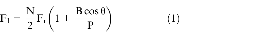
Figure 1 shows the configuration of a typical ball bearing consisting of an inner-race, ball, outer-race, and cage. The geometry of the ball bearing is presented in the cross-sectional view of Figure 1, where P, B, q are the pitch diameter, ball diameter, and contact angle between ball and inner race, respectively. Bearing faults can be classified into two categories: generalized-roughness faults and single-point faults. ¹³ The generalized-roughness is a noncyclic fault caused by improper lubrication, erosion, or pollution. Thus, there is no frequency dependency in the generalized-roughness fault.^13,18–20 The single-point fault is a localized fault generally caused by a small hole, pit, or missing material. The single-point fault generates periodic vibrations at specific frequencies when the bearing is rotated at a constant speed. ¹³ The frequency of a single-point fault in a ball bearing depends on the bearing geometry and rotational speed. The frequency characteristics of the single-points faults are represented as follows^21,22:

$${\mathrm{F}}_{\mathrm{I}}=\frac{\mathrm{N}}{2}{\mathrm{F}}_{\mathrm{r}}(1+\frac{\mathrm{B}\cos \mathrm{\theta }}{\mathrm{P}})$$

(1)

$${\mathrm{F}}_{\mathrm{O}}=\frac{\mathrm{N}}{2}{\mathrm{F}}_{\mathrm{r}}(1-\frac{\mathrm{B}\cos \mathrm{\theta }}{\mathrm{P}})$$

(2)

$${\mathrm{F}}_{\mathrm{B}}=\frac{\mathrm{P}}{2\mathrm{B}}{\mathrm{F}}_{\mathrm{r}}\{1-{\left(\frac{\mathrm{B}\cos \mathrm{\theta }}{\mathrm{P}}\right)}^2\}$$

(3)

Figure 1.

Configuration of ball bearing at the front and cross-sectional view across AA′.

where F_I, F_O, F_B, F_r, and N are inner-race fault frequency, outer-race fault frequency, ball fault frequency, rotor rotation speed, and the number of ball elements, respectively. As already mentioned, P, B, and q are the pitch diameter, ball diameter, and ball contact angle, respectively. For example, N, B, P, and q values of the 60/32 ball bearing are 10 ea, 5.8 mm, 47 mm, and 15°, respectively. Thus, the calculated fault frequencies of the bearing are as follows:

$${\mathrm{F}}_{\mathrm{I}}=5.596{\mathrm{F}}_{\mathrm{r}},{\mathrm{F}}_{\mathrm{O}}=4.404{\mathrm{F}}_{\mathrm{r}},\mathrm{and}{\mathrm{F}}_{\mathrm{B}}=3.994{\mathrm{F}}_{\mathrm{r}}$$

(4)

Convolutional neural network (CNN)

The diagnosis of bearing faults requires considerable expertise and engineering skills owing to its complex structure and various mechanical noises. However, deep CNNs have accomplished breakthroughs in processing images, video, speech, and audio. ²³ Various conventional deep learning models have used 1D numerical data as input (training) data. Moreover, 2D image data are converted into 1D numerical data, and then the converted 1D data are inputted into deep learning models. However, when 2D data are converted into 1D data, the multi-dimensional information in the 2D image is lost. CNN, a deep learning method, more effectively utilizes the spatial information of an image because it uses input data in 2D or 3D form. ²⁴

CNN is a type of feed-forward neural network that is constructed by two essential layers of a convolution layer (CL) and fully connected layer (FL), and an assistant layer of pooling layer (PL). A CL consists of multiple kernel matrix, k. Each kernel has trainable weight and bias and extracts local features from input data.^3,14,16,24 The output feature maps of kernels are used as input data for the next layer. The output feature maps of the lth layer can be described by the following equation ²⁵ :

$${\mathrm{x}}_{\mathrm{j}}^{\mathrm{l}}=\mathrm{f}({\sum }_{\mathrm{i}=1,\dots ,\mathrm{M}}{\mathrm{x}}_{\mathrm{i}}^{\mathrm{l}-1}{*\mathrm{k}}_{\mathrm{ij}}^{\mathrm{l}}+{\mathrm{b}}_{\mathrm{j}}^{\mathrm{l}}),\mathrm{j}=1,\dots ,\mathrm{N},$$

(5)

where ${\mathrm{k}}_{\mathrm{ij}}^{\mathrm{l}}$ represents the kernel of the jth filter connected to the ith input map of ${\mathrm{x}}_{\mathrm{i}}^{\mathrm{l}-1}$ , ${\mathrm{x}}_{\mathrm{j}}^{\mathrm{l}}$ is the jth output map, ${\mathrm{b}}_{\mathrm{j}}^{\mathrm{l}}$ is the bias corresponding to the jth filter, f is the activation function, and ∗ represents the convolutional operation. N feature maps can be obtained in this way.

The purpose of a PL, known as a sub-sampling layer is to reduce the spatial size of the feature maps produced by a CL. The PL merges similar local features into one; thus, the computation time and the parameters of the whole network are greatly reduced.^3,16 In addition, PLs are beneficial for preventing overfitting caused by training on a small training dataset. A pooling (sub-sampling) function can be described by ²⁵

$${\mathrm{x}}_{\mathrm{j}}^{\mathrm{l}}=\mathrm{f}\left({\mathrm{\beta }}_{\mathrm{j}}^{\mathrm{l}}\mathrm{down}({\mathrm{x}}_{\mathrm{j}}^{\mathrm{l}-1}+{\mathrm{b}}_{\mathrm{j}}^{\mathrm{l}})\right),\mathrm{j}=1,\dots ,\mathrm{M},$$

(6)

where down represents a pooling function and extracts the representative value in n × n region. ${\mathrm{b}}_{\mathrm{j}}^{\mathrm{l}}$ and ${\beta }_{\mathrm{j}}^{\mathrm{l}}$ are the additive bias and multiplicative bias corresponding to the jth filter, respectively. There are two types of pooling operations: max pooling and average pooling. A max pooling unit extracts the maximum value in a local patch on a feature map, and an average pooling unit computes the average of a local patch.^15,16

Following the feature extractions from CL and PL, FL is required to classify the features extracted from the input data. The “softmax” function, labeled as the normalized exponential function is generally used for feature classification. The sum of the output values from the softmax function is “1,” and each output value represents the possibility of the corresponding class. ¹⁵

Data acquisition and preprocessing

Acquisition of bearing vibration signal

In the experimental study, 60/32 ball bearings were used. Groove defects of 5 mm × 2 mm × 2 mm were formed on three different regions: inner-race, ball, and outer-race. Figure 2 shows the location and size of the artificial defects in the ball bearing. 10 defective bearings were prepared for each defect; thus 30 defective bearings were ready to test. To acquire the bearing vibration signal, the bearing test apparatus was constructed as shown in Figure 3. The experimental apparatus consisted of a 3-phase induction motor of 2HP, 60:1 speed reducer, magnetic coupling, 1:60 gearbox, and bearing housing integrated with an accelerometer. An accelerometer (352C34, PCB piezotronics, Inc.) was mounted perpendicular to the bearing housing, and the vibration signal was measured with a data acquisition board NI-9230 (National Instruments Co.).

Figure 2.

Location and size of artificial defects in ball bearing.

Figure 3.

Experimental setup for acquiring vibration signal from bearing housing.

In total, 40 bearings, including 30 defective bearings and 10 normal bearings, were used. For each bearing, the vibration data were collected for 980 s at a sampling frequency of 1 kHz. In addition, vibration data were measured at three different rotational speeds of 300, 600, and 1200 rpm. That is, collected data points for the specific rotational speed were 39,200,000 points: 980 s ×1000 Hz ×10 bearings ×4 kinds of bearings. For training the deep learning model, the collected data were separated every 10 s; thus, 3920 datasets (980 datasets/defect) were prepared at a specific rotational speed. Among the 3920 datasets, 3200 datasets were used as the training dataset, and the remaining 720 datasets were used as the validation datasets. The bearing fault detection accuracy was evaluated using specific datasets at each rotational speed, and also by using the mixed datasets of three rotational speeds. Therefore, when the mixed datasets were used, the number of training datasets were 9600: 3200 datasets with three different speeds. Figure 4(a) to (d) represent the 1D time-domain vibration data of normal, inner-race defective, ball defective, and outer-race defective bearings, respectively, obtained for 10 s under three different rotational speeds.

Figure 4.

1-D time-domain vibration numerical data obtained from the prepared ball bearings with: (a) normal condition, (b) defect in inner-race, (c) defect in ball, and (d) defect in outer-race.

The frequency characteristics of a single-point fault ball bearing depend on the rotor rotation speed, F_r, as shown in equations (1)–(3). When the bearing vibration data are mixed after collecting them at various ranges of rotor speed, the fault detection accuracy is dramatically reduced. Therefore, the previous works on deep learning-based bearing fault detection have used only the bearing vibration dataset acquired at a specific rotor rotation speed of 1125, ¹⁰ 1432, ¹⁸ and 2000 rpm. ¹³

In this study, the accuracy of the bearing fault detection was tested using specific datasets at a single rotational speed, and we also performed experiments using mixed datasets of three rotational speeds. The rotor rotation speeds of 300, 600, and 1200 rpm were considered. The frequency characteristics of a single-point fault ball bearing were calculated with equation (4). The obtained frequency ranges of F_r, F_I, F_O, and F_B were 5–20 Hz, 28–112 Hz, 22–88 Hz, and 20–80 Hz, respectively. Therefore, the frequency range of interest was determined to be less than 160 Hz.

Preprocessing of bearing vibration signal

In order to evaluate the effect of training data formats in deep learning models, two different deep learning models, MLP and CNN, were used in this study. As previously mentioned, six different training data formats of 1D time-domain numerical data, 1D FFT numerical data, 1D STFT numerical data, 2D time-domain image data, 2D FFT image data, and 2D STFT image (spectrogram) data were prepared. 1D numerical data and 2D image data were used as training data for the MLP and CNN classifiers, respectively.

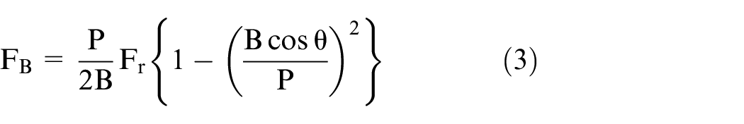
Figure 5 shows the preprocessing methods from 1D time-domain numerical data to other formats. The 1D time-domain numerical data consisted of 10,000 points for 10 s, as shown in Figure 5(a). 1D time-domain data were transformed to 1D FFT numerical data. Among the original 1D FFT numerical data with frequencies up to 500 Hz, the frequency range of less than 160 Hz was considered, as shown in Figure 5(b). Thus, the preprocessed 1D FFT numerical data had 1600 points. STFT was performed using a rectangular window of 1 s length and 94 % overlap in order to maintain a frequency resolution of less than 1 Hz. Consequently, 1D time-domain data of 10 s were changed into 1D SFTF data by 160 times of FFT. The size of each STFT dataset with 500 points was reduced to 160 points to make a 160 × 160 dataset. Figure 5(c) shows the STFT process using 1D time-domain data.

Figure 5.

Six different training data formats and data transformation processes: (a) 1-D time-domain numerical data of 10,000 points, (b) 1-D frequency-domain (fast Fourier transform, FFT) numerical data of 1,600 points, (c) 1-D frequency-domain (short-time fast Fourier transform, STFT) numerical data, (d) 2-D time-domain image data of 100 × 100 pixels, (e) 2-D FFT image data of 40 × 40 pixels, and (f) 2-D spectrogram (STFT) image data of 160 × 160 pixels.

Figure 5(d) to (f) represent preprocessing process of 2D image data from 1D numerical data in detail. After normalizing from 0 to 1 by the maximum value, 10,000 points in 1D time-domain numerical data were consecutively arranged as 2D image data of 100 ×100 pixels, as shown in Figure 5(d). The conversion method used the flatten 2D matrix method as the data arrangement method and arranged in the reverse order of the matrix. Similarly, FFT numerical data in Figure 5(b) were converted into 2D FFT image data of 40 ×40 pixels represented in Figure 5(e), and 2D spectrogram image data of 160 ×160 pixels in Figure 5(f) was also constructed. Consequently, the FFT data in Figure 5(b) and (e) had a resolution of 0.1 Hz and a single transformed result, while the STFT data in Figure 5(c) and (f) had a resolution of 1 Hz and multiple transformed results.

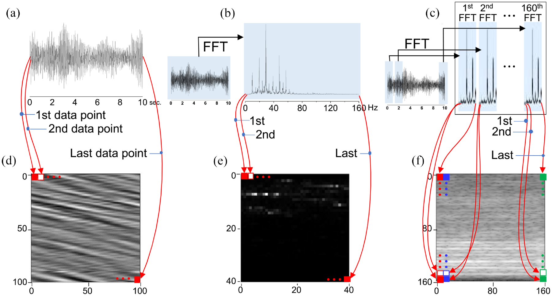
Figure 6(a) to (d) represent the 2D time-domain image data of normal, inner-race defective, ball defective, and outer-race defective bearings, respectively. Figures 7 and 8 show the 2D FFT and 2D spectrogram image data, according to different rotor rotational speeds.

Figure 6.

2-D time-domain image data converted from 1-D numerical data shown in Figure 4: (a) normal bearing, (b) inner-race defective, (c) ball defective, and (d) outer-race defective bearing.

Figure 7.

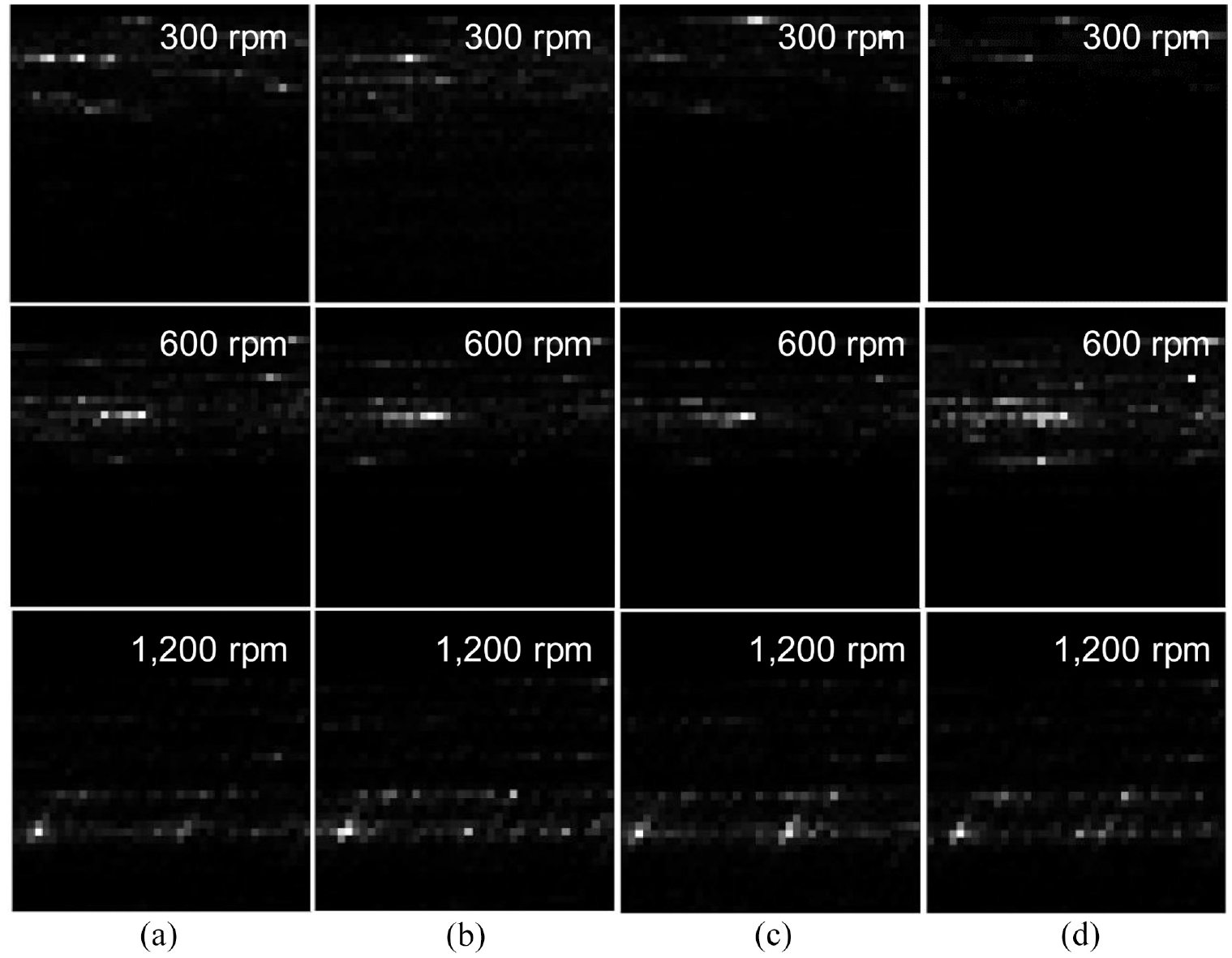
2-D fast Fourier transform image data converted from 1-D fast Fourier transform data: (a) normal, (b) inner-race defective, (c) ball defective, and (d) outer-race defective bearing.

Figure 8.

2-D spectrogram image data converted from 1-D short-time Fourier transform data: (a) normal, (b) inner-race defective, (c) ball defective, and (d) outer-race defective bearing.

Deep learning models

We considered two different deep learning models and three different training data formats for each deep learning model. Figure 9 presents the architecture of the MLP and CNN models. As shown in Figure 9(a), the input data format was a 1D vector and its size was dependent on the training data size. The hidden layer consisted of two layers, and the number of neurons was empirically set to 10,000 in each hidden layer. The ReLU function was used as the activation function, and the softmax function was used for feature classification in the last layer.

Figure 9.

Models of deep learning for the mixed rotational speed dataset: (a) multi-layer perception and (b) convolutional neural network.

Figure 9(b) shows the inner structures of the CNN-based model, and input data format of the CNN was 2D image data. In this work, 160 kernels of 3 ×3 size and stride 1 with padding to maintain the dimensions of the output as those of the input were used in the CL. Kernel weights were initialized by Xavier uniform initialization method. The ReLU function was used as activation function. Following CL, max pooling with 2 ×2 filter and stride 2 was performed in the PL. After pooling, the input image size is reduced to a quarter of the original training image size. The CNN was constructed using three CL and PL combination layers, a flattened layer, an FL with 160 neurons, and a softmax layer. In this work, a 30% dropout rate was added between the CL and PL to reduce the overfitting. ²⁶

Besides the input data format, several hyperparameters of the deep learning model were changed and evaluated, because hyperparameters have significantly affected the prediction accuracy. ²⁷ In MLP model, the effect of the number of hidden layers and neurons were investigated. Two to four hidden layers with 5000 neurons combination, and 1000 to 10,000 neurons with two hidden layers combination were used. In the case of CNN model, the number of CLs, the number and size of kernels were examined. The impact of hyperparameters was evaluated by varying the number of CLs from 2 to 12, the number of kernels from 8 to 256, and kernel size from 3 ×3 to 8 ×8. In this investigation, mixed dataset was only considered as input dataset.

The Adam optimizer was used in both MLP and CNN deep learning models, and the learning rate was 0.001, and the momentum factor was set to 0.9 for the first momentum and 0.999 for the second momentum (both the learning rate and the momentum value used the keras adam optimizer default value). And when all algorithms are used, the mini batch size is set to 100, and the attenuation rate is not set.

Results and discussions

Experiments were classified into two major groups: single rotational speed and mixed rotational speed. A single rotational speed experiment consisted of four input classes and four output classes including normal, inner-race defective, ball defective, and outer-race defective classes. In contrast, a mixed rotational speed experiment had 12 input classes and 12 output classes since the bearing vibration data were acquired at three different rotational speeds, as shown in Figure 9(a). For each rotational speed, 3200 datasets among 3920 datasets related to four input classes were used as the input training dataset. In the mixed rotational speed experiment, 9600 datasets were too abundant to be used as inputs; thus, the mixed 9600 datasets were randomly divided into three groups. Then, randomly mixed 3200 datasets related to 12 input classes were used as the input training dataset.

Table 1 presents the test accuracy according to the deep learning models and training data format. The 1D time-domain and FFT numerical data format in the MLP model showed 100% accuracy at each rotation speed (four input and four output classes). However, when all the vibration data obtained at three different rotation speeds were mixed together (12 input and output classes), the test accuracy was dramatically decreased to less than 50% for the 1D time-domain data. Furthermore, 1D STFT numerical data did not work properly with MLP model, as shown in Table 1. Consequently, the 1D numerical data format was suitable for bearing fault detection of the unmixed single rotation speed, and the FFT numerical data among 1D numerical data showed higher test accuracy in the MLP model.

Table 1.

Prediction accuracy of validation test according to deep learning model, training data format, and training dataset composition (MLP: 2 hidden layers, 10,000 neurons, CNN: 3 × 3, 160 kernels, 2 convolution layers).

Classes		Prediction accuracy
Deep Learning Model		Multi-layer perceptron			Convolutional neural network
Rotational speed		Data format
		1D numerical data format			2D image data format
		Time data	FFT data	STFT data	Time data	FFT data	STFT data
Single dataset (4 output)	300 rpm	100%	100%	96.53%	94.53%	95.75%	97.70%
	600 rpm	100%	100%	92.15%	88.30%	94.65%	94.75%
	1200 rpm	100%	100%	80.58%	85.63%	92.58%	94.30%
Mixed dataset (12 output)		47.20%	90.67%	78.74%	92.07%	99.21%	99.06%

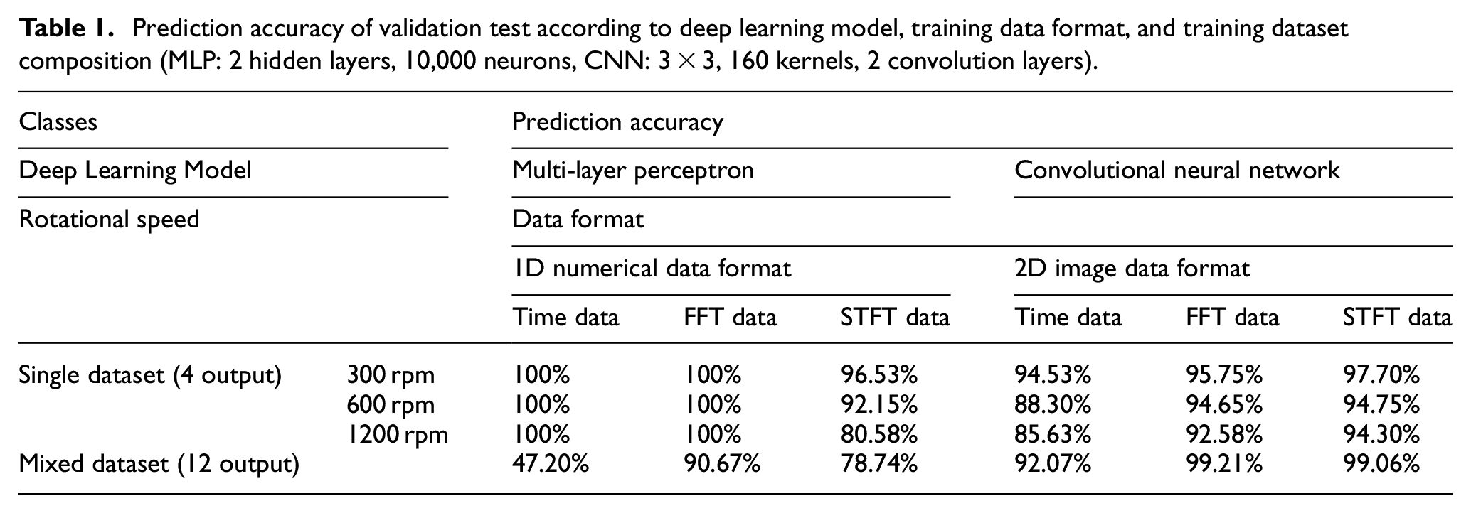
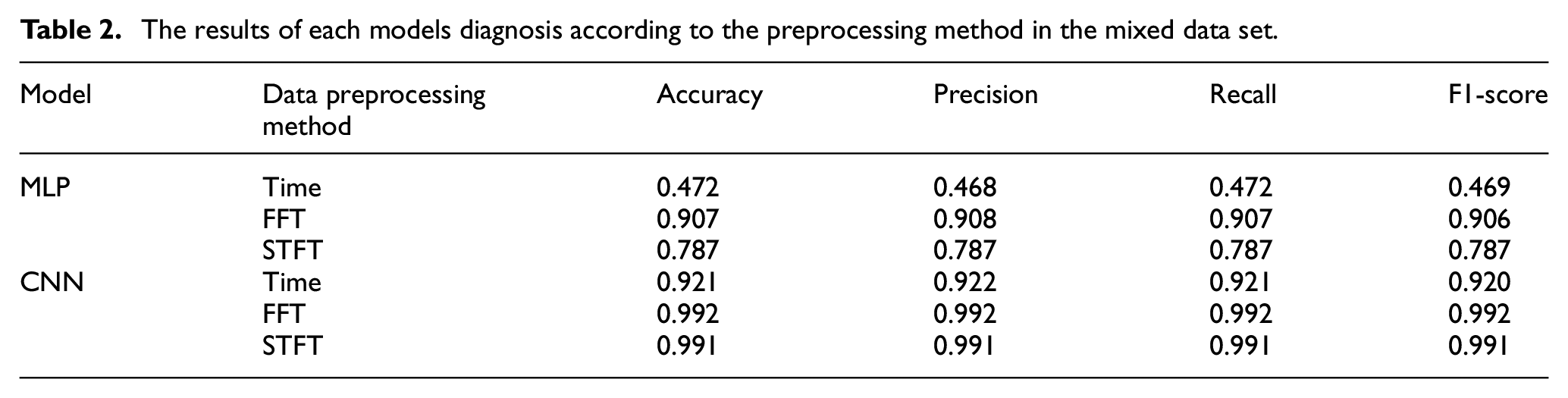
Table 2 shows the diagnostic results of precision, accuracy, recall, and F1-Score of each model according to the preprocessing method of the mixed data set. In order to create a model suitable for classifying/diagnosing machine failure, “reliable data acquisition” and “appropriate evaluation criteria” are required. Therefore, in order to construct a more suitable model/classification model, F1-score, an evaluation criterion that considers precision and recall, was used. Considering the F1-score and accuracy, it is better to use the CNN model rather than the MLP model.

Table 2.

The results of each models diagnosis according to the preprocessing method in the mixed data set.

Model	Data preprocessing method	Accuracy	Precision	Recall	F1-score
MLP	Time	0.472	0.468	0.472	0.469
	FFT	0.907	0.908	0.907	0.906
	STFT	0.787	0.787	0.787	0.787
CNN	Time	0.921	0.922	0.921	0.920
	FFT	0.992	0.992	0.992	0.992
	STFT	0.991	0.991	0.991	0.991

2D time-domain image data were less accurate with the CNN model, whereas the 2D frequency-domain image data of FFT and STFT showed a test accuracy of more than 92% compared to 2D time-domain image data. Time-domain data were more suitable for the MLP model than the CNN model. For the dataset of each unmixed rotational speed, as the rotational speed increased, the test accuracy slightly decreased. However, when all the bearing vibration data were mixed together, the CNN model worked well with 2D frequency-domain image data. For the case of 12 input and 12 output classes (mixed data), the CNN model with FFT and STFT image data provided a test performance with at least 99% accuracy. The test accuracies of the 2D time-, 2D FFT-, and 2D STFT-image data format in the CNN model were 92.07%, 99.21%, and 99.06%, respectively.

At the beginning of this study, the characteristic frequencies of a single-point fault ball bearing as described in equation (4) were overlapped as the rotor rotational speed was increased from 300 to 1200 rpm; thus, a deep learning model for the mixed dataset might make incorrect predictions or the different rotor rotational speed datasets may confuse the model. Hence, the MLP and CNN models present completely different results. Figure 10 represents the confusion matrix of the validation test results for the mixed training datasets. The wrong prediction mainly occurred within the same rotational speed dataset (red-dotted rectangular box in Figure 10), not across different rotational speed datasets. In particular, incorrect predictions were mostly made at a high rotational speed of 1200 rpm rather than 300 rpm in the MLP model. In the CNN model, incorrect predictions were only 1200 rpm among the mixed rotation speeds.

Figure 10.

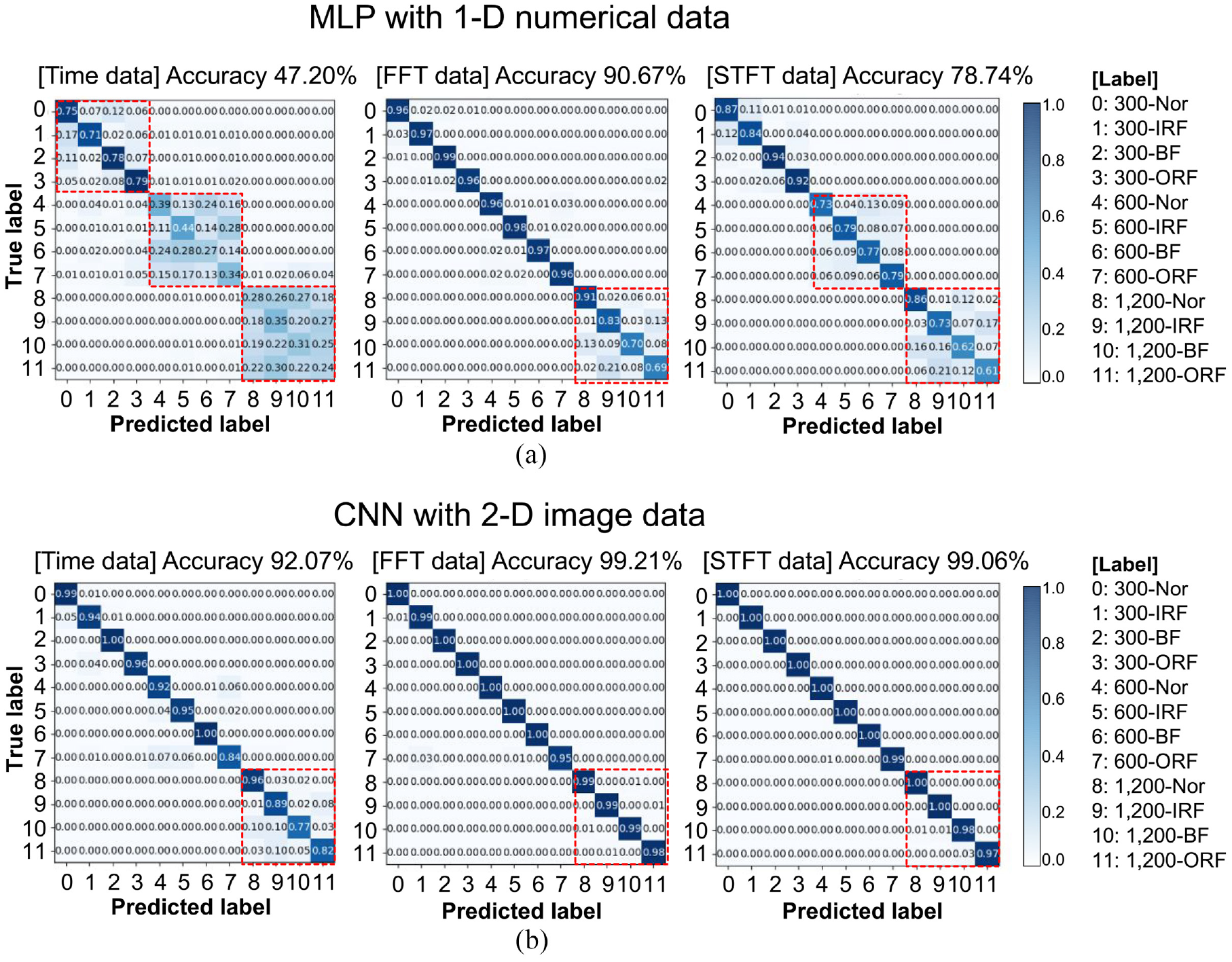
Confusion matrix of validation test results for the mixed training datasets of three different rotational speeds. Labels of 0–11 mean: 300 rpm normal (Nor), 300 rpm inner-race fault (IRF), 300 rpm ball fault (BF), 300 rpm outer-race fault (ORF), 600 rpm Nor, 600 rpm IRF, 600 rpm BF, 600 rpm ORF, 1200 rpm Nor, 1200 rpm IRF, 1200 rpm BF, and 1200 rpm ORF, respectively. (a) MLP with 1-D numerical data and (b) CNN with 2-D image data.

Figure 11 presents the prediction accuracies according to various hyperparameters for each input data format. In the MLP model, the number of hidden layers had no impact on the prediction accuracy, while the number of neurons significantly affected the prediction accuracy, as shown in Figure 11(a). To improve the prediction accuracy, it is recommended to use as many neurons as possible within computing power.

Figure 11.

The effect of hyperparameters in MLP and CNN models on the prediction accuracy for the mixed training datasets of three different rotational speeds: (a) the impact of the number of hidden layers and neurons in MLP model, (b) the impact of the number of convolution layers in CNN models, and (c) the impact of the number and size of kernel in CNN models. Inside the red-line, the prediction accuracy was higher than 95%.

In the CNN model, when the number of CLs was increased, the prediction accuracy was dramatically decreased for all input data formats. As shown in Figure 11(b), two or three CLs were enough for high prediction accuracy, and FFT-image data showed less standard deviation in five times prediction test rather than time- and STFT-image data. On the other hand, the number and size of kernel have significantly affected test accuracy depending on the input data format. Figure 11(c) shows the prediction accuracy contour graph according to the number and size of kernels for each input data format. For the time-image data, the prediction was improved, as the number and size of kernels increased. More computing power is required for the time-image data in order to get higher prediction accuracy. In the case of FFT-image data, test accuracy exceeded 99% for all 36 kernel combinations; thus red boundary line (>95%) in Figure 11(c) covers all contours area. However, STFT-image data represented several local maximum and minimum values in the prediction accuracy; thus had low average and large standard deviation in the prediction accuracy of 86.5% and 6.7%. STFT-image data was very sensitive to kernel parameters.

Summary and conclusion

This paper presents the effect of training data formats in deep learning on the accuracy of ball bearing fault detection. In order to obtain the machine learning data for ball bearing fault detection, three different defects were artificially created on the ball bearing, and then acceleration-based vibration data were acquired with a sampling frequency of 1 kHz at the rotation speeds of 300, 600, and 1200 rpm. For each rotor rotational speed, 800 datasets were used as the training data, and the prediction accuracy was verified using 180 datasets. For the single rotor rotational speed, four input and output classes with one normal and three different defective bearings were trained and tested. Twelve input and output classes were also investigated by mixing all the vibration data obtained from three different speeds. Six different training data formats were considered. For the MLP model, 1D time-domain numerical data, 1D FFT numerical data, and 1D STFT numerical data formats were tested. 2D time-domain image data, 2D FFT image data, and 2D STFT spectrogram image data formats were used in the CNN model. Consequently, the 1D numerical data format of time data and FFT data in the MLP model presented 100% prediction accuracy for four input and four output classes, while the 1D numerical data format showed poor prediction accuracy in the 12 input and 12 output classes. In particular, the 1D time data prediction accuracy was less than 50% for the mixed data. In contrast, 2D image data formats in the CNN model worked effectively for the mixed vibration data: 12 input and 12 output classes. The 2D FFT- and 2D STFT-image data formats presented 99.21% and 99.06% prediction accuracy, respectively. Experimental results imply that the training data formats significantly affect the prediction accuracy in the same deep learning model; thus, signal preprocessing needs to be performed more carefully. In addition, the number of neurons was more important rather than that of hidden layers in the MLP model, while both the input data format and hyperparameters significantly affected the prediction accuracy in the CNN model. Consequently, the selection of FFT-image data as the input data format is more suitable because FFT-image data is less sensitive to hyperparameters such as kernel and convolution layer and shows higher test accuracy, at least 99% for the bearing fault detection. It is applied to the fault condition monitoring system of all low-speed rotating machinery, such as the rotor of a wind turbine generator and medical equipment, and it is judged that damage caused by bearing defects can be prevented in advance.