Penalized K-Means Clustering: Another Look at Its Statistical Properties

Abstract

Unsupervised learning is a major class of machine learning techniques where response information is missing or unavailable. Among these techniques, clustering plays a central role by grouping objects based on a chosen similarity measure. K-Means is one of the most established and widely used clustering methods, known for its simplicity and computational efficiency. For continuous data, K-Means performs well when the number of clusters $(K)$ is known and correctly specified. However, it faces convergence and overfitting challenges when $K$ is unknown. These issues stem from K-Means’ objective function, which monotonically decreases as the number of clusters increases—leading to a tendency to overfit. In this article, we propose an augmented K-Means algorithm that introduces a penalized version of the standard K-Means objective, designed to guard against overfitting and promote model parsimony when $K$ is unknown. We establish key optimality properties of both the traditional K-Means loss function and the proposed penalty term. Extensive simulation studies on benchmark datasets demonstrate the improved performance of the proposed method, including accurate identification of the true number of clusters. Extensive simulation studies on benchmark datasets demonstrate the improved performance of the proposed method, including accurate identification of the true number of clusters. Additionally, we apply our approach to the clustering of globular galaxy datasets—an example of truly large-scale (“Big”) data—to further illustrate its effectiveness.

1. Introduction

Unsupervised learning problems arise when there is no available information about the response or outcome variable, yet it remains necessary to draw inferences from the observed input features. Clustering is a core task in this setting, aiming to partition the data into distinct groups based on shared characteristics among the features. This process helps reveal the natural structure of the data, offering insights that are both meaningful and applicable across a wide range of domains. A variety of clustering techniques exist, differing K-Means in how they segment the data space into clusters of observations. Broadly speaking, the goal is to ensure that observations within a cluster are more similar to each other, while observations in different clusters are more dissimilar—according to a chosen similarity or distance measure. Clustering mechanisms can be partitioned K-Means into two subcategories with respect to mechanism of forming clusters, namely,

Hierarchical clustering: Objects are clustered in a top-down or bottom-up hierarchy based on a chosen distance metric and linkage function, resulting in a tree-like structure. Examples include Agglomerative clustering and Divisive clustering.

Connectivity-based clustering: Each cluster is represented by a “center” and is constructed via minimizing the distance metric between cluster objects to the center, e.g., K-Means clustering, Medoid based clustering etc.

Each of these methods can be implemented using either a deterministic approach or a probabilistic, model-based framework. Both approaches have their own advantages and disadvantages, and their popularity largely depends on the application domain (e.g., social sciences, marketing, genetics, infectious disease hotspots, astronomy, etc.) as well as the ease of interpretability within that domain. Recent developments in clustering includes density-based approaches (Ester et al., 1996), graph-based/spectral clustering (Shi & Malik, 2000), convex clustering (Chi & Lange, 2015; Radchenko & Mukherjee, 2017; Tan & Witten, 2015) etc. In this article, we are focusing on the Connectivity-based clustering mechanism, especially, K-Means clustering which depends upon the choice of the $K$ or cluster centers, and a distance metric. For continuous data, the Euclidean norm is the most popular, albeit, other distance measures (e.g. $L_1$ , $L_2$ etc.) are also explored and in turn, each norm imposes different probability distribution in case one want to exploit the duality between loss and probability distribution. K-Means with Euclidean norm is not only simple to implement and interpret but also has a strong connection with Gaussian mixture models. For a fixed cluster number $K$ theoretical results exist showing the consistency of K-Means under various regularity conditions (MacQueen et al., 1967; Pollard, 1981). Nevertheless, a fundamental problem with this type of clustering is the choice of cluster number as $K$ is often unknown. In this situation there is a tendency of mixture models to overfit on real data (Nguyen, 2013). Several works also have addressed this issue through various criteria for choosing optimal cluster numbers including “model-free” approach. Fraley and Raftery (1998) addressed the problem of cluster choice for model-based clustering via BIC criterion, Sugar and James (2003) optimized the cluster number of K-Means through distortion-based measure, Fang and Wang (2012) introduced clustering stability-based idea for choosing optimum cluster number, de Amorim and Hennig (2015) utilized feature rescaling to achieve optimal clusters in K-Means. In this paper, we make four key contributions. First, we theoretically prove that when $K$ is unknown, the K-Means algorithm minimizes the underlying loss function as $K\to N$ , where $N$ is the number of data points. This represents the most complex model possible and ultimately defeats the purpose of clustering. Second, to address this overestimation issue, we propose a penalty function on the number of clusters, which is minimized when $K=1$ , thus encouraging the simplest model. Third, we combine the loss and penalty functions to develop an augmented, penalized version of K-Means, and we study its properties under various tuning parameter selection criteria. Fourth, we address another computational limitation of standard K-Means: its non-recursive optimization. Specifically, for each value of $K$ , K-Means restarts the optimization from scratch, without leveraging the solution from the previous iteration. This leads to non-monotonicity in the clustering solution with respect to $K$ , as the algorithm explores multiple potentially suitable values. Our modified K-Means algorithm improves this by reusing the solution from the previous step, allowing each optimization for a given $K$ to build on the result from $(K-1)$ -th stage clustering. This not only accelerates computation but also makes the method scalable and manageable for truly massive datasets (as $N\uparrow$ in our example).

The rest of the article is organized as follows. In Section 2, we discuss some issues with standard K-Means clustering and propose remedies to address these problems. Section 3 presents modifications to the K-Means algorithm for the automatic detection of the number of clusters in a dataset. The optimization methodology and the method for tuning parameter selection are elaborated in Sections 4 and 5, respectively. Simulation studies and applications to a real data problem are provided in Sections 6 and 7, respectively. Finally, Section 8 offers concluding discussion with future directions. For the sake of brevity, all proofs have been provided in the supplementary material.

2. Properties of K-Means Clustering

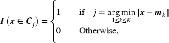
At first we will concentrate on some convergence properties of standard K-Means clustering problem. Assume the data in hand is $N\times p$ matrix $\mathit{X}=({\mathit{x}}_1,\dots ,{\mathit{x}}_N)$ , each ${\mathit{x}}_i$ is a $p$ -dimensional vector. In any clustering mechanism, we partition the data matrix $\mathit{X}$ into $K$ possible clusters with ${\mathcal{C}}_j\mathrm{\forall }j=1,\dots ,K$ is an assignment set. For center-based clustering, a data point $\text{``}{\mathit{x}}^{″}$ is part of cluster ${\mathcal{C}}_j$ if

$$\mathit{I}(\mathit{x}\in {\mathcal{C}}_j)=\{\begin{array}{ll}1& \text{if}j=\underset{1\le k\le K}{\arg min}\Vert \mathit{x}-{\mathit{m}}_k\Vert \\ 0& \text{Otherwise},\end{array}$$

where $\Vert .\Vert$ is Euclidean norm and ${\mathit{m}}_j$ is the center for cluster ${\mathcal{C}}_j$ . Particularly, In K-Means clustering, the main idea is to choose $K$ centers and update them in such a fashion so that the sum of distances of all points from their respective cluster center is minimum. Therefore the optimization problem for K-Means solves,

$$\underset{{\mathit{m}}_k\in {\mathbb{R}}^p,1\le k\le K}{\arg min}{\mathit{L}}_K(\mathit{X},\mathit{M})=\underset{{\mathit{m}}_k\in {\mathbb{R}}^p}{\arg min}\underset{i=1}{\sum ^N}\underset{1\le k\le K}{\arg min}\Vert {\mathit{x}}_i-{\mathit{m}}_k{\Vert }^2=\underset{{\mathit{m}}_k\in {\mathbb{R}}^p}{\arg min}\underset{i=1}{\sum ^N}\underset{k=1}{\sum ^K}\mathit{I}({\mathit{x}}_i\in {\mathcal{C}}_k)\Vert {\mathit{x}}_i-{\mathit{m}}_k{\Vert }^2$$

with $\sum _{k=1}^K\mid {\mathcal{C}}_k\mid =N$ where $\mid .\mid$ represents the cardinality of a set and $\mathit{M}=({\mathit{m}}_1,\dots ,{\mathit{m}}_K)$ is the $K\times p$ matrix of cluster centers. Theoretically $1\le K\le N$ , however in most practical situations $K<<N$ and chosen as the maximum plausible cluster number. It is well known that the above optimization works well for known for fixed $K$ (MacQueen et al., 1967; Pollard, 1981). However, if the value of the actual cluster number $\text{``}{K}^{″}$ is unknown and treated as a parameter with $K\in \{1,2,\dots ,N\}$ , the above loss function will yield a trivial minimum at $K=N$ i.e., each observation is its own cluster center and we will have $\underset{{\mathit{m}}_k\in \mathbb{R}}{\arg min}{\mathit{L}}_K(\mathit{X},\mathit{M})=0$ , which is the lowest possible value of the K-Means objective function. The same is true for a slightly more generalized K-Means loss function,

$$\underset{{\mathit{m}}_k\in {\mathbb{R}}^p,1\le k\le K}{\arg min}{\mathit{L}}_K(\mathit{X},\mathit{M})=\underset{{\mathit{m}}_k\in {\mathbb{R}}^p}{\arg min}\underset{i=1}{\sum ^N}\underset{k=1}{\sum ^K}\mathit{I}({\mathit{x}}_i\in {\mathcal{C}}_k)\Vert {\mathit{x}}_i-{\mathit{m}}_k\Vert$$

(1)

where the distance functions $\Vert .\Vert$ is any norm following these properties,

• $\Vert \mathit{x}\Vert \ge 0\mathrm{\forall }\mathit{x}\in {\mathbb{R}}^N$ and attains 0 only if $\mathit{x}=0$ (non-negative property),

• $\Vert \lambda \mathit{x}\Vert =\mid \lambda \mid \Vert \mathit{x}\Vert \mathrm{\forall }\mathit{x}\in {\mathbb{R}}^N\text{and}\lambda \in \mathbb{R}$ (homogeneous property),

• $\Vert \mathit{x}+\mathit{y}\Vert \le \Vert \mathit{x}\Vert +\Vert \mathit{y}\Vert \mathrm{\forall }\mathit{x},\mathit{y}\in {\mathbb{R}}^N$ (triangular inequality).

Note, Euclidean norm is a special case and in fact for any $L_p,(p\ge 1)$ norm is also going satisfy these conditions. The aforementioned properties of the distance function are the necessary foundations for the proofs of the following propositions and theorems. Next, we will propose a general result on distance norm following the aforementioned properties, for any three p-dimensional points. Proposition 1

For three points ${\mathit{v}}_1,{\mathit{v}}_2\text{and}{\mathit{v}}_3$ , we have

If ${\mathit{v}}_3$ has the convex form ${\mathit{v}}_3=\theta {\mathit{v}}_1+(1-\theta ){\mathit{v}}_2$ for some $\theta \in [0,1]$ then $\Vert {\mathit{v}}_1-{\mathit{v}}_3\Vert +\Vert {\mathit{v}}_2-{\mathit{v}}_3\Vert =\Vert {\mathit{v}}_1-{\mathit{v}}_2\Vert$ .

For all other ${\mathit{v}}_3$ , $\Vert {\mathit{v}}_1-{\mathit{v}}_2\Vert \le \Vert {\mathit{v}}_1-{\mathit{v}}_3\Vert +\Vert {\mathit{v}}_2-{\mathit{v}}_3\Vert$ .

Proof.

The proof is trivial from homogeneous and triangular inequality property of distance function under any norm.

The proposition can be extended for any convex set $\mathit{A}$ containing a set of points ${\mathit{x}}_i\in \mathit{A}\mathrm{\forall }i=\{1,2,\dots \}$ . In the next Lemma, we propose a result on the optimization under any convex set. Lemma 1

For a convex set $\mathit{A}$ , the optimizer of $\underset{u\in \mathit{A}}{min}\sum _i\Vert {\mathit{x}}_i-u\Vert$ for all ${\mathit{x}}_i\in \mathit{A}$ will be unique.

Lemma 1 states that, within a convex set, the point that minimizes the sum of distances to all other points in the set is unique. Leveraging this result, one can establish the uniqueness of the solution to a given loss function under the assumption of convexity. Together, this lemma and the preceding proposition provide the foundational tools necessary to prove the next two theorems, demonstrating that the solution to the optimization problem under consideration in K-Means (in equation 1) is indeed unique when the convexity condition is satisfied. It is to be noted that, if ${\mathit{m}}_k$ is the cluster center of cluster ${\mathcal{C}}_k$ then we consider center as, ${\mathit{m}}_k=\sum _{i\in {\mathcal{C}}_k}{\theta }_i{\mathit{x}}_i\text{ with }\sum _{i\in {\mathcal{C}}_k}{\theta }_i=1$ , i.e., each cluster center can be represented as a convex combination of the points in the cluster. The characteristic of solution to the K-Means optimization described in equation (1) with unknown $K$ is described in the next theorem. Theorem 1

The loss function ${\mathit{L}}_K(\mathit{X},\mathit{M})$ is a monotone decreasing function in $K\in \{1,\dots ,N\}$ and reaches its minima at $K=N$ , for each ${\mathit{m}}_k\in {\mathcal{C}}_k\mathrm{\forall }k\in \{1,\dots ,K\}$ .

Remark

Theorem 1 shows that unless we specify the cluster number of a K-Means, the underlying optimization problem denoted by ${\mathit{L}}_k(\mathit{X},\mathit{M})$ will always encourage more complex model with high number of clusters. In other words, given $\hat{\mathit{M}}$ as a $k\times p$ cluster center matrix, if we introduce another cluster center by optimizing equation (1) to get $(k+1)\times p$ cluster center matrix ${\hat{\mathit{M}}}^{*}$ , then it is guaranteed to hold ${\mathit{L}}_{k+1}(\mathit{X},\hat{\mathit{M}})\le {\mathit{L}}_k(\mathit{X},{\hat{\mathit{M}}}^{*})$ . Thus, the naive K-Means for an unknown number of clusters is an ill-posed problem, which necessitate a penalty parameter to guard against it.

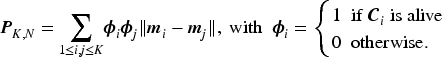
It is evident from Theorem 1, K-Means with unknown $K$ will always encourage a large number of clusters and the need to regularize the optimization function in equation (1) to prevent overfitting. The penalty term chosen for this work is,

$$\begin{array}{r}{\mathit{P}}_{K,N}=\sum _{1\le i,j\le K}{\mathit{\varphi }}_i{\mathit{\varphi }}_j\Vert {\mathit{m}}_i-{\mathit{m}}_j\Vert ,\text{ with }{\mathit{\varphi }}_i=\{\begin{array}{l}1\text{if}{\mathcal{C}}_i\text{is alive}\\ 0\text{otherwise}.\end{array}\end{array}$$

Since the contribution of the penalty term is only for the clusters that are alive i.e., if both ${\mathit{\varphi }}_i$ and ${\mathit{\varphi }}_j$ is 1, therefore we can reduce the penalty as

$${\mathit{P}}_{K,N}=\sum _{1\le i,j\le K}\Vert {\mathbf{\text{m}}}_i-{\mathbf{\text{m}}}_j\Vert .$$

(2)

It is to be noted here that ${\mathit{P}}_{K,N}$ has a trivial minimum at $K=1$ since all the observations fall within a single cluster and will have higher values as $K\uparrow$ . In a sense, it behaves exactly oppositely to that of the loss function in equation (1). This type of penalty function using the Gaussian norm was first considered by our group in Ghosh and Dey (2009). Later Hocking et al. (2011) considered a $L_1$ and Lindsten et al. (2011) considered a $L_p$ penalized version of it. Though intuitively this makes sense, but none of these developments are without any direct proof about the properties of the considered penalty. In Theorem 2 we study the behavior of the penalty ${\mathit{P}}_{K,N}$ as a function of the $K$ . Theorem 2

The penalty ${\mathit{P}}_{K,N}=\sum _{1\le i,j\le K}\Vert {\mathit{m}}_i-{\mathit{m}}_j\Vert$ is a monotone increasing function in $K\in \{1,\dots ,N\}$ and attains maximum at $K=N$ , under the assumption that each cluster center ${\mathit{m}}_k$ lies in the convex hull $C_k$ of the $k^{th}$ cluster $\mathrm{\forall }k\in \{1,\dots ,K\}$ .

Remark

Theorem 2 states that when the number of clusters varies, the proposed penalty when minimized will always favor the simplest model, i.e., one in which all points belong to a single cluster. Furthermore, as we increase the number of clusters from $K$ to $K+1$ in the same $p$ -dimensional feature space, the corresponding penalty values satisfy ${\mathit{P}}_{k,N}\le {\mathit{P}}_{k+1,N}$ and the penalty reaches its maximum when $K=N$ . This behavior of the penalty term, when combined with the loss function in equation (1), provides the necessary balance for selecting the optimal value of $K$ .

In the next section, we describe an augmented versus of K-Means clustering which combines the loss (in equation (1)) and penalty (in equation (2)) in a regularized framework. The monotone nature of both terms ensures parsimonious model selection, with appropriately chosen regularization parameter.

3. Reformulation of K-Means Clustering

The augmented version of the K-Means problem solves following optimization problem,

$$\underset{{\mathit{m}}_k\in {\mathbb{R}}^p}{\arg min}\underset{i=1}{\sum ^N}\underset{k=1}{\sum ^K}\mathit{I}({\mathit{x}}_i\in {\mathcal{C}}_k)\Vert {\mathit{x}}_i-{\mathit{m}}_k\Vert +\lambda \sum _{1\le i,j\le K}\Vert {\mathit{m}}_i-{\mathit{m}}_j\Vert .$$

(3)

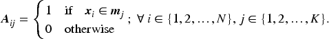
The first part of the optimization governs the assignment of data points to clusters, while the second part constrains the number of cluster centers. Thus, with an appropriate choice of the tuning parameter $\lambda (\in [0,\mathrm{\infty }))$ , the augmented K-Means simultaneously optimizes both the cluster centers and the number of clusters. Next, we reformulate the optimization problem in equation (3) using matrix notation, where ${\mathit{A}}_{N\times K}$ denotes cluster assignment matrix

$${\mathit{A}}_{ij}=\{\begin{array}{ll}1& \text{if}{\mathit{x}}_i\in {\mathit{m}}_j\\ 0& \text{otherwise}\end{array};\mathrm{\forall }i\in \{1,2,\dots ,N\},j\in \{1,2,\dots ,K\}.$$

Each element of $\mathit{A}$ denotes the cluster assignment of observation ${\mathit{x}}_i$ , whereas $\mathit{M}$ is the $K\times p$ matrix of cluster centers. Thus equation (3) can be reformulated as,

$$\underset{{\mathit{m}}_k\in {\mathbb{R}}^p,1\le k\le K}{\arg min}\underset{i=1}{\sum ^N}\Vert {\mathit{x}}_i-{\mathit{A}}_{i.}\mathit{M}\Vert +\lambda \sum _{1\le i,j\le K}\Vert {\mathit{m}}_i-{\mathit{m}}_j\Vert ,$$

(4)

where ${\mathit{A}}_{i.}$ denotes the $i$ -th row of $\mathit{A}$ . Note, that the optimization problem stated above is fairly general and should work for any choice of distance norm, though, for the K-Means algorithm with continuous features, the natural choice is Euclidean norm or it squared version. It should be also noted different non-concave norms can be also chosen separately for loss and penalty terms as it is done in the regression context for LASSO type problems (Bach et al., 2012) and clustering via regression-based approach Wu et al. (2016). Albeit, the different norms in Loss and Penalty will lead to differential contraction (Grossmann & Winkler, 2013) which needs to be studied further theoretically, this may also be dictated by the nature of feature space (e.g., discrete, continuous, Boolean, etc.) based on which clustering is performed. For this work, we stick to squared error loss (or square of Euclidean norm) due to its acceptability and ease of computation. Under that we have the following optimization problem,

$$\underset{{\mathit{m}}_k\in {\mathbb{R}}^p,1\le k\le K}{\arg min}\underset{i=1}{\sum ^N}\Vert {\mathit{x}}_i-{\mathit{A}}_{i.}\mathit{M}{\Vert }^2+\lambda \sum _{1\le i,j\le K}\Vert {\mathit{m}}_i-{\mathit{m}}_j{\Vert }^2.$$

(5)

The loss function in above equation can be rewritten as $(\mathit{X}-\mathit{A}\mathit{M}{)}^T(\mathit{X}-\mathit{A}\mathit{M}).$ Whereas it can be easily shown that the difference between cluster centers can be written as, ${\mathit{m}}_i-{\mathit{m}}_j={\mathit{M}}^T({\mathit{e}}_i-{\mathit{e}}_j)$ where ${\mathit{e}}_i$ is a $k$ -dimensional vector of zero’s with $1$ at $i$ -th position. Thus our optimization problem of 5 boils down to

$$\underset{\mathit{M}\in {\mathbb{R}}^{k\times p},1\le k\le K}{\arg min}{(\mathit{X}-\mathit{A}\mathit{M})}^T(\mathit{X}-\mathit{A}\mathit{M})+\lambda \sum _{1\le i,j\le K}{({\mathit{e}}_i-{\mathit{e}}_j)}^T\mathit{M}{\mathit{M}}^T({\mathit{e}}_i-{\mathit{e}}_j).$$

(6)

Note that we still need to pre-specify a value of $K$ (as an upper limit) for the optimization in equation (6). Given this value, our algorithm is capable of selecting the optimal number of clusters within the range $[1,K]$ . The most liberal choice of $K$ is the total number of samples or $N$ . However, this choice comes with a potential drawback: longer run-times, as the computational complexity of K-Means is proportional to the upper limit of the possible number of clusters. In most practical scenarios, $K<<N$ and thus, the runtime can be significantly reduced by choosing a $K$ that is not too large.

4. Optimization of Augmented K-Means Clustering

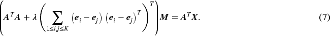
In this section, we discuss the optimization of the penalized K-Means problem defined in equation (6) and provide an algorithm to determine the optimal number of clusters for a given tuning parameter $\lambda$ . To obtain the optimized cluster centers, we differentiate equation (6) with respect to $\mathit{M}$ and equate to $0$ and obtain,

$$({\mathit{A}}^T\mathit{A}+\lambda {\left(\sum _{1\le i,j\le K}({\mathit{e}}_i-{\mathit{e}}_j){({\mathit{e}}_i-{\mathit{e}}_j)}^T\right)}^T)\mathit{M}={\mathit{A}}^T\mathit{X}.$$

(7)

More simplification of equation (7) is possible through some algebraic manipulation. Following Chi and Lange (2015), for $K=K^{*}$ we can obtain,

$$\sum _{1\le i,j\le K^{*}}({\mathit{e}}_i-{\mathit{e}}_j){({\mathit{e}}_i-{\mathit{e}}_j)}^T=K^{*}\mathit{I}-\mathbf{1}{\mathbf{1}}^T$$

(8)

where $\mathbf{1}$ is a $K^{*}$ length vector of 1 and $\mathit{I}$ is a $K^{*}\times K^{*}$ indicator matrix. Moreover, the matrix in the right-hand side of equation (8) is symmetric. Therefore, from equation (7) and (8), solution to the estimated cluster centers for a fixed number of cluster (in this case, $K^{*}$ ) are,

$$\hat{\mathit{M}}={({\mathit{A}}^T\mathit{A}+\lambda (K^{*}\mathit{I}-\mathbf{1}{\mathbf{1}}^T))}^{-1}{\mathit{A}}^T\mathit{X}.$$

(9)

We have also derived an unbiased estimator of the degrees of freedom for the fitted model (see Appendix 4), which can be used to compute any goodness-of-fit statistic. Note that for a fixed number of clusters, the optimized cluster centers can be estimated directly. However, the problem at hand involves simultaneously estimation of both the number of clusters and the cluster centers. To address this, we propose Algorithm ??, which performs a grid search to jointly optimize the cluster number $K$ and the estimated cluster centers $\hat{\mathit{M}}$ . Using Algorithm ??, one can obtain appropriate cluster assignments for all data points. Note that the algorithm operates for a fixed value of the tuning parameter $\lambda$ . Since the optimization problem includes a penalty on the cluster centers, the value of $\lambda$ influences both the number of clusters and the resulting cluster centers. As with any regularization-based approach, selecting an appropriate tuning parameter is crucial in penalized K-Means. It significantly impacts not only the quality of the resulting clustering but also the convergence behavior of the algorithm. In the following section, we describe the criteria used for selecting the tuning parameter.

5. Selection of Tuning Parameter

The estimated number of clusters and the corresponding cluster assignments in penalized K-Means clustering depend on the value of the non-negative tuning parameter $\lambda$ . Smaller values of $\lambda$ tend to yield more clusters, while larger values encourage fewer clusters, thereby controlling the trade-off between model fit and model complexity. To appropriately tune $\lambda$ , we adopt a clustering stability-based approach, as proposed in Fang and Wang (2012), Sun et al. (2012) and Wang et al. (2016) for the penalized K-Means framework. A cluster assignment is considered stable if perturbations in the data (e.g., through subsampling) result in minimal changes to the clustering outcome. The stability measure utilized in Sun et al. (2012) and Wang et al. (2016), tunes both the number of clusters $K$ and the Lagrangian tuning parameter $\lambda$ . However, since the penalized K-Means algorithm provides the optimal number of clusters $K$ for fixed $\lambda$ , we adapt the stability-based selection procedure to optimize only the tuning parameter $\lambda$ . The modified stability selection mechanism for identifying the most appropriate value of $\lambda$ along with the corresponding $K$ for a given dataset is described next.

Suppose that we have optimized the Algorithm 1 on the set of $\lambda$ values, ${\lambda }^{*}=\{{\lambda }_1,{\lambda }_2,\dots ,{\lambda }_l\}$ to obtain corresponding cluster assignments ${\mathbf{\Phi }}_{{\lambda }_1}(\cdot ),{\mathbf{\Phi }}_{{\lambda }_2}(\cdot ),\dots ,{\mathbf{\Phi }}_{{\lambda }_l}(\cdot )$ with estimated number of clusters $K_{{\lambda }_1},K_{{\lambda }_2},\dots ,K_{{\lambda }_l}$ respectively. If available, then let us denote the original assignments or true labels as ${\mathbf{\Phi }}^{Truth}(\cdot )$ . Draw $B$ many bootstrap samples without replacement ${\mathit{X}}^{*1},{\mathit{X}}^{*2},\dots ,{\mathit{X}}^{*B}$ , each with observation $n^{*}<N$ from the original data $\mathit{X}$ . Remember for fixed ${\lambda }_i$ we have optimized assignment ${\mathbf{\Phi }}_{{\lambda }_i}(\cdot )$ with $K_{{\lambda }_i}$ clusters for $i=1,2,\dots ,l$ . Therefore for each ${\lambda }_i$ we optimize Algorithm 1 on each bootstrap sample ${\mathit{X}}^{*b}$ such that, we obtain exactly $K_{{\lambda }_i}$ clusters with assignments ${\mathbf{\Phi }}_{{\lambda }_i}^{*b}(\cdot )$ where $b=1,2,\dots ,B$ denoting the $b^{th}$ bootstrap sample. We define two types of stability measure,

If the true labels ${\mathbf{\Phi }}^{Truth}(\cdot )$ are available then we define the true stability as the average agreement between the true labels and the predicted assignments in the bootstrap samples,

$${\hat{\mathit{S}}}_{{\lambda }_i}^{Truth}={\displaystyle \frac{1}{B}}\underset{b=1}{\sum ^B}\mathbf{\Gamma }({\mathbf{\Phi }}^{Truth}({\mathit{X}}^{*b}),{\mathbf{\Phi }}_{{\lambda }_i}^{*b}({\mathit{X}}^{*b}))$$

(10)

where $\mathbf{\Gamma }(\cdot ,\cdot )$ is some concordance measure between the cluster assignments.

For data without any class or label information, the predicted stability measure is defined as the average concordance between the predicted cluster assignment ${\mathbf{\Phi }}_{{\lambda }_i}(\cdot )$ and the corresponding cluster assignments on the bootstrap samples ${\mathbf{\Phi }}_{{\lambda }_i}^{*b}(\cdot )$ , evaluated using a chosen measure of association $\mathbf{\Gamma }$ ,

$${\hat{\mathit{S}}}_{{\lambda }_i}^{Predicted}={\displaystyle \frac{1}{B}}\underset{b=1}{\sum ^B}\mathbf{\Gamma }({\mathbf{\Phi }}_{{\lambda }_i}({\mathit{X}}^{*b}),{\mathbf{\Phi }}_{{\lambda }_i}^{*b}({\mathit{X}}^{*b})).$$

(11)

A common choice for the association/concordance measure in is the Rand Index (Rand, 1971). The stability index $(\hat{\mathit{S}})$ defined in Sun et al. (2012) can be written in terms of Rand Index $(\mathcal{R})$ as, $\hat{\mathit{S}}=1-\mathcal{R}({\mathcal{C}}_1,{\mathcal{C}}_2)$ , with two cluster assignments ${\mathcal{C}}_1$ and ${\mathcal{C}}_2$ . Several drawbacks of the Rand Index as a similarity measure have been identified. Morey and Agresti (1984) and Fowlkes and Mallows (1983) showed the high dependence of the Rand Index on the number of clusters and it converges to 1 with an increase of cluster number, which we also have observed. Moreover Rand Index also suffers from association by random chance. Thus it yields higher values for certain random clustering that does not coincide with the true labeling of the data. Nonetheless, the concept of concordance captured by the Rand Index remains valuable, particularly for detecting the number of clusters. To address these limitations, we adopt the Adjusted Rand Index (ARI; see Halkidi et al., 2002; Hubert & Arabie, 1985) as the measure of association $\mathbf{\Gamma }$ . ARI is a standardized version of the Rand Index that corrects for both random chance and the inflation caused by higher numbers of clusters. ARI index value is equal or close to 1 only for the homogeneous assignments on bootstrap samples and true/predicted assignments and close to 0 for a random partition. The best value of tuning parameter $\lambda$ and corresponding cluster number is chosen as

$$\hat{\lambda }=\underset{{\lambda }_i\in {\lambda }^{*}}{argmax}{\hat{\mathit{S}}}_{{\lambda }_i}^{Predicted}.$$

If multiple values of $\lambda$ produce the optimal ${\hat{\mathit{S}}}^{Predicted}$ , then we choose the best $\lambda$ and $K$ in the following manner. Let ${\hat{\lambda }}^1,{\hat{\lambda }}^2,\dots ,{\hat{\lambda }}^r$ are the $\lambda$ values corresponding to optimal ${\hat{\mathit{S}}}^{Predicted}$ with cluster numbers $K^1,K^2,\dots ,K^r$ respectively. Then we have the optimal cluster number, $\hat{K}=mode\{K^1,K^2,\dots ,K^r\}$ and estimate of the tuning parameter

$$\hat{\lambda }=\underset{\hat{\lambda }}{min}\{{\hat{\lambda }}^i:|{\mathcal{C}}_{{\hat{\lambda }}^i}|=\hat{K};\mathrm{\forall }i\in (1,2,\dots ,r)\}.$$

6. Simulation Study

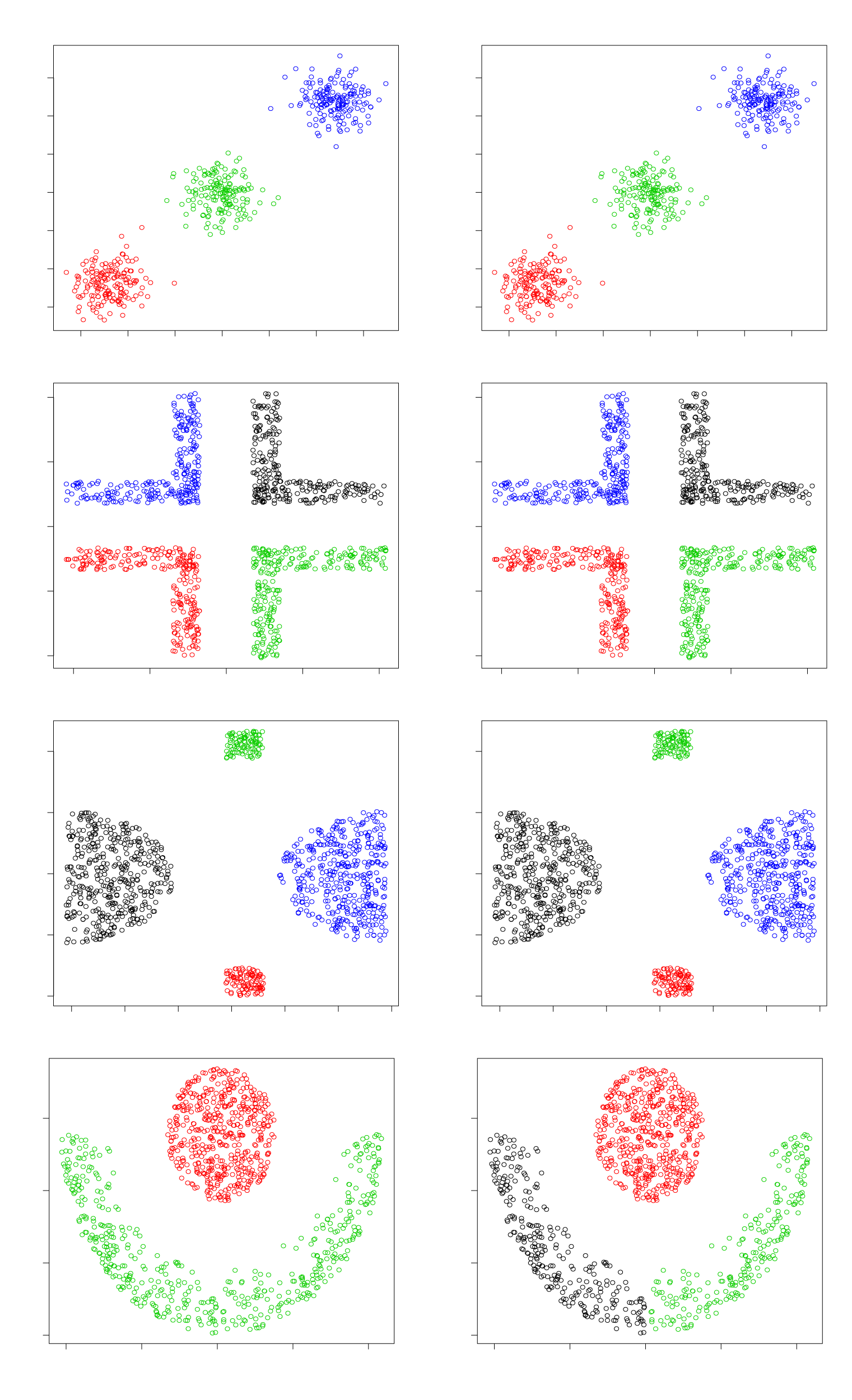
The performance of the augmented K-Means clustering algorithm is first evaluated on several simulated benchmark datasets. Four separate benchmark datasets are selected for testing purposes, as detailed below:

Three Gaussian clusters (Tan & Witten, 2015) are generated with $n=500$ and $p=2$ . The $n\times p$ data matrix $\mathit{X}$ is generated from $\mathcal{M}\mathcal{V}\mathcal{N}({\mathit{\mu }}_k,1.5*\mathit{I})$ . The mean vectors ${\mathit{\mu }}_k$ are assigned as ${\mathit{\mu }}_1=-3\cdot {\mathbf{1}}_{\mathit{p}},{\mathit{\mu }}_2=0\cdot {\mathbf{1}}_{\mathit{p}},\text{and}{\mathit{\mu }}_3=3\cdot {\mathbf{1}}_{\mathit{p}}$ respectively for three clusters. The points are equally distributed among the three clusters such that each point corresponds to a unique cluster.

Second simulated setup is the four corners data from Karami and Johansson (2014). A total number of $n=1000$ points are chosen in such a way that each belongs to a specific corner.

The outlier data (Karami & Johansson, 2014) with $n=1000$ points are also considered in the simulation study. Data consists of two large half-circular regions and two smaller outlier regions.

The final benchmark dataset used in the simulation study is the crescent full moon dataset (Karami & Johansson, 2014), which consists of 500 data points arranged in a circular region and another 500 points forming a half-moon shape.

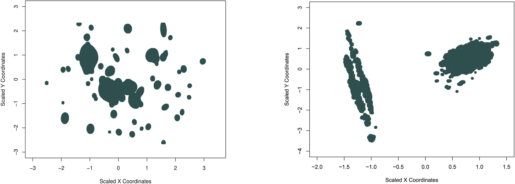
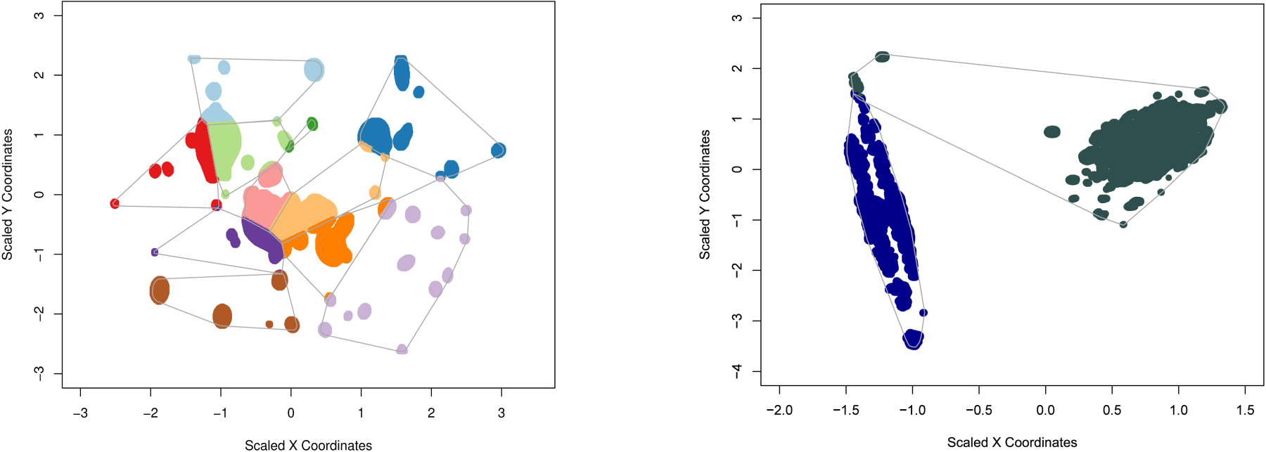
On each of the datasets, we have optimized the penalized K-Means algorithm on a grid of $\lambda$ values. For each $\lambda$ , the algorithm is optimized to obtain the best cluster number $K$ . The optimum $\lambda$ and corresponding cluster number $K$ is chosen via the stability measure mentioned above. Figure 1 illustrates the original cluster assignments alongside the best predicted cluster assignments for the four simulated examples. The first row of the panel corresponds to the Gaussian clusters, the second row to the corners data, the third row to the outlier data, and the fourth row to the crescent full moon dataset. The proposed augmented K-Means clustering method accurately detects both the number and the locations of clusters in all cases, with the exception of the crescent full moon data. In that case, the method partitions the crescent moon into two separate clusters. This result is not unexpected, as a key assumption in augmented K-Means is that the cluster center should lie within the convex hull of the points in that cluster. This assumption is violated in non-convex structures like the crescent moon. Thus, for the non-convex shape of the crescent moon, the best possible clustering while adhering to the convex center construction constraint is shown in the last plot of the right panel in Figure 1. It is worth noting that with an appropriate choice of a loss function that accounts for non-convex cluster structures, it is possible to modify the optimization problem presented in equation (3). However, such a modification would require further methodological developments to effectively solve the resulting optimization problem, which is beyond the scope of the current paper.

Figure 1.

True Cluster Assignment (Left Panel) vs. Predicted Cluster Assignments (Right Panel). The X and Y Axes Represent the Two Dimensions Used for Data Generation and Clustering.

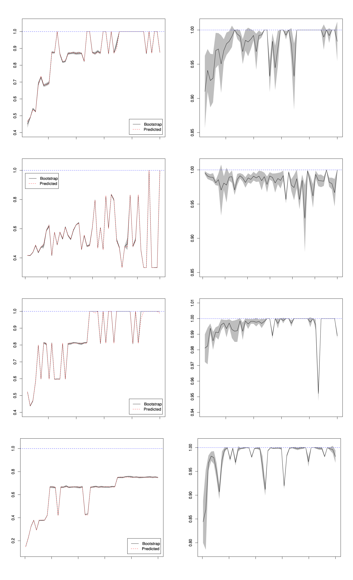
The next panel of plots in Figure 2 demonstrates the performance of the augmented K-Means clustering algorithm for different values of tuning parameter $\lambda$ . In all the plots, we kept the values of $\lambda$ along the x-axis, and the versions of the ARI along the y-axis. The plots are arranged in the same order of benchmark datasets as Figure 1. The plots on the left panel show the predicted ARI (in red dashed line) and the bootstrap version of ARI (solid black line) calculated with respect to the true response values. The close resemblance between the two curves is clearly visible, showing the stability of the proposed measure for identifying the best tuning parameter. The preferred choice of clusters is the clusters corresponding to the chosen tuning parameter. We see several ties of $\lambda$ values (yielding ARI as $1$ ) in the first three plots in the left panel of Figure 2. In those cases, the best choice of $\lambda$ is determined as mentioned in Section 5, which is the minimum value yielding one. This is not true for the fourth dataset of crescent full moon though, where ARI never reached unity as the best clustering detected by our algorithm is not an exact match with the truth. The plots in the right panel show the predicted ARI (solid line) along with its confidence bound with respect to the predicted clusters for each value of $\lambda$ . An almost identical pattern as the true ARI (in the left panel) can be noticed for the predicted ARI. A similar idea is implemented to break the ties and choose the best values of tuning parameter $\lambda$ and corresponding optimum cluster assignments. The plots in the right panel of Figure 1 showing the cluster assignments correspond to the optimum choice of $\lambda$ chosen through the predicted ARI. Note that for real data though, we do not observe any response/outcome, calculating the ARI is therefore infeasible and we resort to the predicted ARI, to optimize the tuning parameter for the proposed augmented K-Means algorithm.

Figure 2.

True and Bootstrap Version of Adjusted Rand Index (Left Panel) and the Predicted Adjusted Rand Index (Right Panel) in the Y-axis and for Different Values of $\lambda$ Along the X-axis.

7. Application on Globular Clusters Detection

Clustering is a very common problem with many application domains and as such our algorithm proposed in this article is fairly general. We choose the field of astronomy as the detection of star clusters and galaxies is a very important and challenging problem with unknown cluster numbers. This field often produces a single image large enough so that it cannot be loaded in the memory of a personal computer resulting in truly Big Data ( $N\uparrow$ ) (Estévez, 2016; Loredo et al., 2009; Mickaelian et al., 2016). For our purpose, we considered publicly available NASA Hubble telescope images. These galaxy(s) or star clusters are globular in nature and thus can be categorized into convex clusters via a clustering mechanism based on centers. We intend to test the performance of the augmented K-Means algorithm to detect the number and location of globular clusters present in an image of galaxies and star clusters. Two separate images with distinct characteristics are considered for this work, both downloaded from NASA (2015) and NASA (2017) respectively. Figure 3 shows the original images, with lots of possible galaxy and star clusters from Hubble deep space image (left) and two sister galaxy images (right). Some pre-processing mechanism was implemented on the images to remove the noises before running the clustering mechanism. The image pre-processing steps are as follows,

First we converted the color image to gray-scale. This is done as otherwise color temperature at each pixel poses as a separate dimension.

The images are then processed, in order to remove the background noises and detect pixel values (location and intensities).

Pixels are segmented and those with intensities more than the ${95}^{th}$ percentile are considered for the analysis, rest ignored.

Image data are arranged to have a final data frame with pixel locations and corresponding gray-scale intensities.

Note that, other pixel intensity percentiles can be considered, but we stick with ${95}^{th}$ as it provided the best noise reduction of the images. We utilized the $\mathrm{R}$ (R Core Team, 2015) package “imager” (Simon, 2017) for the image pre-processing. After pre-processing, the denoised images are shown in Figure 4, where the colored space is the pixels considered for the clustering analysis. Before denoising the Hubble deep space image, we had around $304704$ pixels and their corresponding intensity values, which were reduced to $30690$ after the pre-processing. Similarly, for two sister galaxy images, we had $12517416$ pixels which after noise reduction was scaled down to $657694$ pixels for the final analysis. Analogous to the simulation study we optimized the augmented K-Means algorithm for each tuning parameter value $\lambda$ to obtain the predicted clusters. We have chosen a fine grid of $\lambda$ values ranging from 0 to 10, for our analysis. The number of possible cluster numbers are considered as 100 and 10 respectively for the two data sets. The model optimization is computationally expensive and requires large memory for both data and storage. Thus, is not possible to run on normal desktops or laptops even with parallel frameworks. We utilized the grid computing nodes of Wayne State University to run the optimization algorithm and final prediction.

Figure 3.

Lots of Galaxies Image (Left) and Two Galaxies Image (Right).

Figure 4.

Image After Preprocessing for Galaxy Cluster Data (Left Panel) and Two Sister Cluster (Right Panel).

Figure 5.

Predicted Adjusted Rand Index ( $1^{st}$ Row) and the Estimated Clusters ( $2^{nd}$ Row) for Galaxy Cluster Data (Left Panel) and Two Sister Cluster (Right Panel) with the Predicted Tuning Parameter $\lambda$ (Red Dashed Line).

Figure 6.

Predicted Clusters and Corresponding Assignments for (Left) Galaxy Cluster Data with 11 Clusters and (Right) Two Sister Galaxy with 2 Clusters. The Line Within Each Figure Indicates the Outer Shape of Each Cluster.

The next panel of plots in Figure 4 shows the images after the pre-processing and thresholding. In Figure 5 we have plotted the predicted ARI values and the estimated clusters for both datasets. An optimum value of the tuning parameter $\lambda$ is presented as the red dashed line. For all the plots, we kept the values of $\lambda$ along the x-axis the predicted ARI (for 1st row of the panel), and the predicted cluster number (for 2nd row of the panel) along the y-axis. It can be observed that the optimum cluster number for the Hubble deep space image is 11 whereas 2 clusters are observed for two sister galaxies. Finally in Figure 6, we have shown the best cluster assignments among different galaxies. A point to note is that the images (as drawn) are the 2D representation of the original 3D space (consisting of pixel x-coordinate, pixel y-coordinate, and intensities). Moreover, the optimization of clusters is done in the transformed space rather than the original space. If we revert to the original space, the assignments are better, but the pictorial demonstration is not optimum.

8. Conclusion and Future Direction

Despite its limitations and computational challenges when applied to large, heterogeneous datasets, K-means clustering remains one of the oldest and most widely used clustering algorithms. However, traditional K-means is prone to overfitting and often converges to local minima. In this work, we revisit the method with the aim of mathematically characterizing some of its limitations. To address these issues, we propose a penalized version of K-means clustering that enables automated selection of the number of clusters, followed by cluster assignment. Our approach relies on the appropriate selection of a tuning parameter, which plays a crucial role in balancing model complexity and fit. There are several directions in which this work can be extended, and we outline a few of these as potential avenues for future research.

In typical cluster analysis, all available features are often assumed to be useful. However, in practice, not all features are equally informative—or even relevant—for the clustering task. This motivates the incorporation of feature selection prior to clustering, as discussed in Raftery and Dean (2006) and Witten and Tibshirani (2010). Effective feature selection can significantly influence the resulting cluster structure, including the estimated number of clusters. However, stepwise procedures—where features are selected first and the number of clusters $K$ is determined afterward—may be suboptimal, as errors introduced in the earlier step cannot be corrected later. Consequently, the simultaneous selection of relevant features and the optimal number of clusters $K$ remains a challenging and largely unresolved problem.

As noted throughout the paper, our method is based on K-means and is therefore best suited for convex clusters, where the notion of a cluster center is naturally meaningful. However, real-world data often exhibit non-convex or even irregularly shaped clusters, where this concept becomes less interpretable. In such cases, alternative formulations of the clustering objective are required. Pan et al. (2013) investigated clustering methods involving non-convex penalties, and more recently, Wu et al. (2016) proposed computationally efficient adaptations of such approaches. Nevertheless, both studies continued to rely on convex loss or distance functions. The estimation of the number of clusters under non-convex loss functions remains a challenging and largely unresolved problem.

Centroid-based clustering under non-convex metrics represents a compelling area for future research, posing both theoretical and computational challenges. Another promising direction involves clustering data that do not follow a continuous distribution, which demands the development of novel distance metrics. Identifying the number of clusters in such settings presents an intriguing and worthwhile avenue for further investigation.

Supplemental Material

sj-pdf-1-mod-10.1177_15741699251377692 - Supplemental material for Penalized K-Means Clustering: Another Look at Its Statistical Properties

Supplemental material, sj-pdf-1-mod-10.1177_15741699251377692 for Penalized K-Means Clustering: Another Look at Its Statistical Properties by Prithish Banerjee, Shreyo Ghosh and Samiran Ghosh in Model Assisted Statistics and Applications