
Abstract
In the contemporary global landscape, there has been a growing uncertainty due to continuous shocks with significant implications on investment and portfolio management. This paper investigates how return spillovers and dependencies between traditional and modern financial assets evolve under varying market conditions, with a focus on the COVID-19 crisis period. Using a quantile vector autoregression (QVAR) model combined with network analysis, we analyse daily asset returns from 02 January 2018 to 30 June 2023 to capture asymmetric and state-dependent connectedness. The study reveals that asset interdependencies intensify during periods of market stress, particularly at extreme quantiles. Green bonds, gold, and AI-related assets exhibit safe-haven characteristics under these conditions. The findings underscore the dynamic nature of market connectedness and provide important insights for portfolio diversification strategies, especially for risk-averse investors navigating turbulent markets.
Introduction
In recent times, the global financial landscape has undergone rapid transformations, primarily driven by the swiftly evolving technological environment and the subsequent emergence of technology-centric asset markets (Arslanian & Fischer, 2019). Amidst these changes, a topic of considerable academic and practical interest revolves around the extent and mechanisms of integration between markets characterized by diverse attributes and purposes. Portfolio management and investment strategies have been perennial areas of concern, and both scholars and practitioners have dedicated their efforts to devising methods that facilitate effective portfolio construction, ensuring adequate risk diversification. The increasing globalization of financial markets has given rise to ever-growing interconnections between the returns and volatility of various investment assets. Consequently, during periods of market turmoil, the options for diversification become scarcer, compelling investors to seek out new investment avenues that exhibit either no correlation or negative correlation with major asset classes. More recently, investors have begun to explore the investment prospects presented by the Fourth Industrial Revolution (4IR) when constructing portfolios. The advancements in fields like Artificial Intelligence (AI), Financial Technology (FinTech), and developments in blockchain systems within the context of this revolution are swiftly ushering in a new era of global economic activity.
The COVID-19 pandemic induced-crisis received extensive coverage and has been compared to the 2008 Global Financial Crisis. This crisis presented both challenges and opportunities in various asset markets. It significantly increased risk and volatility across financial, traditional, and modern asset markets, affecting risk management efforts. For instance, Commodity markets experienced heightened volatility due to the pandemic (Bakas & Triantafyllou, 2020). However, the pandemic also brought about opportunities. It accelerated trends such as increased online shopping and remote work, benefiting e-commerce and technology companies. Demand for reliable internet connectivity, contactless payments, and digital wallets grew. This led to investments in areas like e-commerce, cloud computing, cybersecurity, FinTech, Cryptocurrencies (like Bitcoin and Ethereum), and 5G infrastructure among telecommunications companies.
Understanding the relationships between traditional and modern assets is crucial for investors and market participants. Strong correlations among these assets may lead to hedging strategies, where investors go long on one type of asset and short on the other to manage risk. Conversely, weak correlations suggest diversification opportunities. In times of market turbulence, assets with low and consistent correlations can act as safe havens, providing stability. Traders operating in both markets need to be aware that trends affecting traditional assets can influence demand for modern assets and even affect hedging strategies. Therefore, assessing interconnections between these asset markets is essential for effective portfolio management and trading strategies.
The rise in technology-related assets in the investment landscape includes Cryptocurrencies, FinTech, Green bonds, and AI. These assets have gained prominence since the 2008 Global Financial Crisis and are increasingly influencing traditional markets. Few existing literatures has focused on the linkages between these modern assets and traditional ones, with an emphasis on Cryptocurrencies (Abakah et al., 2020; Shahzad et al., 2019; Wu et al., 2021). Studies have revealed strong return connectedness, especially during extreme market conditions, and the potential for modern assets to promote sustainability in the financial industry. This paper highlights the growing significance of twenty-first-century assets in investment portfolios and their impact on global financial markets.
The mentioned prior studies contextualise on how technology-related assets are globally integrated with global stock markets and Green bonds. However, the current empirical knowledge in this area focuses solely on the connections between Cryptocurrencies and traditional assets. This paper addresses a gap in the existing research by examining how various modern technology-related assets interact with traditional markets. It investigates the convergence and spillover effects of returns across these markets in the context of the 4IR to improve portfolio diversification strategies. The study is motivated by the interconnectedness of financial markets, economic cycles, and the impact of technology-related asset price fluctuations on broader financial markets (Tiwari et al., 2023). It aims to evaluate the predictability and correlations among traditional and modern markets, particularly during extreme events, to enhance investment strategies and diversification.
While technology plays a pivotal role in shaping contemporary asset markets, the causal relationships and durations involved can vary, contingent on the specific dynamics within a given market and the necessity of these assets within portfolio construction. Recognizing the existing parallel conclusions in the literature regarding the intricate connections between diverse traditional and modern assets, the paper aims to answer the questions: (i) Are traditional-modern asset relationships time-varying, crisis-sensitive and does the relationship entails complementary or substitution implications pre-, during and post-crisis; (ii) how can investors diversify portfolios among traditional and modern assets? and (iii) Is there a divergent transmission mechanisms and dependence between the traditional-modern asset classes under examination during heterogenous market states?
This paper offers a contextualized and empirically rich examination of return interdependencies across a diverse set of traditional and modern technology-driven assets, including FinTech, AI, Green Bonds, and Cryptocurrencies. Previous studies have primarily focused on bilateral relationships, often between traditional financial assets and Cryptocurrencies. This study expands the scope by incorporating a broader asset mix and analyzing their dynamic connectedness across different market regimes surrounding the COVID-19 pandemic. The novelty of this work lies not in methodological innovation per se, but in the strategic integration of established techniques namely Quantile VAR and tail-risk measures (VaR, CVaR, and Expected Shortfall) to capture asymmetric spillovers and tail-dependent behavior across quantiles (τ = 0.1, 0.5, 0.9). This quantile-based approach enables a more nuanced understanding of systemic risk and asset behavior under extreme market conditions, which is particularly relevant for crisis-aware portfolio construction.
Importantly, the study distinguishes between diversification and hedging, clarifying the roles of assets as either shock absorbers or transmitters across different quantiles and time periods. While the analysis is limited to in-sample estimation and bivariate portfolio optimization, it provides a foundation for future research to incorporate multivariate frameworks and out-of-sample validation. By situating its contribution within the broader literature on financial connectedness and tail risk, this paper adds value through its empirical scope, quantile-specific insights, and relevance to both conventional and risk-sensitive investment strategies.
The rest of the paper is structured as follows: existing literature related to the paper is outlined in section 2. Empirical approaches and methodological framework used for this paper are outlined in section 3 while relevant data with its description, associated statistical properties, empirical results and discussions are presented in section 4. Lastly, the paper ends with concluding remarks and policy recommendations provided in section 5.
Literature Review
Conceptual Framework
Spillover effects in the context of this paper describes the transmission mechanism of shocks (negative and positive) from one asset to the other measured by extend to which one asset impacts the volatility of another asset. As per the theory of the Heterogeneous Market Hypothesis, participants in the market possess diverse goals and investment timeframes. They respond to information at varying points in time, leading to traditional and modern asset price series displaying characteristics like non-linearity, non-stationarity, and long-term memory, as outlined by Müller et al. (1993). The existence of non-linearity makes the application of conventional linear models unsuitable. Therefore, to gain a more comprehensive insight into their interconnection, it becomes crucial to employ analyses that consider the evolving nature of their relationships and the distributional dependencies that arise over time. Modern portfolio theory implies that gaining insights into the transmission of effects among financial markets provides valuable information for efficient risk reduction and diversification tactics. Furthermore, existing literature widely acknowledges that the transfer of influences within financial markets exhibits asymmetry, wherein positive and negative news propagate at varying rates (Markowitz, 1952).
Standard deviation, a common measure of risk, has limitations when dealing with non-normal return distributions, which has been recognized by various researchers (Markowitz, 1959; Ang et al., 2006). This limitation is especially evident in behavioural finance, where investors may have asymmetric attitudes toward gains and losses. To address this issue, an improved metric called semi-standard deviation was proposed by Rom and Ferguson in 1993. This metric accounts for the asymmetric behaviour of investors by distinguishing between extreme positive and negative volatilities. This concept of Post-Modern Portfolio Theory builds upon these ideas and aims to provide investors with better decision-making tools, considering the non-normality of return distributions. It offers flexibility to asset managers in their decision-making processes without necessarily resorting to alternative investments. Post-MPT also assists investors in pricing risky assets and optimizing their portfolios through diversification.
From a theoretical perspective, various pathways, and elements, as outlined in prior studies on intermarket dynamics, could contribute to establishing a link between the conventional stock market and the modern/technology-driven stock markets. The first of these pathways is the correlated-information channel, as described by Kodres and Pritsker (2002), where connections arise through the price discovery process. The second pathway is the risk premium channel, in which a disruption in one market can negatively impact the inclination of market participants to bear risks in any market, as proposed by Acharya and Pedersen (2005). Both channels are relevant to the case of traditional-modern assets nexus.
Empirical Review
This paper is part of a growing body of research that explores the connectedness between various financial markets and asset classes, especially in the context of diversification strategies involving technology-oriented assets. It draws from four main branches of literature, covering interdependencies among traditional and modern assets, the connection between different types of assets, transmission across assets using various techniques, and changes in market interdependencies during crisis periods. The paper aims to bridge these areas of literature by examining spillovers between traditional and modern asset returns using quantile connectedness approaches, with a focus on the recent COVID-19 crisis.
Various studies have explored the connections between modern assets, like Cryptocurrencies, and traditional assets, focusing on their role in portfolio diversification and as potential safe havens during market events. However, the results from these studies have been inconsistent and inconclusive. For instance, some research, such as Mensi et al. (2023), examined the return spillovers between Cryptocurrencies and Gold, while Liu et al. (2020) investigated spillover effects between Cryptocurrencies and FinTech assets. These studies found bidirectional relationships with significant spillover effects in both directions. On the other hand, Le et al. (2020) explored volatility spillovers between FinTech, Gold, Oil, Green bonds, and Bitcoin. They revealed that FinTech assets contributed significantly to volatility shocks, and traditional and emerging assets acted as hedges against FinTech assets. Furthermore, Le et al. (2021) analysed spillovers among returns from FinTech, Green bonds, and Cryptocurrencies. They found high total connectedness among modern and traditional assets, indicating a high likelihood of concurrent losses during extreme market conditions. To address these inconsistencies, this paper employs quantile tail techniques to analyse the nature of relationships, optimal portfolio construction, and spillover patterns among various modern and traditional assets. The aim is to optimize portfolio returns, particularly during times of crisis. It's important to note that these existing studies conducted time-varying analyses and confirmed that the connectedness among traditional and modern assets increased due to idiosyncratic shocks across different market conditions.
Another strand of studies explored the relationships among modern and emerging asset classes, emphasizing their role in diversifying portfolios and responding to different market conditions.
Corbet et al. (2018) investigated the spillover effects involving Cryptocurrencies and other assets like stock indices, Commodities, and currencies. Their findings highlighted that Cryptocurrencies were influencing stock indices, indicating their integration into the global financial system. Previous studies by Bouri et al. (2017) and Demir et al. (2018) had also recognized the hedging potential of Cryptocurrencies, particularly during extreme market conditions. Ballis et al. (2025) analysed how asset spillovers changed during times of crisis. They found that Cryptocurrency markets tended to act as a hedge against uncertainty, responding positively to uncertainty at both higher quantiles and shorter-term fluctuations.
Symitsi & Chalvatzis (2018) explored asymmetric nonlinear relationships between aggregated Cryptocurrency prices, Commodity prices, and Gold prices. The study identified return spillovers from traditional stock indices to Cryptocurrency, highlighting the benefits of including Cryptocurrency in a portfolio due to its low correlation with traditional assets.
Jin et al. (2019) investigated the relationships among Cryptocurrency, Gold, and crude Oil markets. They noted that the Gold market played a dominant role in absorbing new information, especially compared to Crude Oil and Cryptocurrency markets. Uroma et al. (2020) studied time-varying dependence and directional predictability from Bitcoin to developed equities, crude Oil, and Gold. Their findings showed strong evidence of time-varying volatility levels among these assets. Notably, while these studies focused on exploring the relationships among these assets, they often concentrated on Cryptocurrencies and did not examine a diverse range of modern asset classes.
Numerous studies have explored the transmission of shocks across financial assets using a variety of econometric and statistical techniques. However, many of these methods rest on restrictive assumptions that limit their effectiveness in capturing the complex, nonlinear, and asymmetric dynamics often observed in financial markets. For instance, models such as conditional correlation, ARDL, and multivariate GARCH typically assume linear relationships, symmetric responses, and often normality of errors, which may not hold during periods of market stress or extreme events (Adebola et al., 2019; Ji et al., 2019; Shahzad et al., 2019). Wavelet analysis, while useful for time-frequency decomposition, lacks a probabilistic framework and is sensitive to methodological choices such as wavelet type and boundary conditions. Similarly, TVP-VAR models, as used by Kumar et al. (2023), allow for time-varying dynamics but still rely on mean-based relationships and may not adequately capture tail dependencies or distributional asymmetries. Granger causality and copula-based approaches, though capable of identifying directional and nonlinear dependencies, are often limited by their reliance on specific distributional assumptions and are difficult to scale in high-dimensional settings. CoVaR and non-parametric causality techniques, such as those employed by Abakah et al. (2022), provide insights into systemic risk and interdependence but are typically pairwise and do not account for the broader network structure of interconnected markets. In contrast, the Quantile VAR (QVAR) framework adopted in this study offers a more flexible and robust approach by modelling the entire conditional distribution of asset returns. It captures asymmetric spillovers and tail-specific connectedness, making it particularly suitable for analysing systemic risk and shock transmission under varying market conditions. By allowing for quantile-specific impulse responses and integrating seamlessly with network analysis, QVAR overcomes many of the limitations inherent in traditional models and provides a richer understanding of financial interconnectedness (Ando et al., 2022; Diebold and Yilmaz, 2012).
Recent financial and economic crises, including the COVID-19 pandemic, have led to a focus on understanding changes in market interdependencies and return transmission during stress periods (Mensi et al., 2016). Studies have explored how these crises affected the relationships between diverse asset classes, influencing asset allocation and hedging strategies. For example, research has revealed changes in interdependence among financial markets, particularly during crises (Demiralay et al., 2021; Shaik et al., 2023). Some studies have shown positive returns in modern technology-driven sectors during the COVID-19 crisis (Abakah et al., 2022; Conlon and McGee, 2020; Mazur et al., 2020), while others have examined the transmission of financial contagion and increased correlations during the pandemic (Akhtaruzzaman et al., 2020; Kumar et al. 2023; Le et al., 2021). However, none of these studies have conducted a comprehensive analysis that spans pre-crisis, during-crisis, and post-crisis phases, covers various modern asset classes, and uses different risk measures to compare portfolio compositions across these periods.
Contextualizing the above review, prior research has highlighted that the interconnectedness between traditional and modern assets is complex and subject to change. It depends on factors such as the time period and the types of assets involved in each market. The roles of traditional and modern assets as hedges, diversification tools, or safe havens vary significantly depending on market conditions. This underscores the importance of assessing these interdependencies for investment decision-making. Analysing the interconnectedness of traditional and modern assets, especially in the context of the COVID-19 pandemic, offers opportunities for optimizing portfolios during financial crises. During the pandemic, there might be increased linkages between these asset classes, and the nature of these relationships may differ depending on market conditions. Existing studies have used various approaches to explore these relationships, but few have investigated them using different tail-risk measures across various sub-sample distributions. Robust analysis should encompass a diverse range of modern and traditional asset classes to provide reliable insights into their relationships and diversification potential. Such analyses can guide investors and asset managers in optimizing portfolio allocations under different market conditions.
Methodology
Quantile Connectedness
In this paper, a quantile connectedness framework, as explained by Ando et al. (2022), is employed to gauge both the direction and magnitude of return interdependencies among traditional and modern assets across various quantiles. This approach assesses connectedness under heterogenous market conditions, utilizing a straightforward measure of volatility spillovers as originally established by Diebold and Yilmaz (2009, 2012).
Adoption of this technique offers distinct advantages including facilitating a more comprehensive grasp of the dynamics within transmission mechanisms, and enables the measurement of asymmetries in the transmission of volatility utilizing a methodology proposed by Baruník and Křehlík (2018). In contrast to the conventional mean-based connectedness measures derived from Diebold and Yilmaz (2012)'s framework of quantile-based measures of connectedness, this method considers a VAR system comprising m assets with the optimal lag order p determined using the Akaike Information Criteria (AIC). The VAR model at a particular


To derive the connectedness indices based on Diebold and Yilmaz (2012), the Equation (1) is transformed into an infinite moving average representation:

According to Pesaran and Shin (1998), the Generalized Forecast Error Variance Decomposition (GFEVD) quantifies how much each variable contributes to the forecast error of another variable at a specified quantile and forecast horizon (Diebold and Yilmaz, 2012):
Using the GFEVD, the paper calculates at each quantile four measures of connectedness. Firstly, the Total Connectedness Index (TCI) at

Secondly, the directional spillover index received (FROM) by asset i from all other assets j at

Thirdly, contrary to the above, directional spillover index transmitted (TO) by asset i to all other assets j at

Lastly, net spillover index (NSI) from one asset to all others at a specific quantile is calculated by subtracting the gross volatility shocks transmitted to that asset from those received from all other assets at that quantile:

If the value is positive (negative), it indicates that the asset is a net-transmitter (net-recipient) of shocks to other markets. This calculation is performed using a Quantile VAR model with a lag order of 1, selected based on the Bayesian Information criterion, and a forecast horizon of 10. The approach follows Lee et al. (2020) by estimating dynamic connectedness over a 200-day rolling window at each quantile.
In addition to quantile connectedness techniques, this paper employs tail-risk measures such as Value at Risk (VaR), Conditional Value at Risk (CVaR), and Expected Shortfall (ES) to optimize portfolios. Assuming “

VaR represents the maximum potential loss over a specified time horizon with a certain confidence level (Chai and Zhou, 2018). However, CVaR, which is more effective for continuous distributions and high volatility assets, is used to address the limitations of VaR. The decision to use tail-risk measures in portfolio optimization is based on the substantial return connectedness in the lower tail of both traditional and modern assets.
CVaR assesses the expected losses in the tail of the return distribution, but it goes beyond VaR by considering the entire spectrum of price movements (Rockafellar and Uryasev, 2000). Unlike VaR, which marks a specific point, CVaR looks at the continuous price dynamics of assets. To calculate the CVaR at a confidence level
Artzner et al. (1999) also addressed the shortcomings of VaR by introducing ES as another alternative risk measure which effectively addresses the issues and is defined as follows:

From observation, the two measures of risk are closely related to each other.
To rigorously assess the financial implications of this study, a historical back testing framework that contrasts traditional portfolio construction methods with advanced strategies informed by asset interconnectedness is implemented. Drawing on the methodology of Broadstock et al. (2022), an application of multivariate optimization techniques to evaluate the effectiveness of risk mitigation mechanisms is adopted within dynamic market environments.
Among the optimization strategies considered, the Minimum Variance Portfolio (MVP) aims to minimize portfolio volatility by optimizing asset weights based on individual variances and covariances. This approach aligns with the principles of Modern Portfolio Theory (Markowitz, 1959), emphasizing capital preservation and appealing to investors with low risk tolerance. The MVP is mathematically formulated as:

In contrast, the Minimum Correlation Portfolio (MCP) seeks to enhance diversification by minimizing the average pairwise correlation among assets, rather than focusing solely on volatility. This strategy aims to reduce systemic co-movement, thereby stabilizing portfolio performance during market turbulence. However, its emphasis on low correlation may inadvertently exclude high-return assets that exhibit strong interdependence, potentially compromising return optimization.
Christoffersen, et al. (2014) introduced a portfolio construction methodology that leverages conditional correlations in place of traditional covariance measures. Conditional correlations are derived through the following matrix definition as follows:

Subsequently, the minimum correlation portfolio (MCP) asset weights are determined as follows:
A third approach, the Minimum Connectedness Portfolio (MCoP), integrates network theory to address systemic risk by minimizing the interconnectedness of assets within a financial network. This method captures spillover effects and contagion dynamics, offering a more holistic view of risk beyond traditional metrics. MCoP seeks to reduce systemic risk exposure by constructing a portfolio with minimized asset interdependence. In contrast to traditional approaches relying on variance or correlation, the MCoP leverages pairwise connectedness indices (Broadstock et al., 2022). This strategy emphasizes the selection of assets exhibiting weak mutual influence within the broader portfolio context, thereby enhancing robustness against systemic shocks. The constituent asset weights are calculated as follows:

Data and Variables Description
To explore the distributional and quantile connectedness across traditional and modern assets, the study collected secondary daily price data from DataStream covering all the global aggregate traditional and modern assets categories presented in Table 1 from 02/01/2018 to 30/01/2023 to consider periods pre-COVID-19 crisis (02/01/2018—28/02/2020), during the COVID-19 crisis (02/03/2020–31/03/2021) and post-crisis (01/04/2021–30/06/2023). This study examines both pre-crisis and post-crisis periods to provide a comprehensive view of the investment landscape, facilitating informed decision-making and the ongoing refinement of diversification strategies. To select the study sample periods for each pre, -during and post-crisis, literature is closely followed. According to Le et al. 2020, the pre-crisis period is defined as the beginning of January 2018 to the end of February 2020. Similarly, this study follows Okorie and Lin (2023) to select the crisis period as the beginning of March 2020 to year end 2021 as the COVID-19 crisis period. To prevent the impact other exogenous shocks reflecting in the results, a short crisis window was selected. The post-crisis period was selected based on the ending of the outbreak as a public health emergency of international concern (PHEIC) by the World Health Organization (WHO). The full sample period incorporating all market events under investigation is from the 02/01/2018 to 30/01/2023. The price data were strictly dictated by their availability to capture most of their dynamics during periods of booms and busts with reference to the pandemic outbreak. Given that daily closing prices are normally non-stationary, the study makes use of volatility of the return series calculated using the following log transformation:

Description of Data Variables.
Source: DataStream (Thompson Reuters).
The returns are obtained by taking the natural logarithmic returns
Trend Analysis
Figure 1 plots the historical closing price series that illustrates the hypothetical scenarios throughout the sampling era for all the traditional and modern asset classes. The graphical presentation shows that Commodity and crude Oil have very similar dynamic movements for traditional assets, while modern assets and the remaining traditional assets do not follow a similar pattern of movement. It is further observed that all these assets had a significant downward movement beginning of 2020 and upward movement since mid-2020. In comparison, traditional assets appear to be more stable, less volatile than modern assets which means modern assets are much riskier assets than traditional assets.
Time-Varying Return Series of Traditional and Modern Asset Categories..
Figures 2 and 3 below presents the historical plots of traditional and modern asset returns that illustrates the speculative findings throughout the paper period for all the asset returns. It is noted that all these traditional assets experienced a sharp decline in returns during the outbreak of COVID-19 in 2020 and normal returns pre and post crisis. It is therefore evident that these assets could have been significantly affected by the COVID-19 crisis event. However, contrary to the traditional assets, modern assets show more significant shocks/spikes over the entire period of paper. Persistent falling and rising patterns indicates the possibility of extreme spillovers and gives rise to the question of the appropriateness when considering systems of average shocks.
Traditional Asset Returns Co-Movement.
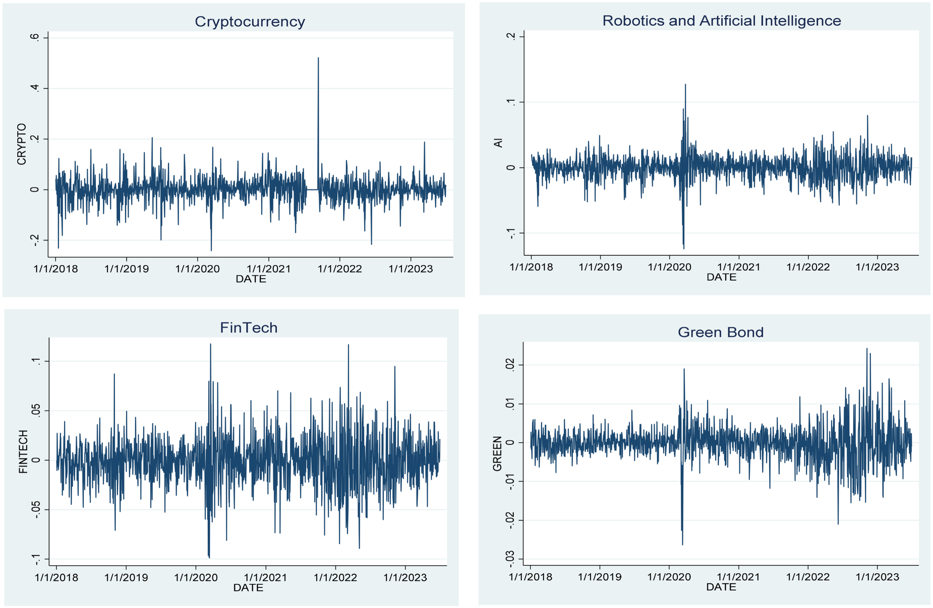
Modern Asset Returns Co-Movement.
Table 2 below shows that the asset returns on average are fluctuating before the crisis and post crisis. Whereas on average, all the asset returns are positive during the analysed crisis period with Gold scoring the highest average returns pre-crisis, Cryptocurrency scoring the highest average returns during the crisis and Commodities scoring the highest average returns post-crisis. Assets with the lowest average returns are FinTech pre-crisis, Green bond during the crisis and Precious metals post-crisis. Based on the standard deviations, the riskiest (more volatile) asset class is Cryptocurrency pre-crisis, Oil during the crisis and Cryptocurrency again post-crisis while the least risky asset class is Green bond across pre- during and post-crisis periods.
Descriptive Statistics.
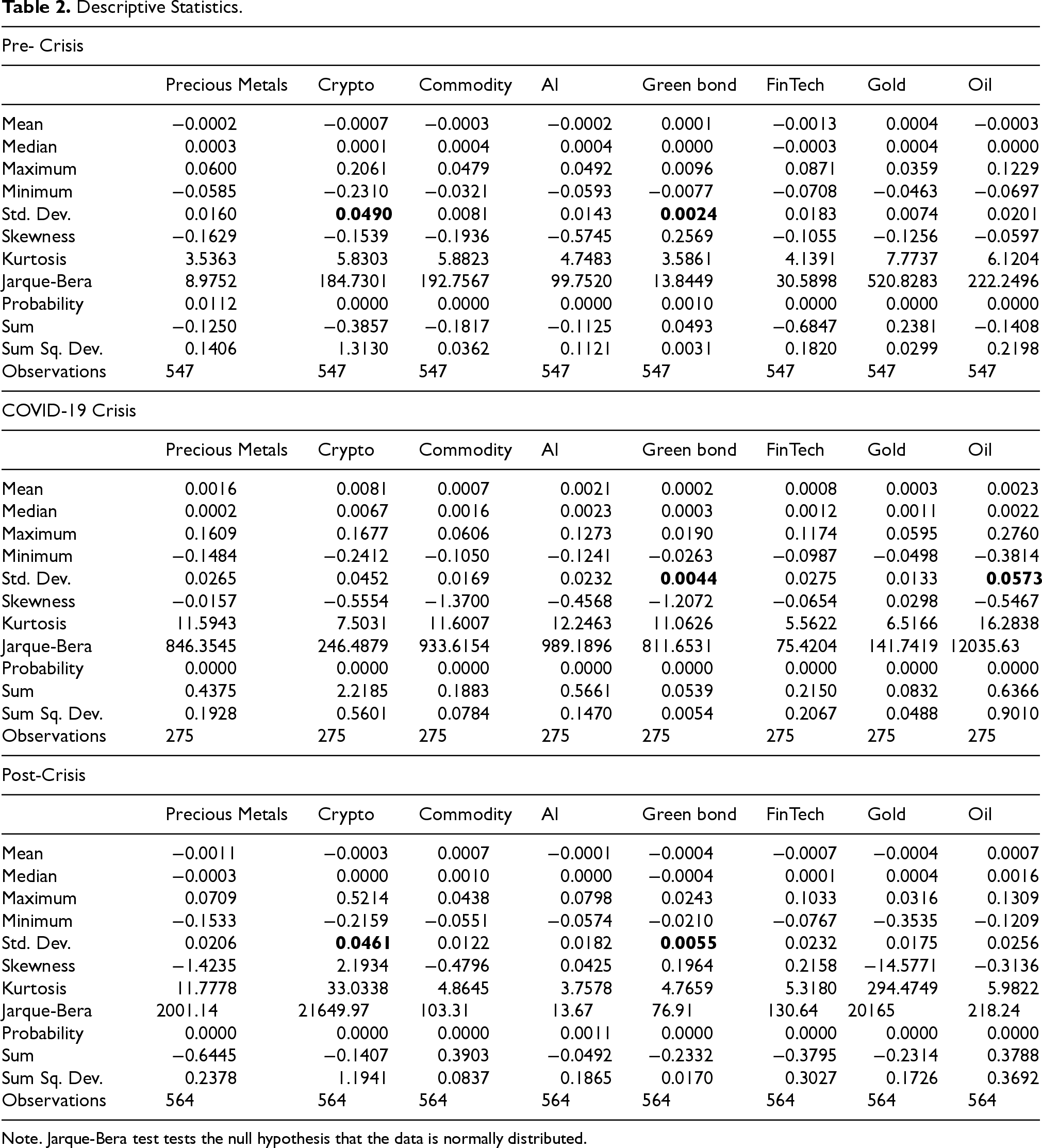
Descriptive Statistics.
Note. Jarque-Bera test tests the null hypothesis that the data is normally distributed.
The return volatility in Green bonds is relatively stable due to their defensive nature in investment portfolios. During the crisis, most assets, except for Green bonds and Gold, had negative skewness, meaning they commonly experienced sudden extreme negative returns. Conversely, Green bonds and Gold had positive skewness, indicating more positive shocks. All asset classes are prone to extreme low and high returns, as they follow a leptokurtic distribution, emphasizing the need to consider more than just mean-based connectedness when modelling their return relationships.
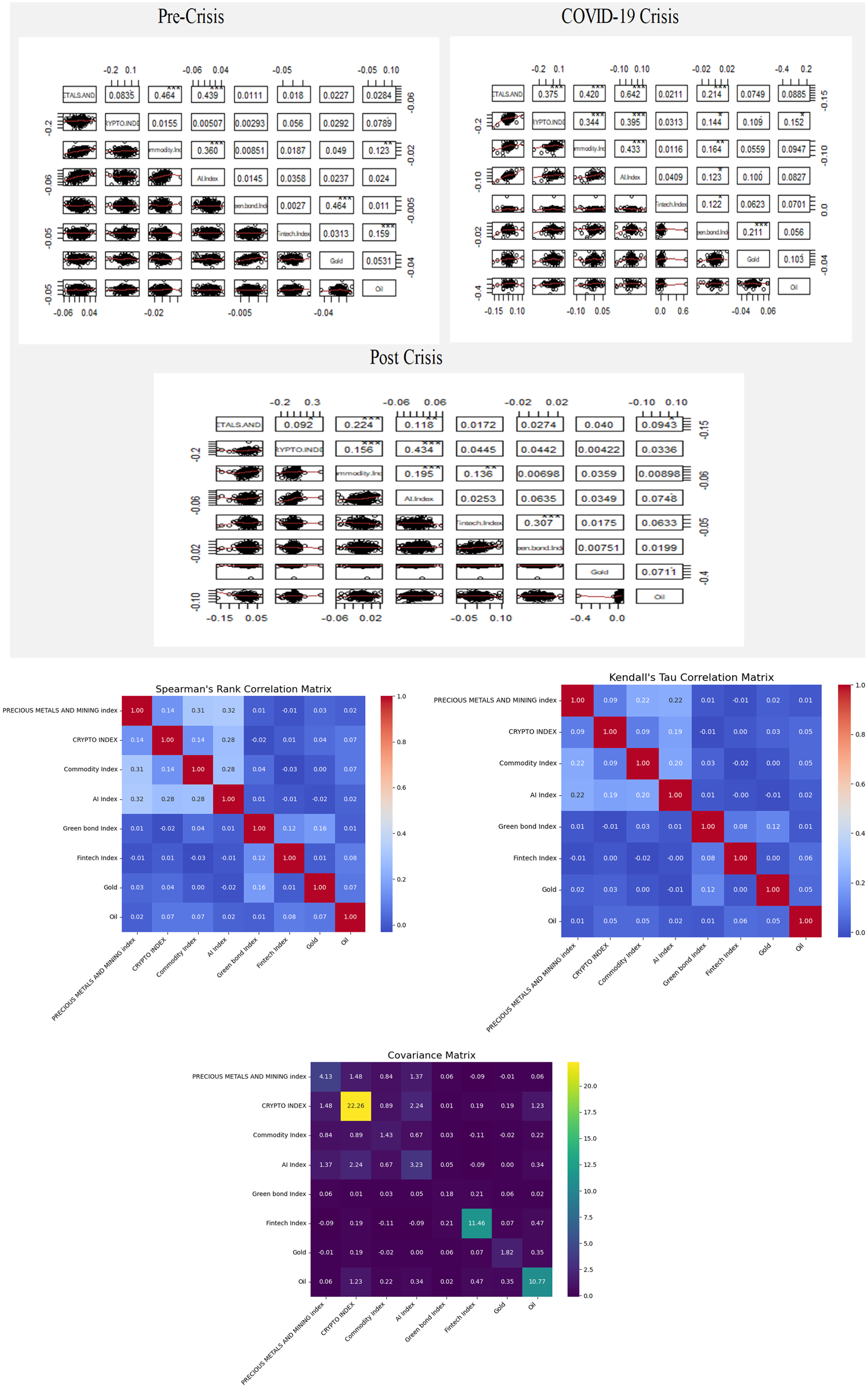
Table 3 and Figure 4 below present the pair-wise Pearson, Spearman's Rank and Kendall's Tau correlation coefficients matrix across the returns of modern and traditional asset classes. Positive correlation among the assets shows a complementary relationship between the assets while negative correlation signifies a substitution relationship between the asset classes. The strongest and significant correlation is observed during the COVID-19 crisis among Precious metals and AI (0.6436), showing a complementary relationship between traditional-modern asset pair. The lowest correlation is observed pre-COVID-19 crisis between Cryptocurrency and Green bond (0.0015), showing a weak complementary relation between modern-modern asset pair. It is also observed that the relationship between the asset's changes significantly across the crisis period, before, and after the crisis. Interestingly, during the crisis, there exists a positive (complementary) relationship between all the assets with exception between FinTech-Commodities and FinTech-AI pairs while a negative relationship (substitution) exists between these variables mentioned post-crisis. This analysis therefore signifies investors to be aware of the fluctuating relationship between these assets across different market conditions.
Pairwise Correlation Matrix Across Market Periods.
Pairwise Correlation Matrix Across Market Periods.
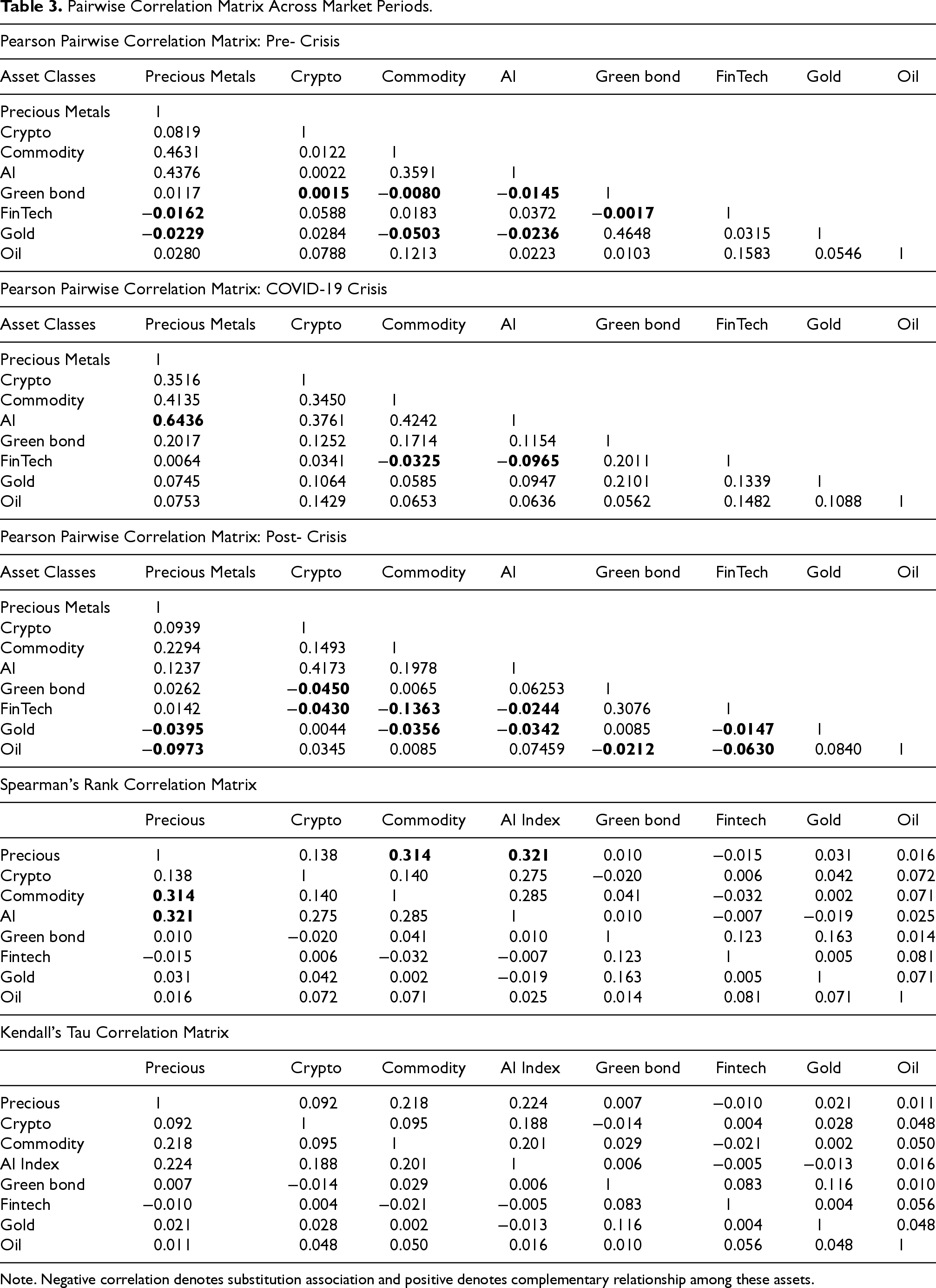
Note. Negative correlation denotes substitution association and positive denotes complementary relationship among these assets.
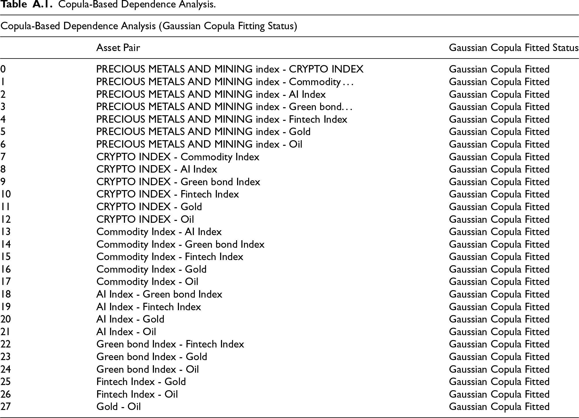
The successful fitting of Gaussian copulas across asset pairs indicates that an elliptical dependence structure may serve as a reasonable initial approximation under normal market conditions (see Appendix A). Covariance values, influenced by both correlation and volatility, reflect the absolute scale of co-movement, meaning assets with higher volatility may show elevated covariance even with moderate correlation. Comparing covariance and correlation heatmaps helps distinguish between relationships driven by pure correlation and those affected by price swings. Assets like FinTech, Gold, and Cryptocurrency, which exhibit low or negative correlations in Spearman's and Kendall's matrices, offer diversification benefits due to their tendency to move independently or inversely. The combined use of Spearman's Rho, Kendall's Tau, and Gaussian copulas reveals monotonic relationships and general dependence structures and further highlights the need for more advanced models of Quantile VAR to effectively capture tail-specific risk and dynamic connectedness.
The paper utilized a quantile-based VAR model of connectedness, following the approach outlined by Diebold and Yilmaz (2012, 2014). The quantile approach is utilized as an alternative to the standard mean-based approach in calculating the generalized connectedness index. It involves three specific quantiles: 0.10, 0.50, and 0.90, which correspond to different market conditions—bearish (0.10), normal (0.50), and bullish (0.90) volatility markets. The outcomes are presented in Tables 4 to 7. These values represent the variance in forecast errors of both traditional and modern asset returns. This variance arises from their own sources and from the innovations in other asset returns at various quantile levels. To simplify the analysis, it involves a bidirectional spillover index, denoted as “FROM” and “TO.” “FROM” indicates which assets receive return spillovers, while “TO” shows which assets transmit return spillovers. Consequently, positive net values indicate that an asset is a source of returns for others, while negative net values indicate that it receives returns from others.
Return Connectedness Estimated at the Mean of the Conditional Distribution.
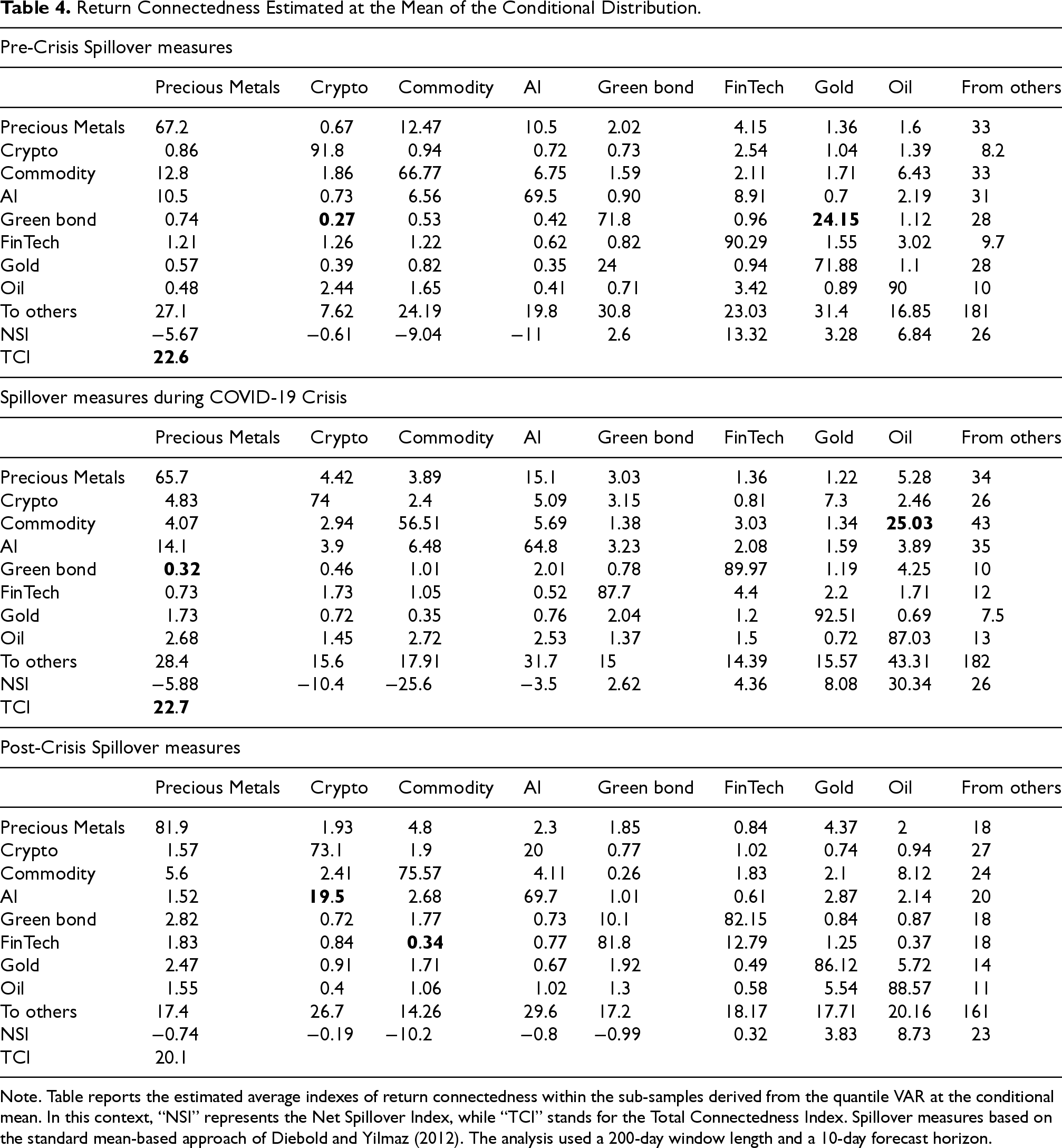
Return Connectedness Estimated at the Mean of the Conditional Distribution.
Note. Table reports the estimated average indexes of return connectedness within the sub-samples derived from the quantile VAR at the conditional mean. In this context, “NSI” represents the Net Spillover Index, while “TCI” stands for the Total Connectedness Index. Spillover measures based on the standard mean-based approach of Diebold and Yilmaz (2012). The analysis used a 200-day window length and a 10-day forecast horizon.
Return Connectedness Estimated at the Median of the Conditional Distribution.
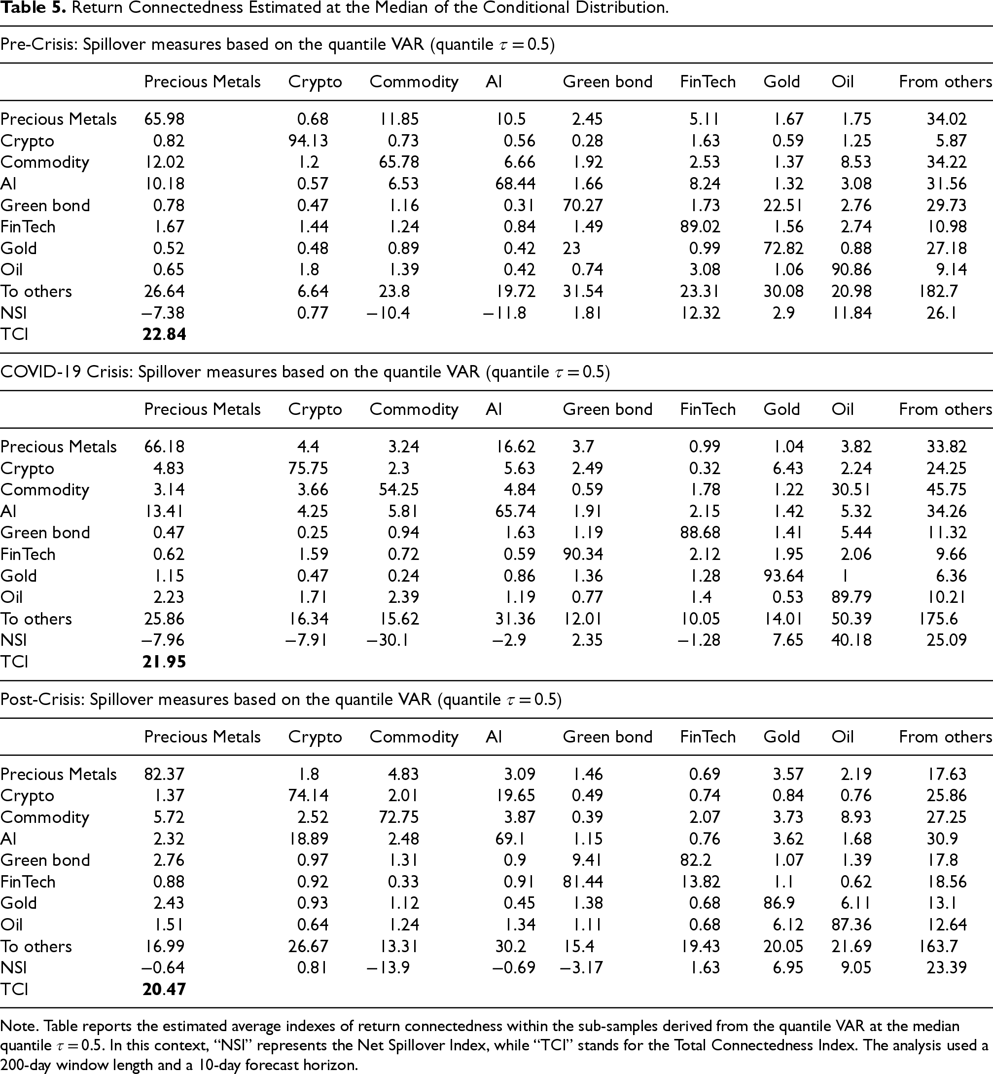
Note. Table reports the estimated average indexes of return connectedness within the sub-samples derived from the quantile VAR at the median quantile τ = 0.5. In this context, “NSI” represents the Net Spillover Index, while “TCI” stands for the Total Connectedness Index. The analysis used a 200-day window length and a 10-day forecast horizon.
Return Connectedness Based on the Quantile VAR at Lower Quantile τ = 0.1.
Note. Table reports the estimated average indexes of return connectedness within the sub-samples derived from the quantile VAR at the lower quantile τ = 0.1. The output for 0.05 is close to that of 0.10 and can be made available upon request. In this context, “NSI” represents the Net Spillover Index, while “TCI” stands for the Total Connectedness Index. The analysis used a 200-day window length and a 10-day forecast horizon.
Return Connectedness Based on the Quantile VAR at Upper Quantile τ = 0.90.
Note. Figures report the estimated average indexes of return connectedness within the sub-samples derived from the quantile VAR at upper quantile τ = 0.90. The output for 0.95 is close to that of 0.90 and can be made available upon request. In this context, “NSI” represents the Net Spillover Index, while “TCI” stands for the Total Connectedness Index. The analysis used a 200-day window length and a 10-day forecast horizon.
The paper estimates the quantile VAR model with the optimal lag order being 1 (Refer to Appendix B), selected based on the AIC to measure the return connectedness at the conditional median (quantile τ = 0.5), presented in Table 5. The connectedness measures estimated at the conditional mean and the median denote normal market conditions and are used as a reference for comparing the results of the connectedness at the upper and lower tails. Evidently, it is noted that when comparing the estimated results of at the mean connectedness in Table 4 to that of at the median connectedness in Table 5, the various connectedness measures at normal market conditions exhibit a high similarity respectively. This similarity is shown for example by TCI with conditional mean pre-crisis, during and post-crisis as (22.6, 22.7, and 20.1) which is not much different from the average TCI at the conditional median pre-crisis, during and post-crisis as (22.84, 21.95, and 20.47). The strongest return spillovers in the periods of pre-crisis, during and post-crisis are between Gold-Green Bond, Commodities-Oil and Cryptocurrency-AI, whereas the weakest return spillovers in the periods of pre-crisis, during and post-crisis are between Cryptocurrency-Green Bond, Precious Metals-Green Bond, and Commodities-FinTech
Average Connectedness During Bearish and Bullish Market Conditions
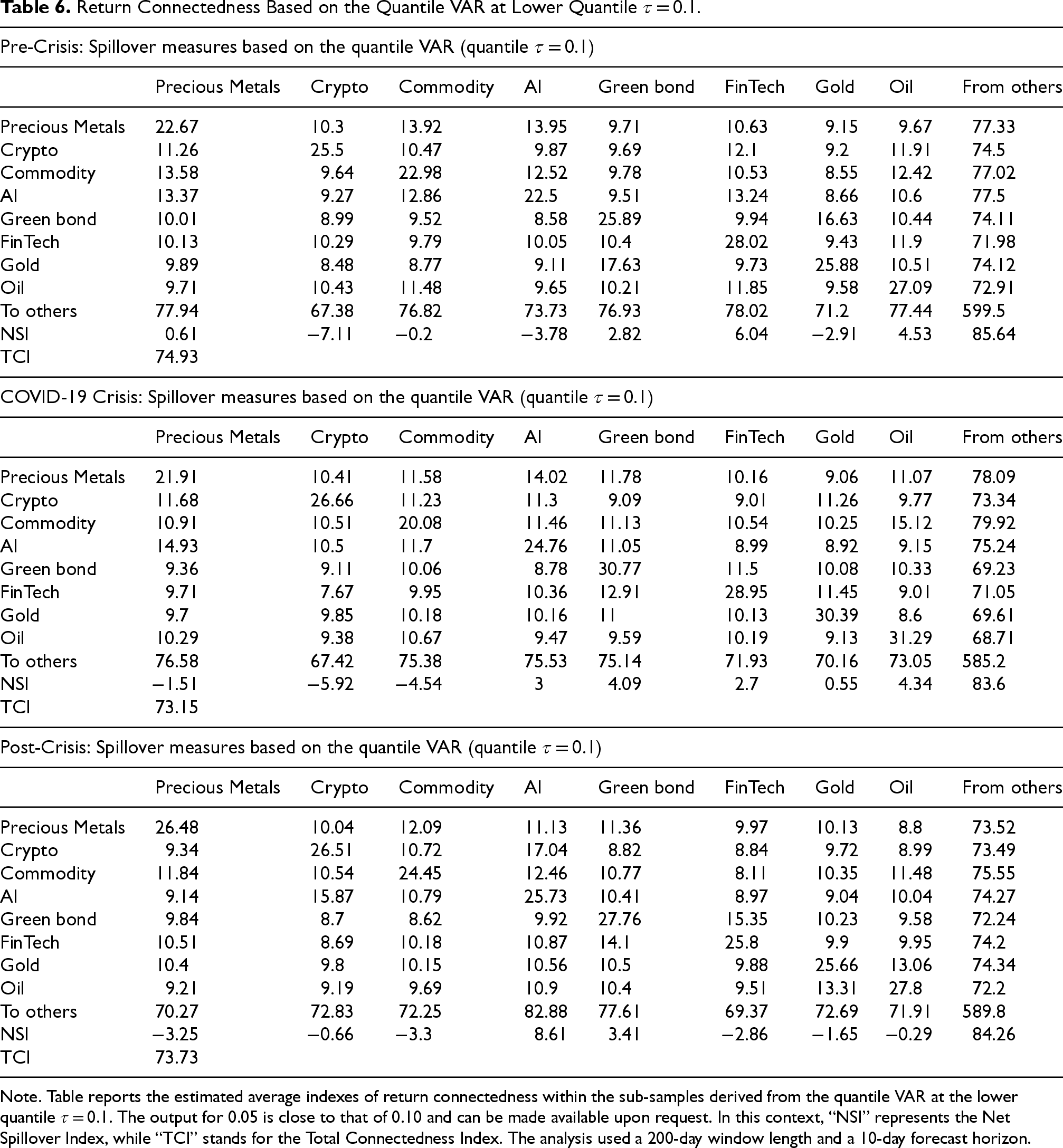
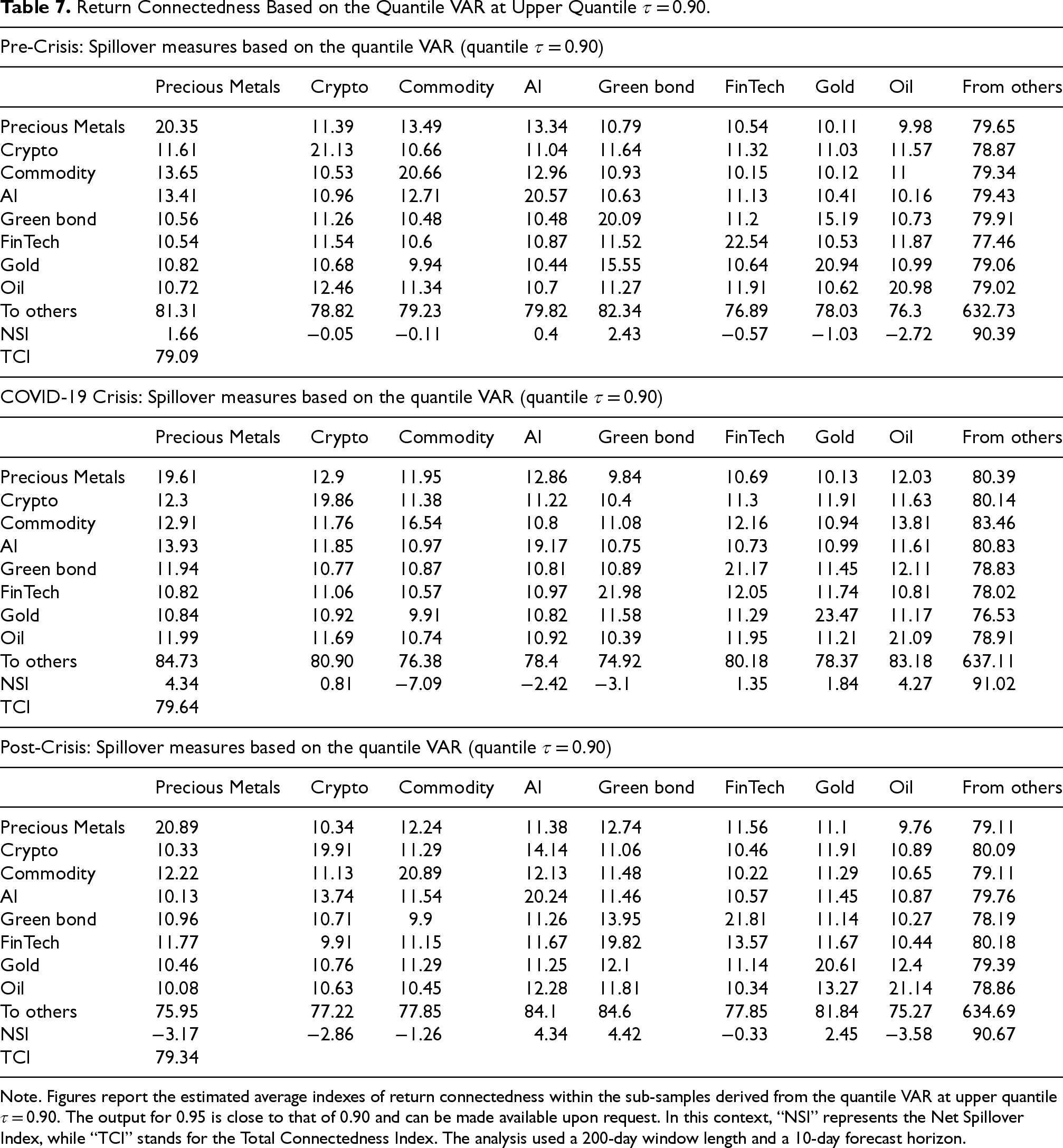
Tables 6 and 7 reports the evaluations of tail connectedness, both at the lower quantile (τ = 0.1) and the upper quantile (τ = 0.90), revealing a significant increase in directional return spillover among these asset classes, particularly during extreme market conditions. The results suggest that asset class interconnections intensify during periods of extreme market movements, both downturns and upswings. This is evidenced by the higher Total Connectedness Index (TCI) values observed at the lower (τ = 0.1) and upper (τ = 0.9) quantiles compared to the median (τ = 0.5), indicating that systemic linkages are more pronounced during extreme return conditions than during normal periods. Specifically, average TCI values at τ = 0.1 were 74.93, 73.15, and 73.73 during the pre-crisis, crisis, and post-crisis periods, respectively, while at τ = 0.9, they were even higher 79.09, 79.64, and 79.34 as compared to significantly lower values at the median quantile (22.84, 21.95, and 20.47). This pattern underscores the asymmetric nature of return spillovers across the distribution.
In terms of net spillover effects, FinTech, Gold, and Green Bonds were the primary recipients of shocks before the crisis. During the crisis, Oil and Precious Metals became the dominant receivers, while in the post-crisis period, AI and Green Bonds assumed this role. Across both bearish (τ = 0.1) and bullish (τ = 0.9) market conditions, Green Bonds, Gold, and FinTech consistently acted as net receivers of return spillovers, whereas Commodities, Cryptocurrencies, and to a lesser extent, Precious Metals served as net transmitters. Among these, Commodities and Cryptocurrencies were particularly robust in diffusing shocks, while AI and Precious Metals exhibited weaker transmission capabilities. Table 7 further confirms that Commodity, AI, and Cryptocurrency assets are persistent disseminators of extreme returns, making them critical for investors to monitor. Conversely, Green Bonds, Gold, and FinTech remain key absorbers of shocks, reinforcing their potential role in portfolio risk mitigation. Overall, while the magnitude of connectedness varies across quantiles, the directional roles of these assets remain stable, highlighting the importance of quantile-specific analysis in capturing the full spectrum of market dynamics.
Overall, from the discussion above, this paper finds that the relationships between traditional and modern assets exhibit greater strength during extreme circumstances compared to normal conditions. Using a quantile-based approach to analyse the linkage between traditional and modern assets, it becomes evident that shocks propagate more vigorously at the extreme tails of the conditional distribution as opposed to the conditional mean and median. Additionally, the spillover patterns observed at the tails differ from those at the mean and median. Notably, some traditional assets consistently act as sources of spillover in the analysis, while a few modern assets, such as AI and Cryptocurrency, appear to transmit spillovers to the modern assets markets.
Network Analysis
This paper visually shows the network connectedness among the asset's classes across different quantiles, in Figures 5 to 7, involving assessment of network return connectedness at different quantiles: the middle quantile (τ = 0.5), lower quantile (τ = 0.1), and upper quantile (τ = 0.90). The node size reflects the extent of net return spillover, while the node colour distinguishes between assets as net receivers (Green) or net transmitters (Red) of return shocks. The arrow edge thickness indicates the strength of spillover connections between assets.
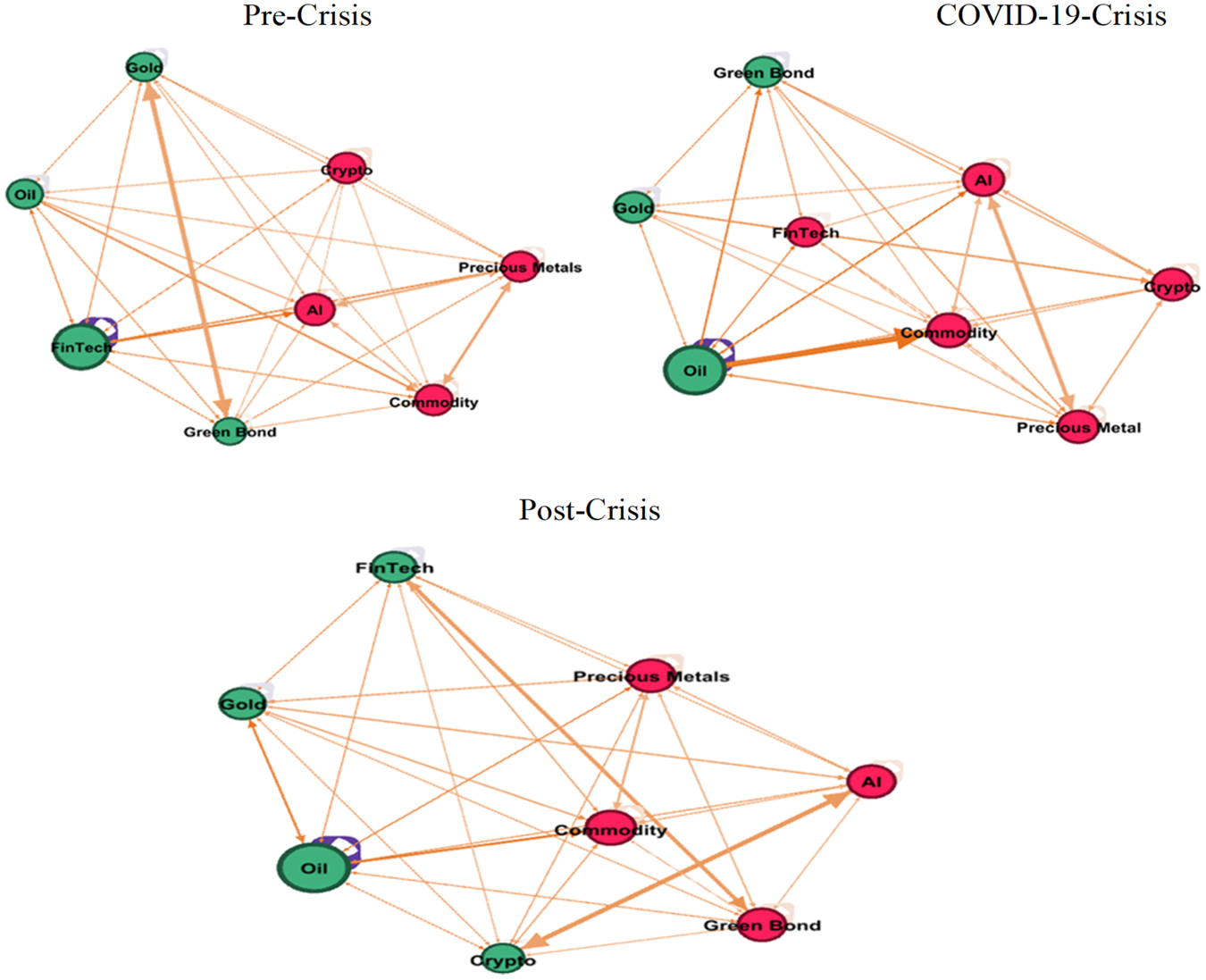
Network Connectedness Based on the Quantile VAR (Quantile τ = 0.5).
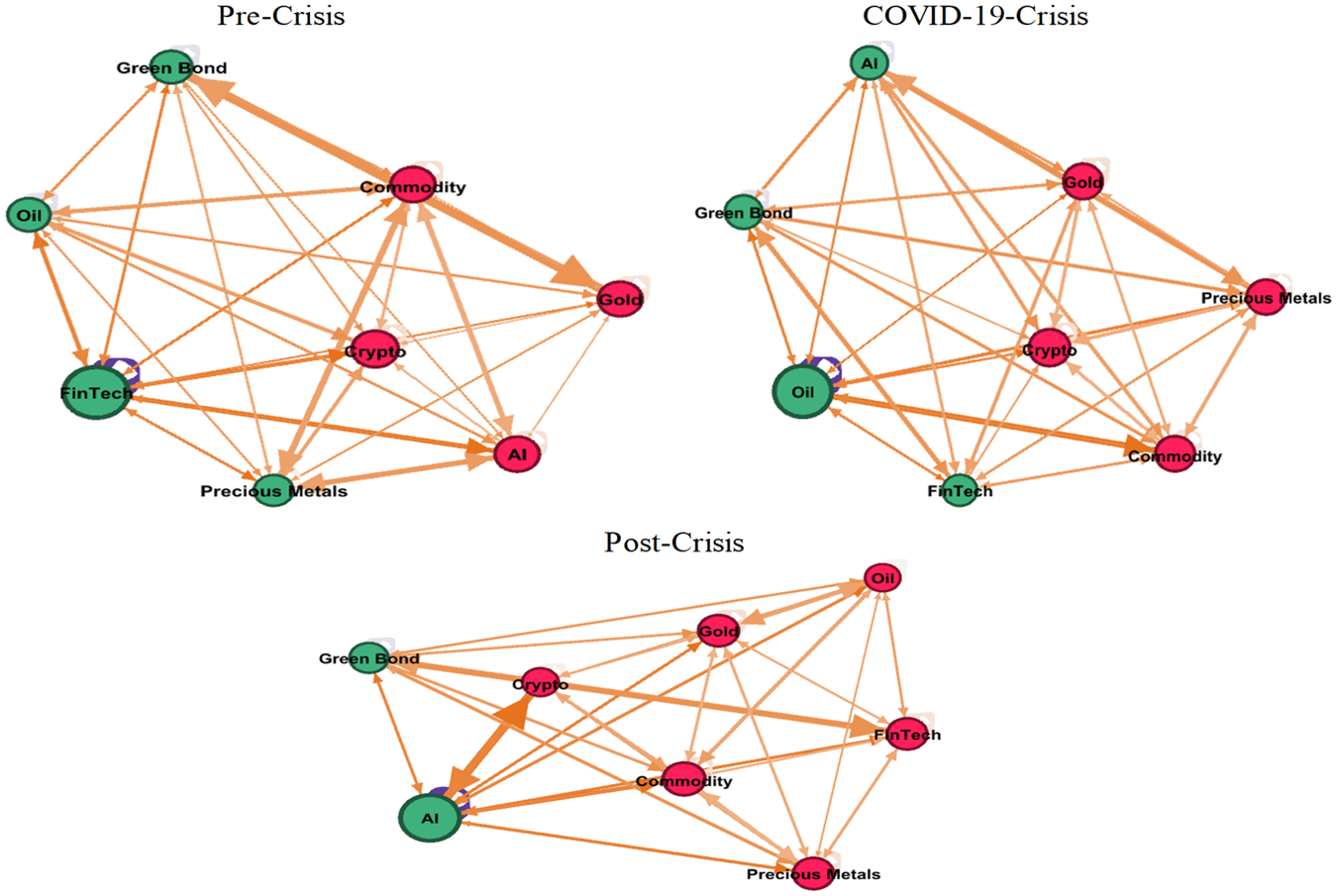
Network Connectedness Based on the Quantile VAR (Quantile τ = 0.1).
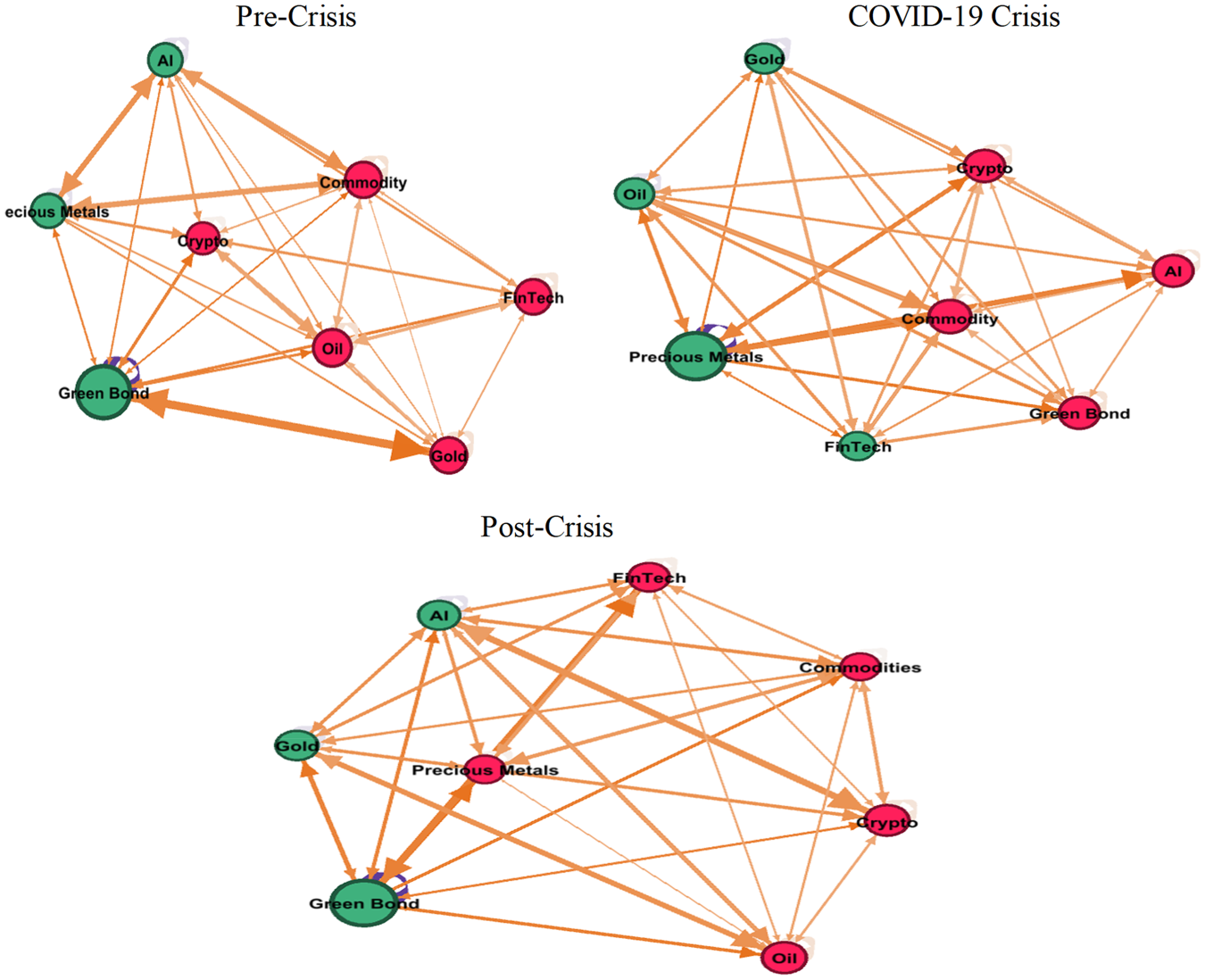
Network Connectedness Based on the Quantile VAR (Quantile τ = 0.90).
In Figure 5, during normal market conditions (τ = 0.5), the role of assets in terms of receiving or transmitting return spillover effects varies. Pre-crisis, Crude Oil, Green Bond, FinTech, Gold, and Cryptocurrency are net receivers, while Precious Metals, Commodity, and AI are net transmitters. During the COVID-19 crisis, Green Bond, Gold, and Oil become net receivers, whereas Precious Metals, Cryptocurrency, Commodity, AI, and FinTech are net transmitters. Post-crisis, Cryptocurrency, FinTech, Gold, and Oil are net receivers, while Precious Metals, Commodity, Green Bond, and AI are net transmitters.
Figure 6 demonstrates network connectedness during bear market conditions (τ = 0.1). Pre-crisis, Precious Metals, Green Bond, FinTech, and Oil are net receivers, and Cryptocurrency, Commodity, Gold, and AI are net transmitters. During the COVID-19 crisis, Green Bond, AI, FinTech, and Oil are net receivers, while Precious Metals, Cryptocurrency, Commodity, and Gold are net transmitters. Post-crisis, only Green Bond and AI are net receivers, while Precious Metals, Commodity, Cryptocurrency, FinTech, Gold, and Oil are net transmitters.
Figure 7 represents connectedness in bear market conditions (τ = 0.90). Pre-COVID-19 crisis, Precious Metals, Green Bond, and AI are net receivers, with Cryptocurrency, Commodity, FinTech, Gold, and Oil being net transmitters. During the COVID-19 crisis, Green Bond, AI, FinTech, and Gold become net receivers, while Precious Metals, Cryptocurrency, Commodity, and Oil are net transmitters. Post-crisis, Green Bond, AI, and Gold are net receivers, while Precious Metals, Cryptocurrency, Commodity, FinTech, and Oil are net transmitters.
The analysis indicates that Green Bond, FinTech, Gold, and Oil are strong receivers of return shocks pre-crisis and during the crisis, while Precious Metals and AI are weak receivers. Post-crisis, Gold and Oil continue as strong receivers, and Precious Metals, FinTech, and AI remain weak receivers. In terms of transmitters, Commodity and Cryptocurrency are strong diffusers of return shocks across all periods, while Precious Metals and AI are weak transmitters. Figures 6 and 7 illustrate the consistent pattern of these assets with Green Bond, FinTech, Oil, and Gold absorbing shocks and Commodity, Precious Metals, and Cryptocurrencies transmitting shocks.
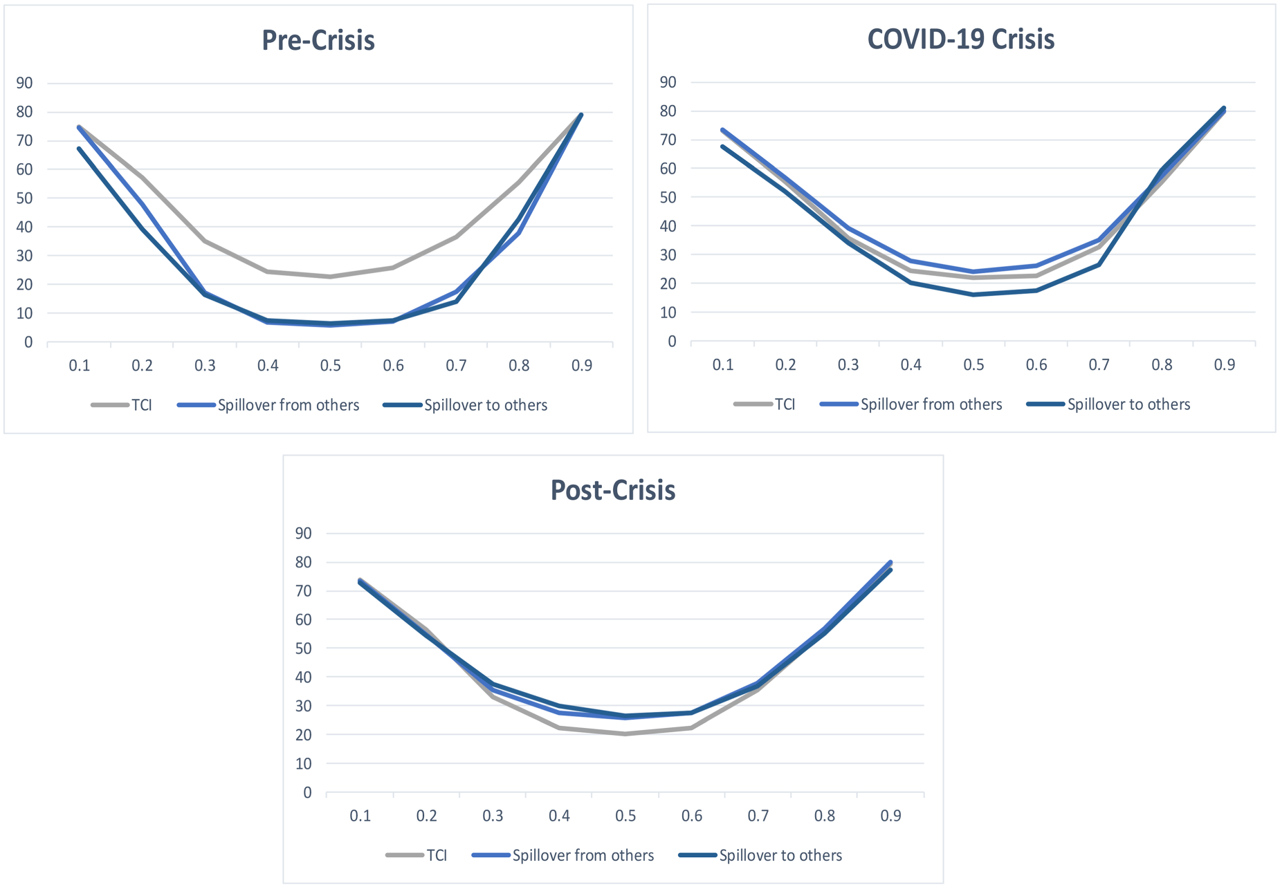
Figure 8 shows the time-varying TCI under heterogenous market conditions, “spillover from others” index, and “spillover to others” index of the modern and traditional asset markets across different quantiles. From the graphical representation, the vertical axis represents the total spillover, and the horizontal axis denotes the conditional quantiles of different market conditions.
Variations in the Return Connectedness Measures Across Various Quantiles.
The time-varying TCI exhibits a distinctive pattern resembling an inverted bell curve, wherein the highest spillover occurs during extreme conditions, and it takes on a U-shaped form spanning from 10% to 90%. Notably, it elevates during periods of both extreme market conditions, whether bearish or bullish, and declines to its minimum level during normal market conditions. This consistent and symmetrical pattern persists across all examined sub-periods, encompassing both the upper and lower tails of the TCI. This symmetrical pattern underscores the equal significance of substantial positive or negative return shocks in driving the spillover effects within this classification. Furthermore, the spillover effects between modern and traditional asset markets demonstrate a relative symmetry in response to both profoundly positive and negative returns.
To validate the estimated results, this paper further assesses the sensitivity of the findings by modifying few specifications to re-evaluate connectedness at different quantiles. This involves adjustments to the rolling window size and forecast horizon as this paper presented variations to the analyses. Initially, the analysis used a 200-day window length and a 10-day forecast horizon. To gauge sensitivity, the paper has now incorporated a 250-day window length and a 5-day forecast horizon, re-estimating the connectedness models across different quantiles. The results indicate a slight decrease in the TCI, while the primary dynamics, which are of utmost interest, remain relatively consistent. Moreover, this pattern persists when the models are re-evaluated at both the conditional mean and median, as presented in Tables A.1 to D.4 in the Appendix. During extreme market conditions, as exemplified in Tables D.5 and D.6 for bull and bearish scenarios, total spillovers remain notably high in the tails, significantly surpassing the levels observed in the mean and median, consistent with the initial findings in the primary estimation. Similarly, this asymmetric feature remains constant even when the relative tail dependence is computed with different window lengths. In essence, these adjustments in the analysis parameters highlight the robustness and reliability of the observed asymmetric features across various quantiles and window lengths. Overall, all these analyses indicate that the findings are robust and not sensitive to specifications of the size of the window and the forecast horizon selected for estimation.
Portfolio Implications
The findings highlighted the significance of return spillover effects among different asset categories, with the intensity varying across quantiles within the conditional distribution. More extreme shocks tend to have broader impacts. For investors and portfolio managers, this suggests a need to consider risks associated with extreme events and adjust portfolio weightings to mitigate these risks. The paper further analyses a dynamic portfolio approach to help minimize potential losses due to increased return connectedness, particularly in the left tail of the distribution.
Table 8 provided below displays the downside risk assessment of the portfolio design, as measured by VaR, CVaR, and ES, for each asset within both traditional and modern samples. These risk assessments are conducted at confidence levels of 95% and 99% and span the pre-crisis, COVID-19 crisis, and post-crisis periods. The portfolio design entails various combinations of asset pairs, encompassing traditional-modern, modern-modern, and traditional-traditional asset classes across the sub-samples. These combinations aim to determine the optimal portfolio weights based on the degree of connectedness between traditional and modern assets, ranging from 0 for less favourable asset classes to 1 for more favourable asset classes, within the sub-samples across diverse market conditions.
VaR, CVaR and ES Tail Risk Measures Analysis.
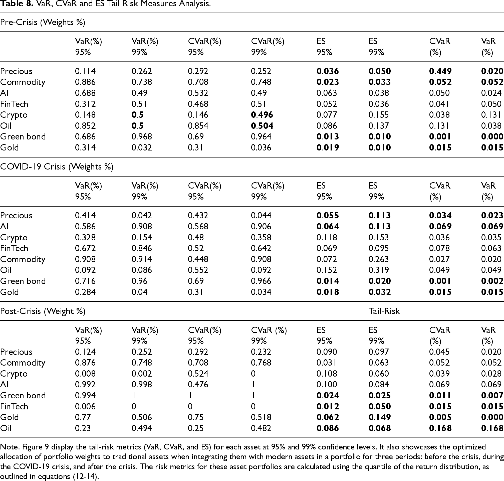
VaR, CVaR and ES Tail Risk Measures Analysis.
Note. Figure 9 display the tail-risk metrics (VaR, CVaR, and ES) for each asset at 95% and 99% confidence levels. It also showcases the optimized allocation of portfolio weights to traditional assets when integrating them with modern assets in a portfolio for three periods: before the crisis, during the COVID-19 crisis, and after the crisis. The risk metrics for these asset portfolios are calculated using the quantile of the return distribution, as outlined in equations (12-14).
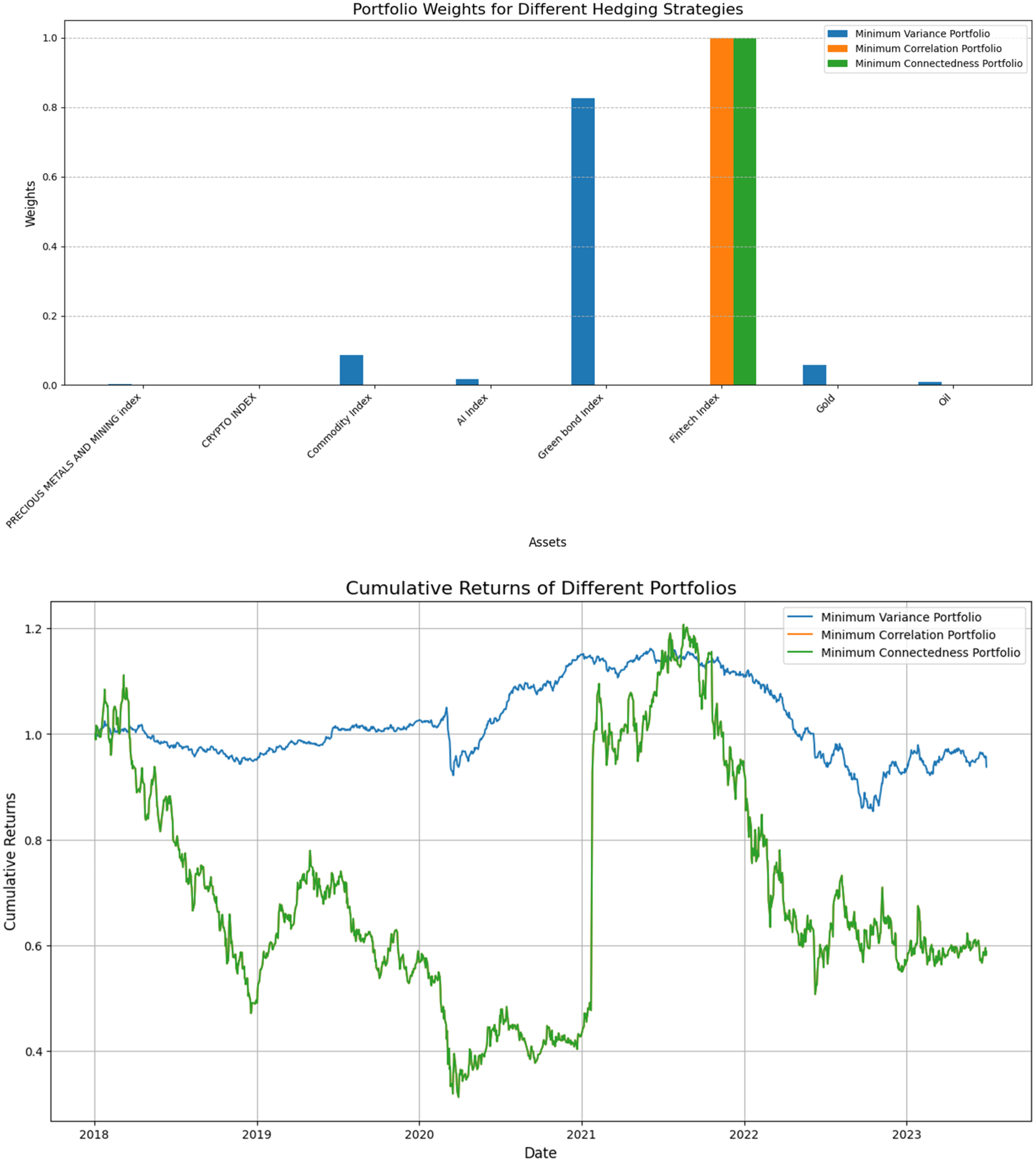
Portfolio Weights and Comparative Performance Across Portfolios.
Before the COVID-19 pandemic, optimal asset allocation varied. For instance, between Green bonds-Gold, the optimal allocation was R0.686 for Green bonds and R0.314 for Gold, favouring Green bonds. In the case of the Cryptocurrency-Oil pairing, it was optimal to allocate R0.50 to Cryptocurrency and R0.50 to crude Oil. Similarly, AI-FinTech portfolios suggested an allocation of 0.532 for AI and 0.468 for FinTech. This pre-pandemic strategy favoured modern assets over traditional assets in portfolios.
During the COVID-19 pandemic, the optimal asset allocation within various portfolios also differed. The optimal allocation between Precious metals-AI ranged from 0.432 for Precious metals to 0.568 for AI. For the Green bond-Gold pairing, it was optimal to allocate R0.716 to Green bonds and R0.284 to Gold. A similar allocation was recommended for the Cryptocurrency-FinTech portfolio during the crisis, with 0.328 for Cryptocurrency and 0.672 for FinTech. These allocations aimed to balance risk and return in extreme market conditions. However, it's essential to be cautious about the specific type of modern asset, as Cryptocurrency was found to be highly risky during the crisis. After the COVID-19 pandemic, the optimal allocation between Green bonds-FinTech was 1 for Green bonds and 0 for FinTech, indicating an emphasis on Green bonds. In the Cryptocurrency-AI portfolio, the optimal allocation was R0.008 for Cryptocurrency and R0.992 for AI. This post-crisis allocation strategy aimed to maximize returns with lower risk, suggesting a preference for AI, Green bonds, Gold, and Commodity in portfolios.
In summary, before the COVID-19 crisis, optimal allocations in portfolios were higher compared to the post-crisis period. Hedging costs were lowest during the pandemic for certain portfolios but highest for Commodity-Oil portfolios. The optimal asset weights in dynamic portfolios varied across pre-crisis, crisis, and post-crisis periods, suggesting that investors should lean towards portfolios that combine modern and traditional assets, particularly those with lower relative risk like Green bonds, AI, FinTech, and Gold. During the crisis, ideal allocations to modern assets decreased due to increased risk, and after the crisis, recommended weights for traditional assets were generally below 50%, indicating a need for reduced holdings in AI, FinTech, and Cryptocurrency to mitigate potential risks. These adjustments align with risk metrics showing higher tail risk in these assets over the analysed period.
The overall findings reveals that extreme return shocks spread differently through interconnected modern and traditional asset markets. It highlights asymmetry and heightened return spillovers, especially in the tails of the distribution, challenging mean-based literature. Asymmetric asset dependencies may be attributed to liquidity shocks, volatility clustering, and changes in investor sentiment during market anxiety. Bearish conditions typically strengthen assets correlations as investors liquidate positions across asset classes; leading to “flight-to-safety” effects. Traditional assets are inclined to steadier co-movements in normal periods due to their deeper liquidity and institutional participation, whereas modern assets including cryptocurrencies—are more speculative and emotion-driven, intensifying asymmetries, particularly in extreme market conditions.
This approach, incorporating the context of the COVID-19 outbreak, provides unique insights into connectedness dynamics. It suggests that assessing connectedness only at conditional mean and median levels misses the full picture during periods of significant shocks. Active portfolio management, considering both modern and traditional assets, can effectively mitigate tail-risk compared to a passive buy-and-hold strategy, although the extent of this benefit depends on specific assets, market conditions, and choice of risk measures.
This study undertakes a comparative empirical analysis of three portfolio optimization frameworks Minimum Variance Portfolio (MVP), Minimum Correlation Portfolio (MCP), and Minimum Connectedness Portfolio (MCoP) to assess their respective capacities for managing risk and enhancing portfolio resilience. The primary aim is to evaluate how effectively each strategy mitigates exposure to systemic market disruptions, particularly those triggered by the COVID-19 pandemic.
The above findings suggest that while MVP remains effective within conventional asset groupings due to its focus on minimizing volatility through covariance structures, MCP and MCoP demonstrate superior performance in managing risk across modern asset classes such as FinTech and green bonds. These latter strategies leverage diversification and network-based risk metrics to achieve broader volatility reduction, especially in environments characterized by high uncertainty and structural shifts.
The empirical results align with Broadstock et al. (2022), who emphasized the benefits of constructing portfolios with limited interconnectivity between green and traditional bonds, thereby reducing contagion risk. Similarly, Xia et al. (2022) identified specific green equities as potential safe-haven assets, capable of serving as effective hedging instruments during periods of market stress. Collectively, these findings underscore the evolving nature of portfolio optimization, where traditional variance-based models are increasingly complemented or even supplanted by approaches that incorporate correlation structures and systemic interdependencies. The choice of methodology should thus reflect not only investor preferences but also the structural characteristics of the asset universe and prevailing macroeconomic conditions.
This paper explored how modern technology-driven assets affect portfolio diversification, especially during the COVID-19 pandemic. It reveals that returns of modern and traditional assets are more connected during extreme market conditions, both in the upper and lower tails, compared to normal market conditions. This connection is asymmetric, meaning both positive and negative shocks matter. Modern assets like Green bonds, AI, Gold, and FinTech tend to receive shocks, while traditional assets like Precious metals, Commodities, and Oil transmit shocks, with modern assets playing a more significant role at the extreme tails. Interestingly, the COVID-19 crisis mainly impacted the lower and middle tails of connectedness. For portfolios, it suggests allocating funds to Green bonds, AI, Commodities, and Oil during crises to reduce risks. Cryptocurrencies acted as safe havens before the crisis but lost this status during COVID-19.
The analysis reveals that asset class connectedness intensifies during periods of extreme market conditions, specifically at the lower (τ = 0.1) and upper (τ = 0.9) quantiles of the return distribution, which correspond to extreme negative and positive return scenarios, respectively. This is evidenced by the elevated Total Connectedness Index (TCI) values at these quantiles compared to the median (τ = 0.5), which represents typical market conditions. For instance, TCI values at τ = 0.1 and τ = 0.9 consistently exceed those at τ = 0.5 across pre-crisis, crisis, and post-crisis periods, indicating that systemic linkages are more pronounced during market stress or exuberance.
Network analysis highpoints that FinTech, Gold, and Green Bonds were net receivers of return spillovers prior to the crisis, while Oil and Precious Metals assumed this role during the crisis, and AI and Green Bonds post-crisis. Across both bearish and bullish regimes, Green Bonds, Gold, and FinTech consistently absorb shocks, whereas Commodities, Cryptocurrencies, and to a lesser extent, Precious Metals act as net transmitters. Importantly, the roles of these assets are stable across quantiles, reinforcing their strategic relevance in portfolio construction.
These findings highlight the importance of monitoring technology asset portfolios, particularly during extreme market conditions, due to significant interconnectedness in returns. Traditional assets tend to transmit shocks, requiring thorough analysis. A dynamic approach to minimize tail-risk is recommended over passive strategies. Policymakers should use quantile-based measures to understand risk transmission and reduce economic policy uncertainty. Implications include diversification and safe-haven attributes of technology assets for investors. Traders in the technology sector can refine strategies, and a rotation strategy is advised for portfolio resilience. However, the focus on the COVID-19 crisis limits its generalizability, and future research should expand the sample and consider other crises and time periods. Increasing the portfolio size and using disaggregated indexes could enhance insights. Exploring global uncertainties and macroeconomic variables’ impact on technology assets is also suggested.
Footnotes
Funding
The authors received no financial support for the research, authorship, and/or publication of this article.
Declaration of Conflicting Interests
The authors declared no potential conflicts of interest with respect to the research, authorship, and/or publication of this article.
Appendix A
Copula-Based Dependence Analysis.
| Copula-Based Dependence Analysis (Gaussian Copula Fitting Status) | ||
|---|---|---|
| Asset Pair | Gaussian Copula Fitted Status | |
| 0 | PRECIOUS METALS AND MINING index - CRYPTO INDEX | Gaussian Copula Fitted |
| 1 | PRECIOUS METALS AND MINING index - Commodity … | Gaussian Copula Fitted |
| 2 | PRECIOUS METALS AND MINING index - AI Index | Gaussian Copula Fitted |
| 3 | PRECIOUS METALS AND MINING index - Green bond… | Gaussian Copula Fitted |
| 4 | PRECIOUS METALS AND MINING index - Fintech Index | Gaussian Copula Fitted |
| 5 | PRECIOUS METALS AND MINING index - Gold | Gaussian Copula Fitted |
| 6 | PRECIOUS METALS AND MINING index - Oil | Gaussian Copula Fitted |
| 7 | CRYPTO INDEX - Commodity Index | Gaussian Copula Fitted |
| 8 | CRYPTO INDEX - AI Index | Gaussian Copula Fitted |
| 9 | CRYPTO INDEX - Green bond Index | Gaussian Copula Fitted |
| 10 | CRYPTO INDEX - Fintech Index | Gaussian Copula Fitted |
| 11 | CRYPTO INDEX - Gold | Gaussian Copula Fitted |
| 12 | CRYPTO INDEX - Oil | Gaussian Copula Fitted |
| 13 | Commodity Index - AI Index | Gaussian Copula Fitted |
| 14 | Commodity Index - Green bond Index | Gaussian Copula Fitted |
| 15 | Commodity Index - Fintech Index | Gaussian Copula Fitted |
| 16 | Commodity Index - Gold | Gaussian Copula Fitted |
| 17 | Commodity Index - Oil | Gaussian Copula Fitted |
| 18 | AI Index - Green bond Index | Gaussian Copula Fitted |
| 19 | AI Index - Fintech Index | Gaussian Copula Fitted |
| 20 | AI Index - Gold | Gaussian Copula Fitted |
| 21 | AI Index - Oil | Gaussian Copula Fitted |
| 22 | Green bond Index - Fintech Index | Gaussian Copula Fitted |
| 23 | Green bond Index - Gold | Gaussian Copula Fitted |
| 24 | Green bond Index - Oil | Gaussian Copula Fitted |
| 25 | Fintech Index - Gold | Gaussian Copula Fitted |
| 26 | Fintech Index - Oil | Gaussian Copula Fitted |
| 27 | Gold - Oil | Gaussian Copula Fitted |
Appendix B
Optimal Lag Order Selection.
| Metric | Value |
|---|---|
| Optimal Lag Order (based on BIC) | 1 |
| Chosen Forecast Horizon | 30 days |
| BIC for Lag 1 | {{bic_values[0]:.4f}} |
| BIC for Lag 2 | {{bic_values[1]:.4f}} |
| BIC for Lag 3 | {{bic_values[2]:.4f}} |
| BIC for Lag 4 | {{bic_values[3]:.4f}} |
| BIC for Lag 5 | {{bic_values[4]:.4f}} |
| BIC for Lag 6 | {{bic_values[5]:.4f}} |
| BIC for Lag 7 | {{bic_values[6]:.4f}} |
| BIC for Lag 8 | {{bic_values[7]:.4f}} |
| BIC for Lag 9 | {{bic_values[8]:.4f}} |
| BIC for Lag 10 | {{bic_values[9]:.4f}} |
Appendix C
For each risk measure, the portfolio optimization problem is formulated as follows:
Minimize the portfolio's tail risk (VaR, CVaR, or ES) at a specified confidence level α.
Full investment:
No short selling:
Following Rockafellar and Uryasev (2000), the CVaR minimization problem is formulated as:
Where
VaR optimization is less tractable due to its non-convexity. We approximate the VaR minimization using a quantile-based approach:
Expected Shortfall is defined as the expected loss beyond the VaR threshold:
This is solved using a two-step procedure: Estimate VaR at level α and compute the mean of losses exceeding VaR. Optimization is performed using numerical methods over empirical distribution. All optimization problems were implemented in Python using historical daily returns across the period of review to generate scenarios. Confidence levels of 95% and 99% were tested.
Appendix D
Spillover Measures Based on Upper Quantile VAR (Quantile τ = 0.90).
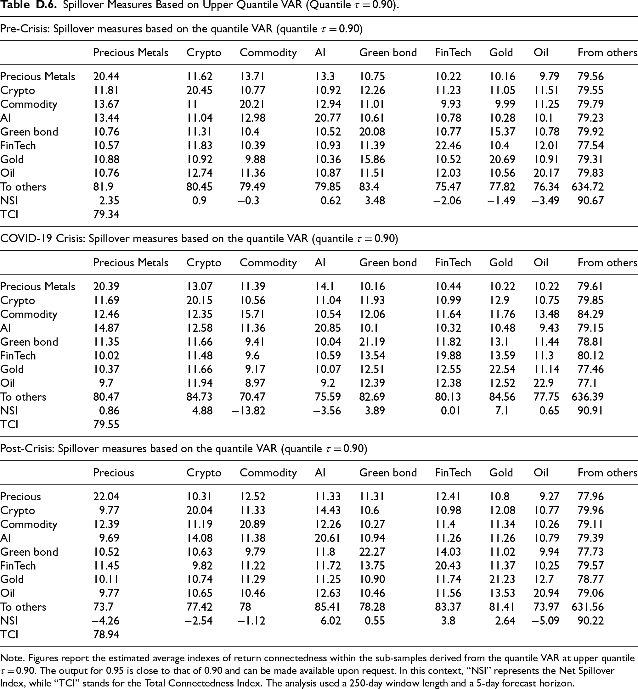
| Pre-Crisis: Spillover measures based on the quantile VAR (quantile τ = 0.90) | |||||||||
|---|---|---|---|---|---|---|---|---|---|
| Precious Metals | Crypto | Commodity | AI | Green bond | FinTech | Gold | Oil | From others | |
| Precious Metals | 20.44 | 11.62 | 13.71 | 13.3 | 10.75 | 10.22 | 10.16 | 9.79 | 79.56 |
| Crypto | 11.81 | 20.45 | 10.77 | 10.92 | 12.26 | 11.23 | 11.05 | 11.51 | 79.55 |
| Commodity | 13.67 | 11 | 20.21 | 12.94 | 11.01 | 9.93 | 9.99 | 11.25 | 79.79 |
| AI | 13.44 | 11.04 | 12.98 | 20.77 | 10.61 | 10.78 | 10.28 | 10.1 | 79.23 |
| Green bond | 10.76 | 11.31 | 10.4 | 10.52 | 20.08 | 10.77 | 15.37 | 10.78 | 79.92 |
| FinTech | 10.57 | 11.83 | 10.39 | 10.93 | 11.39 | 22.46 | 10.4 | 12.01 | 77.54 |
| Gold | 10.88 | 10.92 | 9.88 | 10.36 | 15.86 | 10.52 | 20.69 | 10.91 | 79.31 |
| Oil | 10.76 | 12.74 | 11.36 | 10.87 | 11.51 | 12.03 | 10.56 | 20.17 | 79.83 |
| To others | 81.9 | 80.45 | 79.49 | 79.85 | 83.4 | 75.47 | 77.82 | 76.34 | 634.72 |
| NSI | 2.35 | 0.9 | −0.3 | 0.62 | 3.48 | −2.06 | −1.49 | −3.49 | 90.67 |
| TCI | 79.34 | ||||||||
| COVID-19 Crisis: Spillover measures based on the quantile VAR (quantile τ = 0.90) | |||||||||
| Precious Metals | Crypto | Commodity | AI | Green bond | FinTech | Gold | Oil | From others | |
| Precious Metals | 20.39 | 13.07 | 11.39 | 14.1 | 10.16 | 10.44 | 10.22 | 10.22 | 79.61 |
| Crypto | 11.69 | 20.15 | 10.56 | 11.04 | 11.93 | 10.99 | 12.9 | 10.75 | 79.85 |
| Commodity | 12.46 | 12.35 | 15.71 | 10.54 | 12.06 | 11.64 | 11.76 | 13.48 | 84.29 |
| AI | 14.87 | 12.58 | 11.36 | 20.85 | 10.1 | 10.32 | 10.48 | 9.43 | 79.15 |
| Green bond | 11.35 | 11.66 | 9.41 | 10.04 | 21.19 | 11.82 | 13.1 | 11.44 | 78.81 |
| FinTech | 10.02 | 11.48 | 9.6 | 10.59 | 13.54 | 19.88 | 13.59 | 11.3 | 80.12 |
| Gold | 10.37 | 11.66 | 9.17 | 10.07 | 12.51 | 12.55 | 22.54 | 11.14 | 77.46 |
| Oil | 9.7 | 11.94 | 8.97 | 9.2 | 12.39 | 12.38 | 12.52 | 22.9 | 77.1 |
| To others | 80.47 | 84.73 | 70.47 | 75.59 | 82.69 | 80.13 | 84.56 | 77.75 | 636.39 |
| NSI | 0.86 | 4.88 | -13.82 | -3.56 | 3.89 | 0.01 | 7.1 | 0.65 | 90.91 |
| TCI | 79.55 | ||||||||
| Post-Crisis: Spillover measures based on the quantile VAR (quantile τ = 0.90) | |||||||||
| Precious | Crypto | Commodity | AI | Green bond | FinTech | Gold | Oil | From others | |
| Precious | 22.04 | 10.31 | 12.52 | 11.33 | 11.31 | 12.41 | 10.8 | 9.27 | 77.96 |
| Crypto | 9.77 | 20.04 | 11.33 | 14.43 | 10.6 | 10.98 | 12.08 | 10.77 | 79.96 |
| Commodity | 12.39 | 11.19 | 20.89 | 12.26 | 10.27 | 11.4 | 11.34 | 10.26 | 79.11 |
| AI | 9.69 | 14.08 | 11.38 | 20.61 | 10.94 | 11.26 | 11.26 | 10.79 | 79.39 |
| Green bond | 10.52 | 10.63 | 9.79 | 11.8 | 22.27 | 14.03 | 11.02 | 9.94 | 77.73 |
| FinTech | 11.45 | 9.82 | 11.22 | 11.72 | 13.75 | 20.43 | 11.37 | 10.25 | 79.57 |
| Gold | 10.11 | 10.74 | 11.29 | 11.25 | 10.90 | 11.74 | 21.23 | 12.7 | 78.77 |
| Oil | 9.77 | 10.65 | 10.46 | 12.63 | 10.46 | 11.56 | 13.53 | 20.94 | 79.06 |
| To others | 73.7 | 77.42 | 78 | 85.41 | 78.28 | 83.37 | 81.41 | 73.97 | 631.56 |
| NSI | -4.26 | -2.54 | -1.12 | 6.02 | 0.55 | 3.8 | 2.64 | -5.09 | 90.22 |
| TCI | 78.94 | ||||||||
Note. Figures report the estimated average indexes of return connectedness within the sub-samples derived from the quantile VAR at upper quantile τ = 0.90. The output for 0.95 is close to that of 0.90 and can be made available upon request. In this context, “NSI” represents the Net Spillover Index, while “TCI” stands for the Total Connectedness Index. The analysis used a 250-day window length and a 5-day forecast horizon.