
Abstract
Homebuyers in flood-prone areas must navigate increasingly complex risk information and mitigation options. Yet, little is known about how prospective buyers evaluate flood risk and mitigation features during the home purchase process, or how their preferences vary depending on how risk is communicated. This study uses a discrete choice experiment to quantify how prospective homebuyers in the U.S. Gulf Coast value flood risk, mitigation measures, and various forms of risk communication. We surveyed 1,040 respondents who intend to purchase homes within five years in coastal counties across five Gulf states. Results show that homebuyers are willing to pay substantial premiums for homes with lower flood risk and effective mitigation (e.g., elevation or flood-resistant materials). Preferences are sensitive to how flood risk is presented: monetary formats yield more consistent valuations than probabilistic ones. These findings highlight opportunities for improving risk communication and flood policy. By focusing on a region at the forefront of climate-related flood risk, this research contributes to understanding how individuals make high-stakes decisions under uncertainty and offers insights for improving climate resilience in housing markets.
Introduction
A confluence of factors is making flooding more frequent and severe. The majority of these factors is anthropogenic in origin, including carbon emissions-driven climate change (Abram et al., 2019; Woodruff et al., 2013; Schreider et al., 2000) and continuing urbanization and migration toward coastal cities (Nicholls et al., 2021; Kirezci et al., 2020). Thus, it is becoming increasingly important for public planners and policy makers to understand homeowner perceptions and preferences around flood risk and mitigation.
Assessing how well homeowners understand different representations of flood risk can help improve communication. Knowing who responds to flood risk information and how they are likely to behave in home buying decisions can help policy makers craft incentives to improve resilience. In this paper, we seek to answer the following questions. Do homeowners take flood risk into account in their home buying decisions, and if so, how? How effective are different risk representations at communicating flood risk? How much are homeowners willing to pay for flood mitigation measures? And finally, how do socio-demographics and experience shape responsiveness to flood risk?
Studies of community resilience to events such as disasters emphasize pre-event capacities as influencers of resilience (e.g., Cutter et al., 2010; Sherrieb et al., 2010), and availability of housing is known to influence resilience of individuals and communities. For example, availability of housing is considered a strong social determinant of an individual's health, and housing insecurity in young children is associated with fair or poor child health, developmental risk, and lower weight-for-age (Cutts et al., 2011). In adolescents, housing insecurity increases contact with the criminal justice and child welfare systems as well as adolescent depression (Marcal & Maguire-Jack, 2021). It has also been noted that housing insecure adults have worse access to medical care (Martin et al., 2019). Thus, it is no surprise that housing capital is also considered to be critical in measurements of community resilience, along with other types of social, economic, infrastructural, institutional, community, and environmental capital (e.g., Derakhshan et al., 2022; Cutter et al., 2010; Sherrieb et al., 2010).
In a well-functioning market for housing, information regarding the attributes of homes for sale would be symmetrically available to all players in the market. Yet, there are various studies that have shown information asymmetries in the housing market (Qiu et al., 2020; Zhou et al., 2015; Wong et al., 2012), mainly attributed to Akerlof's theory for “lemons,” or second-hand goods, where the information available to sellers of goods is different from that available to buyers (Akerlof, 1978). Notwithstanding the information asymmetries between buyers and sellers, and given the importance of housing and the increasing risk from flooding, one would think that the risk features of homes in the real estate market would be very prominent in purchasing decisions of homebuyers, and that knowledge of risk factors would push buyers toward areas with low risks of flooding. However, while there is a price premium paid for homes outside of the 100-year floodplain in relation to homes in the floodplain, this price premium has been estimated to be a relatively small amount, usually not much greater than the present value of the difference in home insurance premiums (Harrison et al., 2001; Shultz & Fridgen, 2001). The growing trend in frequency of billion-dollar disasters (Smith & Katz, 2013) and the prevalence of housing loss and damage as part of the impacts of these disasters suggest that the housing market, and markets for real estate more generally, fail to capture the full social benefits of flood risk mitigation.
Furthermore, the existing literature on flood or even disaster risk perceptions and homebuying decisions is relatively sparse. Baker et al. (2009) use discrete choice experiments embedded within a survey of people in the US Gulf Coast who were displaced by Hurricane Katrina or Rita to assess the role of risk perception in relocation decisions. They find that subjective perceptions of risk are higher than scientific estimates, and that hurricane risk significantly determines relocation decisions within their experiment. In a follow up analysis including surveys conducted a year after the first survey wave, Shaw and Baker (2010) find that perceptions of hurricane risk and damage fade over time, as does willingness to pay for protection. While a growing body of stated preference research investigates flood mitigation, few studies focus on prospective buyers making forward-looking decisions. We also contribute to the literature on behavioral responses to risk representation, drawing on dual-process theory (Kahneman, 2011) and the affect heuristic (Slovic, 1987; Slovic et al., 2004).
More specific to flood risk, there is a growing body of literature examining approaches to communicating flood risk to individuals. This literature suggests that individual perceptions play a role in determining the level of preparedness and willingness to take adaptive measures or in informing the role individuals believe they play in mitigating flood risk (Fuchs et al., 2017; Kousky & Shabman, 2015). Literature on approaches to flood risk communication generally reflects a range of styles intended to help individuals understand their risk, these include: cost-based approaches (Grothmann & Reusswig, 2006; Kellens et al., 2013; Zaalberg et al., 2009), probability-based approaches (Kunreuther et al., 2001; De La Maza et al., 2018), hazard mapping approaches (Maidl & Buchecker, 2015), and other more highly visual or illustrative approaches (Kuser Olsen et al., 2018).
Previous research finds mixed evidence of homeowners’ willingness to invest in home improvements that increase resilience to hazards. Botzen et al. (2009) use surveys to find that many homeowners in the Netherlands are willing to invest in flood mitigation measures such as water barriers and water-resistant floors in order to save money on insurance. However, Bichard and Kazmierczak (2012) find that most respondents to their survey of homeowners in England and Wales were not willing to pay for measures to mitigate flood damage to their homes (including tiled floors, raised electrical fixtures, and concrete staircases), instead believing that authorities are responsible for flood protection. Jasour et al. (2018), Chatterjee et al. (2019), and Chiew et al. (2020) all find that government financial incentives such as grants play a key role in homeowner decisions to invest in mitigation measures for their home (e.g., better roofs).
This study is focused on the US Gulf Coast region, which includes all counties in areas of coastal influence in the US states of Texas, Louisiana, Mississippi, Alabama, and Florida, all of which have a coast along the Gulf of Mexico. The US Gulf Coast is one of the most disaster-prone regions in the country, experiencing frequent hurricanes, storm surge, and inland flooding. Its combination of high population density, critical infrastructure, and economic reliance on coastal industries makes it especially vulnerable to the impacts of climate change. Studying homebuyer preferences in this region provides important insights into how individuals evaluate environmental risks in high-stakes decisions. These findings are not only relevant for regional resilience planning but also offer broader lessons for other coastal areas facing rising flood risks due to sea-level rise and increasingly extreme weather. Figure 1 shows a map of the study area. The region is economically diverse, and many of the study area's main industries have an important connection to the coastline, such as fossil fuel refineries and tourism. There are many large cities in the study area, such as Houston, New Orleans, Tampa, and Miami. However, the study area has come to be best known as a disaster-prone region, with hurricanes Katrina, Harvey, Irma, Helene, Milton, and Ida noted among the most catastrophic disasters in US history. Notably, Texas, Louisiana, and Florida are the top three states in terms of highest costs from disasters, and the only states with more than $250 billion in cumulative costs of disasters between 1980 and 2021. The majority of these losses is attributed to flooding, severe storms, and tropical cyclones (NCEI, 2022).
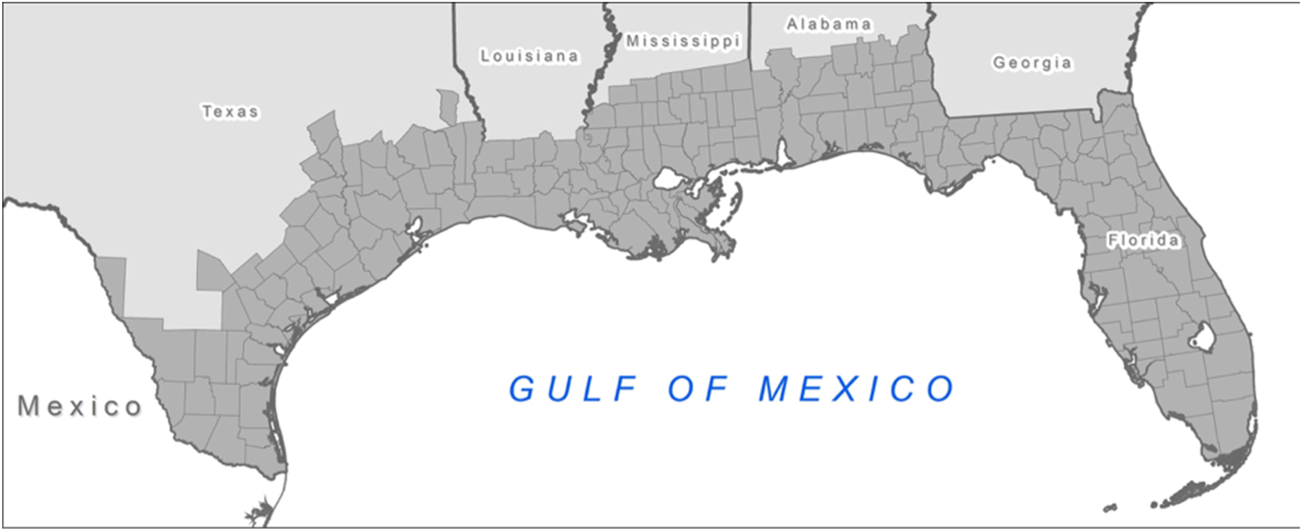
Map of Study Area
While previous studies have examined how flood risk affects housing prices and household preparedness, relatively little is known about how prospective homebuyers evaluate flood risk and mitigation options at the point of purchase, particularly in the context of varying risk representations. Most existing research relies on revealed preference data, which often lacks information on key home attributes or how buyers interpret risk. This paper addresses that gap by using a stated choice experiment to isolate and quantify homebuyer preferences for flood risk reduction, mitigation features, and alternative risk communication formats. The purpose of this research is to provide a clearer understanding of how risk perception, experience, and socioeconomic factors shape housing decisions in flood-prone regions.
In this paper we assess prospective homebuyer preferences for flood risk and mitigation features in US Gulf Coast states using choice experiments. Survey respondents are randomized to receive one of three flood risk representations: cumulative probability of flooding over a 30-year period, risk of flooding relative to neighbors, and average annual losses expected from flooding. In two choice experiments respondents choose which home they prefer to buy, with homes varying in price, size, interior quality, flood risk, and other flood related attributes. The first choice experiment assesses willingness to pay (WTP) to avoid flood risk and WTP for flood insurance. The second choice experiment assesses WTP for various home mitigation options. The findings indicate that preferences vary by risk representation and socio-demographics.
An online survey was administered to 1,040 respondents from April to June of 2021. The respondents were individuals 18 years of age or older who currently live in coastal counties in Alabama, Florida, Louisiana, Mississippi, and Texas (i.e., the study area), plan to move within the next five years within the study area, and plan to purchase a home when they move. A professional survey company, Qualtrics, assisted with sample recruitment, targeting a sample representative of the study area's age, race/ethnicity, and household income. Table 1 compares the sample socio-demographics to the population-weighted averages of the study area counties (obtained from the US Census Bureau's 2019 American Community Survey). The (un-weighted) survey sample is very close to representative on race/ethnicity and household income, though it proved difficult to recruit enough respondents over the age of 55 (possibly due to the online nature of the survey). Survey weights were developed and employed such that the estimation sample is exactly representative based on these socio-demographic characteristics.
Representativeness of Sample.
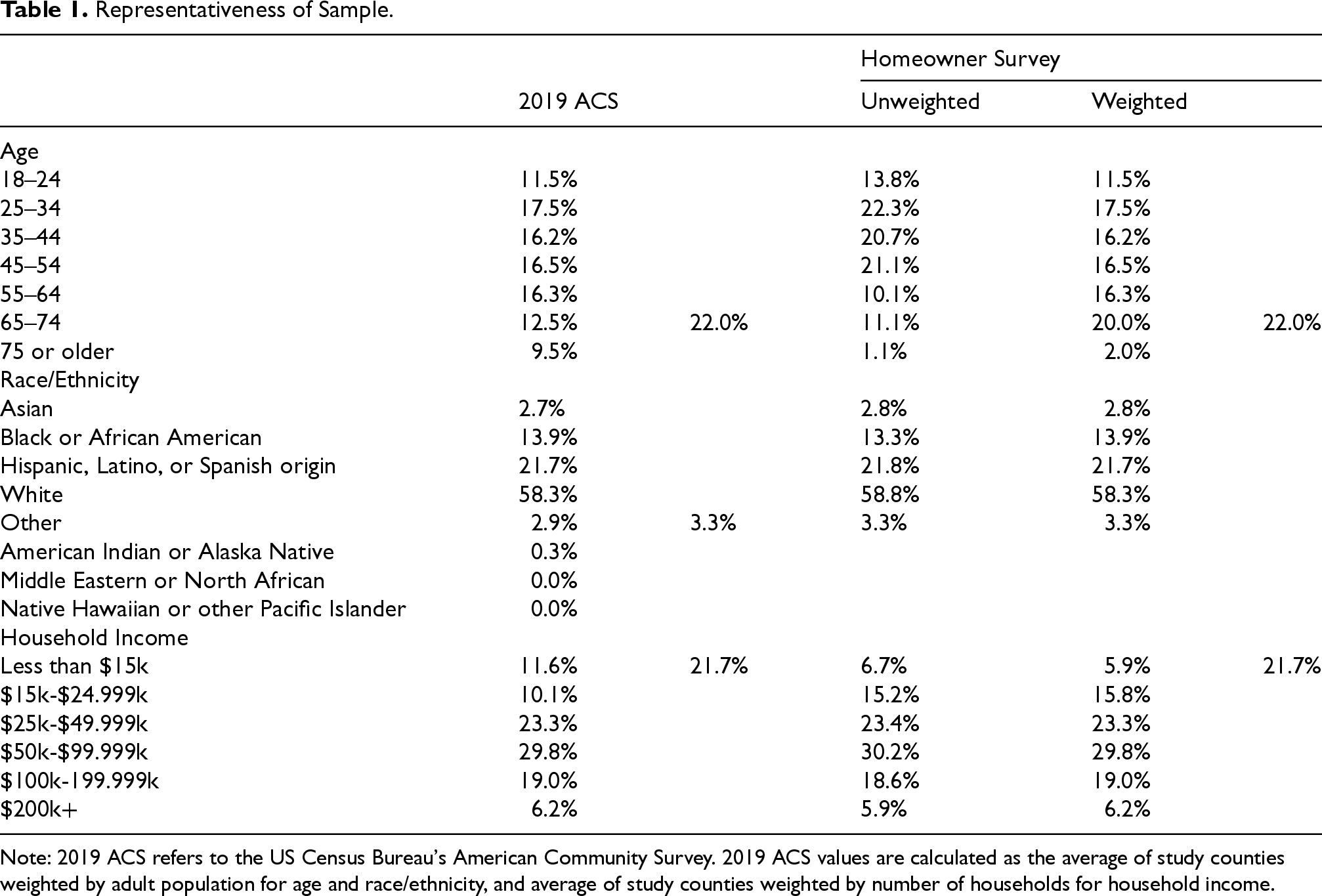
Representativeness of Sample.
Note: 2019 ACS refers to the US Census Bureau's American Community Survey. 2019 ACS values are calculated as the average of study counties weighted by adult population for age and race/ethnicity, and average of study counties weighted by number of households for household income.
The survey took 20 min to complete on average, with a median completion time of 16 min. The survey sought to minimize hypothetical bias and encourage incentive compatibility by stating, “Your response will help state and community leaders plan for future floods and understand the needs of households like yours.” 1 It began with screening questions to ensure a respondent was in the target population and then asked questions about mental health, past disaster exposure, and past home-buying experience, as a separate goal of the survey was to assess mental health impacts of floods and home-buying.
Next, respondents were randomly assigned to learn about flood risk via one of three different risk representations: cumulative risk, relative risk, or average annual losses expected from flooding. The cumulative risk representation presents flood risk in terms of probability of a home flooding in the next 1, 5, 15, and 30 years. The relative risk representation shows a home's risk of flooding compared to its neighbors (i.e., low, medium, and high risk). The average annual loss (AAL) is the net present value of average expected damage to a residential structure based on an underlying risk level. The three risk representations, as displayed in Table 2, are based on a common flood return period, which is a simple statistical tool taken from engineering practices, and is the most ubiquitous statistical concept used by hydrologists to describe risk of flooding (Volpi et al., 2015). In the US the most common representation of flood risk is the flood zones. The 100-year flood zone has a 100-year return period, and is an area where the probability of flooding in any given year is 1% (1/100 chance of flooding) (Zarekarizi et al., 2021). With information on the exposure and vulnerability of assets, flood risk can also be represented in terms of average annual losses, which provide an estimate of future flood-induced economic losses (Hsu et al., 2011; Orooji & Friedland, 2021; Rahim et al., 2022).
Equivalence of Risk Representations Across Flood Return Periods.
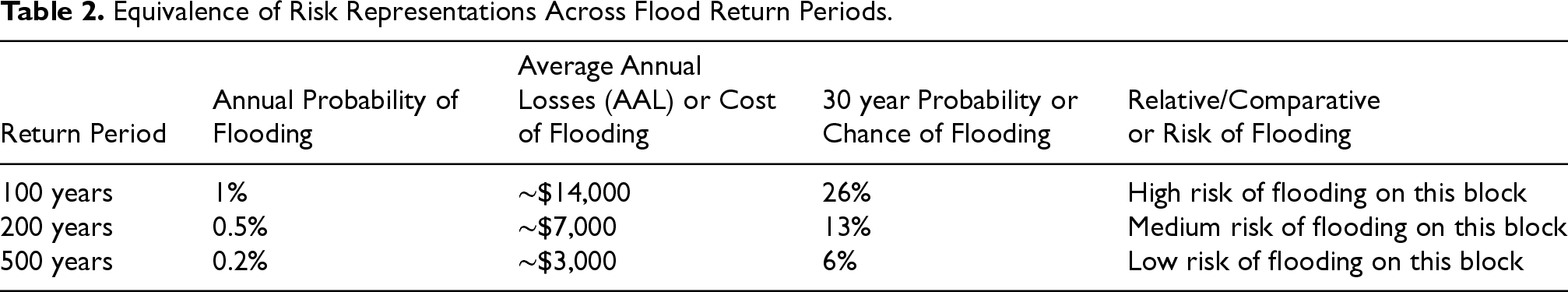
For timeframes longer than one year, we show total expected loss, which is the sum of AAL over years in the timeframe of a 30-year mortgage, a common financing arrangement in the US housing market. AAL values are obtained from Friedland (2021) and are based on square footage. Figure 2 shows images associated with each of the three treatments. These images were shown to respondents in addition to descriptive text, followed by two questions to assess comprehension of these representations.
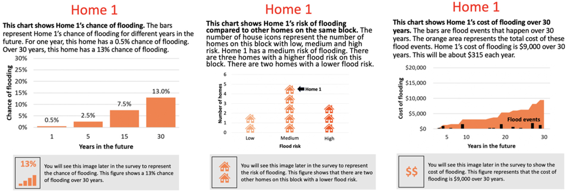
Flood Risk Portrayals
Next, respondents participated in two different choice experiments followed by several follow up and attitudinal questions. In each choice experiment, respondents answered three choice questions. In each question, respondents were shown two different homes with differing attributes and were told, “Out of the following two homes, please choose the home that you would be more likely to buy, assuming all the other features of the homes are the same.” They could also choose to buy neither home. Attributes in the first choice experiment include home price, size (square footage), interior quality, flood risk, and flood insurance. Since only a limited number of attributes could be included, size and interior quality were selected for the non-flood-based attributes because size can be a proxy for other important home factors (e.g., number of bedrooms and bathrooms) and interior quality is a rough measure of how “nice” a home is. Furthermore, prior literature involving choice experiments and home choice has shown the importance of these attributes (e.g., Bullock et al., 2011; Azimi & Asgary, 2013).
In addition to the aforementioned attributes, the second choice experiment also included mitigation attributes: elevated home, flood resistant floors, and/or flood resistant walls/ceilings. Figures 3 and 4 show example choice sets from the first and second choice experiments, respectively. Note that flood risk was represented according to treatment and that these three representations were based on the same underlying flood risk levels (with low, medium, and high risk representing 500-year, 200-year, and 100-year flood return periods).
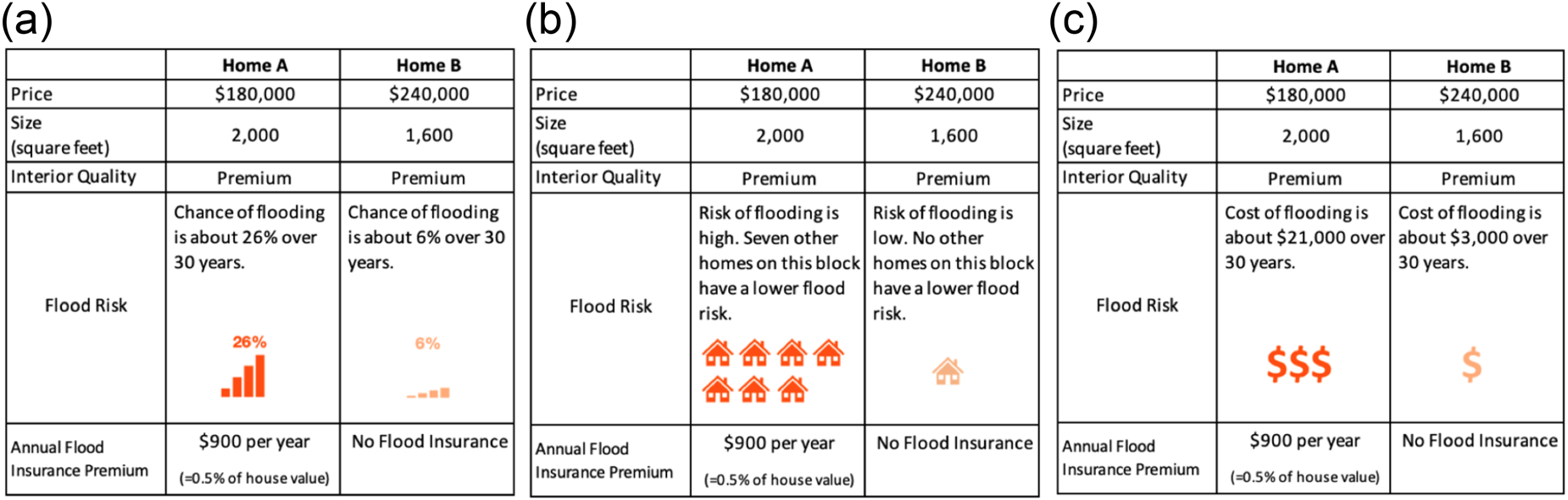
Sample Choice Set from First Choice Experiment
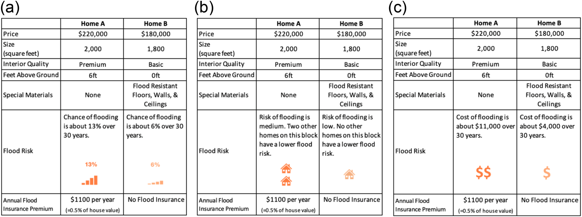
Sample Choice Set from the Second Choice Experiment
Prior to completing the choice experiments, each of the attributes was explained to the respondent. For example, the respondent was told “Basic interior means floors, cabinets, counters, and appliances are made of standard quality and ordinary materials. Basic interiors may include cheaper carpet and vinyl floors, laminate countertops, and lower-end appliances. Premium quality interiors are made of higher quality materials that are more durable. Premium interiors may include hardwood, tile, or better carpet floors, quartz or granite countertops, and higher-end appliances.” Each attribute description was accompanied by relevant photographs. See the full survey instrument in the Appendix for more details. Table 3 shows attributes and attribute levels used in the choice experiment.
Attribute Levels.
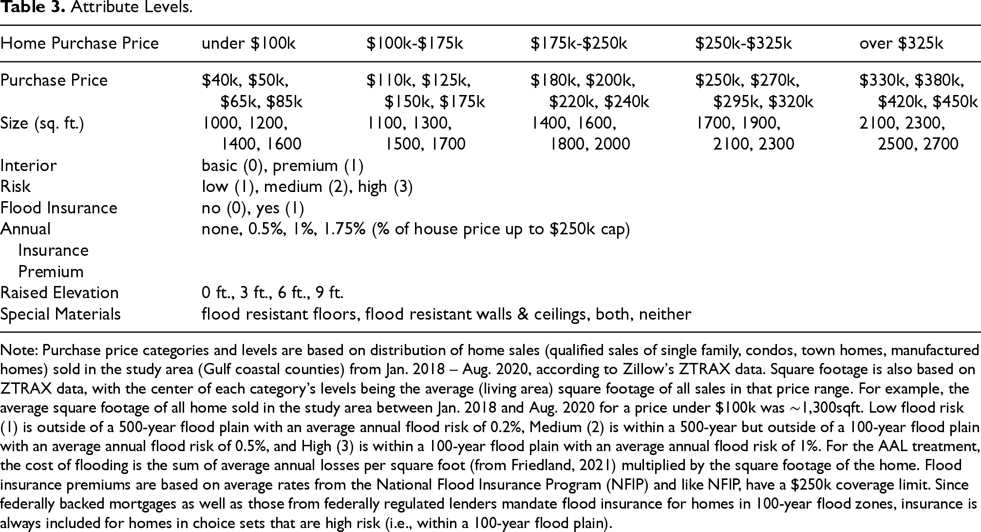
Note: Purchase price categories and levels are based on distribution of home sales (qualified sales of single family, condos, town homes, manufactured homes) sold in the study area (Gulf coastal counties) from Jan. 2018 – Aug. 2020, according to Zillow's ZTRAX data. Square footage is also based on ZTRAX data, with the center of each category's levels being the average (living area) square footage of all sales in that price range. For example, the average square footage of all home sold in the study area between Jan. 2018 and Aug. 2020 for a price under $100k was ∼1,300sqft. Low flood risk (1) is outside of a 500-year flood plain with an average annual flood risk of 0.2%, Medium (2) is within a 500-year but outside of a 100-year flood plain with an average annual flood risk of 0.5%, and High (3) is within a 100-year flood plain with an average annual flood risk of 1%. For the AAL treatment, the cost of flooding is the sum of average annual losses per square foot (from Friedland, 2021) multiplied by the square footage of the home. Flood insurance premiums are based on average rates from the National Flood Insurance Program (NFIP) and like NFIP, have a $250k coverage limit. Since federally backed mortgages as well as those from federally regulated lenders mandate flood insurance for homes in 100-year flood zones, insurance is always included for homes in choice sets that are high risk (i.e., within a 100-year flood plain).
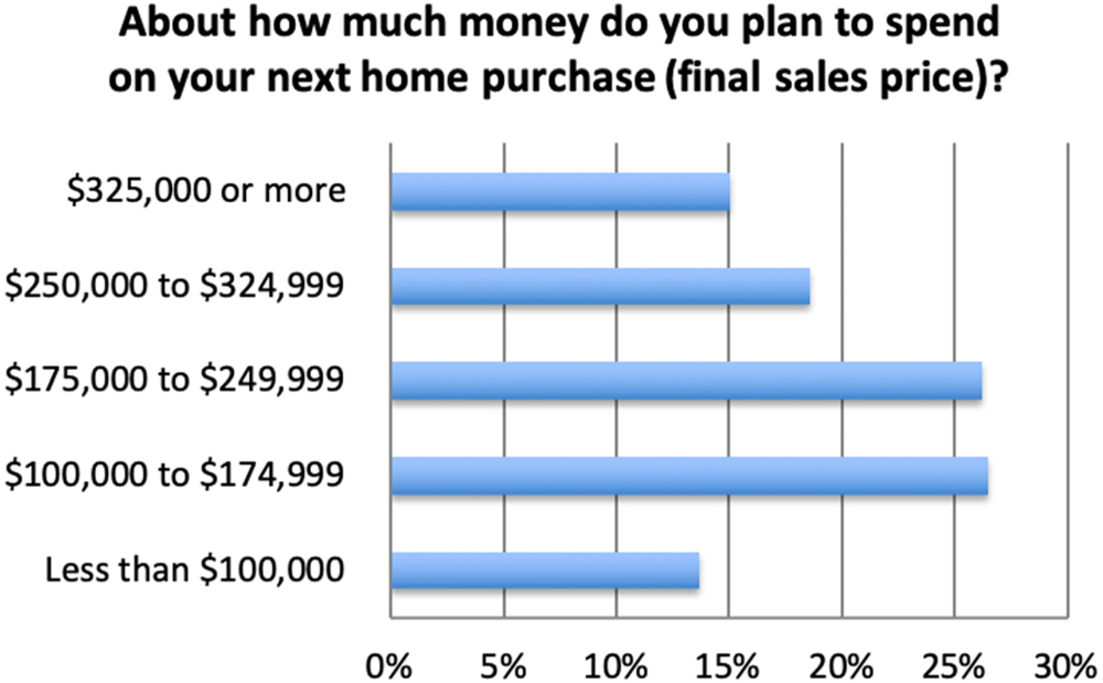
To make the choices more realistic, price levels were a function of the respondent's answer to the earlier question, “About how much money do you plan to spend on your next home purchase (final sales price)?” Respondents chose one of the five categories represented by the columns in Table 3. For example, respondents who indicated they would spend a maximum of $175k-$250k on their next home purchase would only see homes that cost $180k, $200k, $220k, or $240k. Square footage also scaled with home price. Each respondent was shown 3 choice sets out of a pool of 12 for each the first and second choice experiments. Figure 5 shows the percent of respondents who chose each home price category, and Figure 6 shows the survey logic that determined from which pool the choice sets were selected.
House Price Categories.
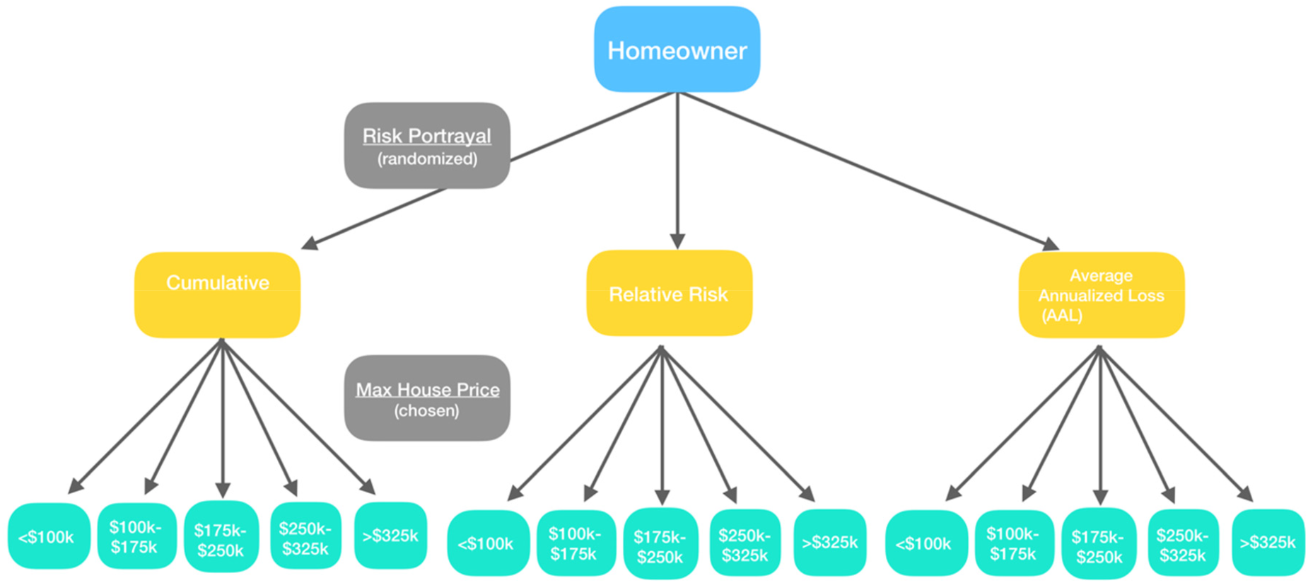
Logic Tree Determining Choice Set Pool.
To create the choice set pools, a separate choice experiment design was created for each of the five maximum home price bins using NGENE software. The experimental designs for the first and second choice experiment were based on the following utility functions, respectively:


We used an algorithm that sought to minimize the variance-covariance estimator of the vector of the coefficients from the utility function (Equations 1 and 2). This results in a design that maximizes the information gained from the choice experiment. Specifically, the algorithm varies alternatives within choice sets and choice sets within an experimental design to minimize the D-error, or the determinant of the asymptotic variance-covariance matrix. To further improve the efficiency of the experimental design, we specified Bayesian priors to indicate that
To determine the minimum sample size needed for reliable estimation of main effects in our discrete choice experiment, we follow the rule-of-thumb developed by Orme (1998, 2006). This guideline recommends a sample size of at least
We model the probability of choosing a home as a function of its attributes. The probability of a respondent choosing home is the probability that the utility from choosing home i is greater than the utility of choosing any other home:


If we assume that the error terms are independently distributed Type-I extreme value errors, we can model the probability of choosing home i as a conditional logit:

Once the coefficients from Equations 1 and 2 have been estimated, we calculate willingness to pay (WTP) for a 1-unit change in an attribute x as
To allow for heterogeneous preferences, we estimate a mixed logit rather than a conditional logit when we have enough statistical power. The mixed logit relaxes the independence of irrelevant alternatives property of the conditional logit and allows coefficients to be random parameters with normal distributions, rather than fixed parameters (Train, 1998). In the mixed logit the probability of choosing home i is:

Our approach aligns with applications of mixed logit models in environmental and housing economics. Prior research using these models includes Train (2009), Hensher and Greene (2003), and more recent applications in climate risk valuation (e.g., Entorf & Jensen, 2020; Kousky, 2011).
3.1 Caveats and Limitations
One limitation of our modeling approach is that the conditional logit estimates rely on the Independence of Irrelevant Alternatives (IIA) assumption, which may not fully capture complex substitution patterns across home alternatives. While we address this concern by also estimating mixed logit models—which allow for random coefficients and correlated errors—conditional logit results are still presented in some specifications for clarity and comparability. Future work could further explore flexible choice models, such as nested or latent class logit, to validate and extend these findings.
Our utility specification assumes a linear-in-parameters form, which implies constant marginal utilities for all attributes. While this is common in discrete choice modeling and facilitates estimation and interpretation, it may oversimplify preferences that are inherently non-linear—such as price sensitivity or risk aversion. Future work could explore non-linear specifications or transformations of key attributes to better capture these dynamics.
Furthermore, our models assume additive separability of utility across attributes, meaning that the marginal utility of one attribute does not depend on the levels of others. While this simplifies estimation and interpretation, it may limit the model's ability to capture interactions between home features—such as complementarities between mitigation measures and risk levels. Future research could explore interaction terms or more flexible utility forms to capture such interdependencies more explicitly.
In our mixed logit models, we assume normally distributed random coefficients to capture heterogeneity in preferences. While this allows for both positive and negative valuations—appropriate in cases like flood insurance, where some respondents may have aversion—normality can produce implausible tails, especially for price sensitivity. Although we chose not to model price as a random parameter due to insignificant variation and for ease of WTP estimation, this limits our ability to fully enforce monotonicity. Future work could adopt alternative distributions (e.g., log-normal) or estimate models in WTP space to better constrain parameter signs and improve the realism of preference distributions.
In some subgroup analyses—particularly for respondents in the highest intended home price category—our models exhibited convergence issues and extremely large standard errors for certain coefficients. These patterns suggest a lack of identifying variation and potential overfitting due to small sample size and weaker budget constraints in this group. To preserve model stability and interpretability, we exclude this tier from our preferred specifications. Nonetheless, these estimation challenges highlight the difficulty of modeling high-end segments in stated choice studies and the need for caution in interpreting subgroup-specific results with limited observations.
Our mixed logit models are estimated in panel form, accounting for within-respondent correlation by treating each respondent's set of choices as a panel and specifying random coefficients. While this captures unobserved preference heterogeneity and serial dependence across choices, future work could explore alternative modeling frameworks—such as latent class or hierarchical Bayes approaches—to further assess within-subject structure and preference segmentation.
Several additional limitations should be noted. First, although our use of Bayesian priors helped improve experimental design efficiency, it may introduce a degree of confirmation bias. We mitigated this risk by using weak priors limited to directional assumptions (e.g., price < 0), and final estimates are derived from fully empirical data. Second, while we incorporate heterogeneity in price sensitivity using interactions with income and stated home price intentions, our approach does not directly estimate the marginal utility of income. Future work could use continuous income variables or estimate models in WTP space to more explicitly capture income effects. Third, we assume a 30-year stream of insurance payments discounted at 2% to calculate net present value for premiums. WTP estimates are sensitive to this assumption; we now acknowledge this as a modeling choice and encourage sensitivity checks in follow-up studies.
Additionally, price may be endogenous to unobserved home quality or location factors, which we cannot fully address in this experimental setting. Relatedly, our choice sets exclude salient neighborhood features such as school quality or commute time, which may be correlated with flood risk and could lead to omitted variable bias. Finally, our models assume continuous, compensatory trade-offs among attributes. However, some respondents may treat flood risk as a deal-breaker—suggesting lexicographic preferences that violate these assumptions. Testing for such behavior or incorporating non-compensatory models (e.g., elimination-by-aspects) could be valuable extensions. Despite these limitations, we believe our approach offers meaningful insights into flood risk preferences under realistic constraints.
4.1. Experiment 1: Risk Levels and Risk Representations
For the first choice experiment, we first estimate the conditional logit from Equation 5. Table 4 displays the results, with coefficients estimated as log-odds. For homes with insurance, the annual premium is combined with the home price. Specifically, to home price we add the net present value of a 30-year stream of insurance payments, assuming a 2% discount rate. 3
First Choice Experiment Conditional Logit Results.
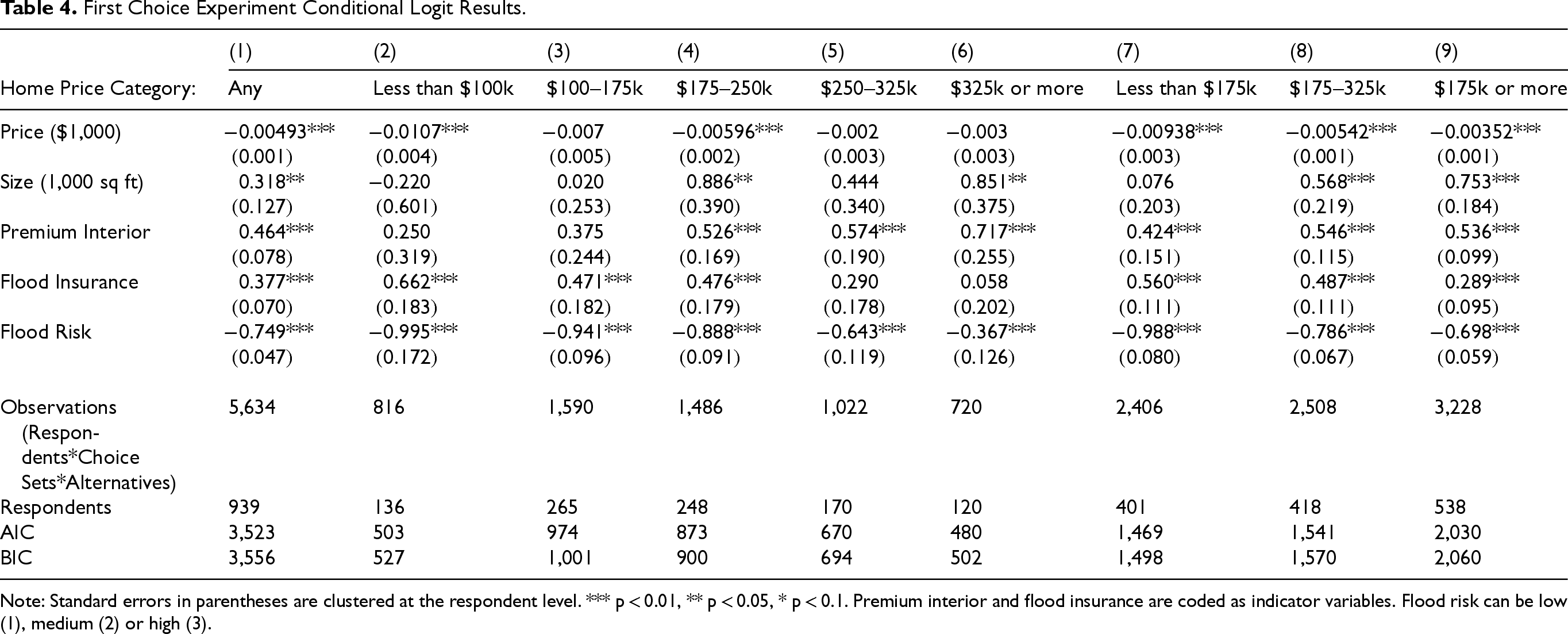
First Choice Experiment Conditional Logit Results.
Note: Standard errors in parentheses are clustered at the respondent level. *** p < 0.01, ** p < 0.05, * p < 0.1. Premium interior and flood insurance are coded as indicator variables. Flood risk can be low (1), medium (2) or high (3).
4.1.1. Willingness to pay for Home Flood Risk Attributes
The first column of Table 4 uses all respondents in the sample, while the remaining columns split the sample by maximum home price category. Generally, we expect that respondents planning to purchase less expensive homes will be more price-sensitive and might have different preferences for various attributes relative to those looking to purchase more expensive homes. Given the limited sample sizes in Columns 2–6, three of the price coefficients are not significant. However, respondents in the lowest home price category (Column 2) are roughly twice as price sensitive as those in the middle category (Column 4), as evidenced by the price coefficient being twice as large. In Columns 7–9 we combine home price categories to increase statistical power. Again, respondents in the higher home price categories (Columns 8–9) are less price-sensitive than those in the lower categories (Column 7), with smaller coefficients (in absolute value). The other attribute coefficients show that respondents have a positive preference for larger homes, homes with premium interiors, and homes with flood insurance, while they have a negative preference for homes with higher flood risk.
Throughout our analysis, data from the highest home price category ($325k or more) were somewhat troublesome. Fewer specifications achieved convergence, fewer results were statistically significant, and (for the mixed logit) some coefficient standard deviations were extremely large. In addition to this being the category with the fewest respondents, the models did not identify the upper limit to how much respondents are planning to spend on their next home purchase. However, the maximum price seen in any choice set is $450k. Thus, some of these respondents might be planning to spend a half a million dollars or more on their next home purchase. If so, not only would hypothetical bias be larger for these respondents, but the range of attributes (e.g., prices and sizes) might have reflected their real-world options poorly. If the cost of these homes was not an issue to these respondents, they could always choose the option with the attributes they care most about (e.g., largest or least risky) regardless of price, leading to very high willingness to pay for some attributes. As such, going forward, our preferred specifications are those that combine the first and second two house price categories (less than $175 and $175 to 325k) and omit the highest price category from analysis. Doing so also always results in better model fit (i.e., lower Akaike and Bayes information criteria, or AIC and BIC) relative to combining the three top categories ($175k or more).
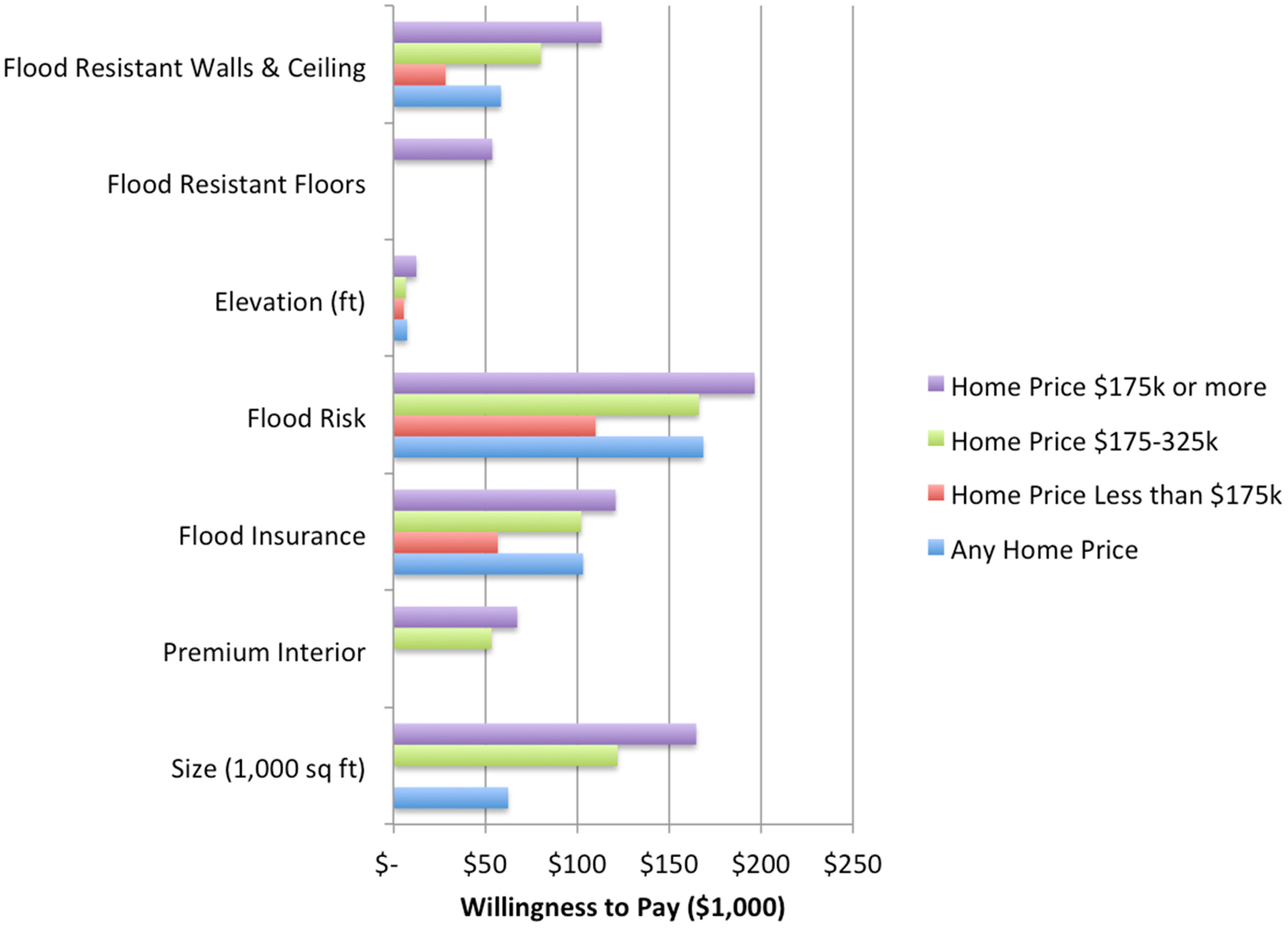
Willingness to pay (WTP) for a marginal increase in an attribute can be found by dividing an attribute's coefficient by the negative price coefficient. Figure 7 shows WTP values calculated from coefficients in Table 4 (note WTP is only calculated for statistically significant coefficients). 4 For flood risk, we multiply by negative one, such that values reflect WTP for a 1-unit decrease in flood risk (i.e., to change from high to medium, or medium to low risk). For all attributes, WTP scales with home price category (e.g., respondents planning to purchase lower price homes have lower WTP for size, premium interiors, flood risk, and flood insurance). Respondents are willing to pay between $65–214k per 1,000 square foot increase in home size and $45–152k for a premium (versus basic) interior. Respondents are willing to pay between $60–90k more for a home with flood insurance (versus without) and $105-$198k for a 1-unit reduction in flood risk. 5 Recall, a 1-unit reduction in flood risk means going from a high risk 100-year return period (annual probability of 1%), to a medium risk 200-year return period (annual flood probability of 0.5%), or from the latter to a low risk or 500-year flood return period (with an annual flood probability of 0.2%). Thus, a 1-unit reduction in risk roughly halves the annual probability of severe flooding.
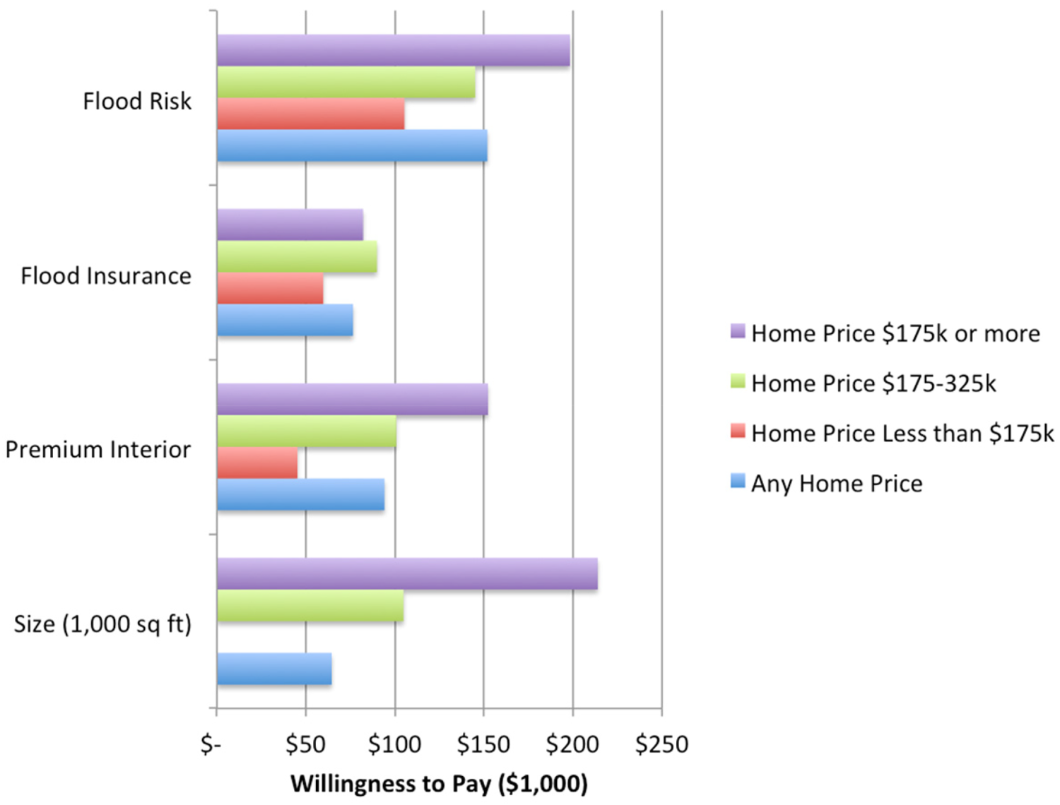
First Choice Experiment, WTP for Attributes based on Table 3.
4.1.2. Heterogeneous Preferences for Flood Insurance and Risk Reduction
To better explore preference heterogeneity, we next estimate a mixed logit using the data from the first choice experiment. The mixed logit allows specified coefficients to be random, with an estimated mean and standard deviation, rather than fixed. Because it is more computationally intensive than the conditional logit, we were unable to specify all coefficients as random parameters. When we attempted to specify the price coefficients as random parameters, their standard deviations were usually not significant, suggesting that allowing for different price coefficients across the home price categories sufficiently reflects heterogeneity in price sensitivity. Our preferred estimates specify flood insurance and risk as random parameters, both because these are the coefficients of most interest to our analysis, and because they consistently showed evidence of heterogeneous preferences (with significant estimated standard deviations). We do not specify price coefficients as random, as the interactions with income range already introduce preference heterogeneity to this attribute. Table 5 shows the results. Our preferred specification is Column 2, which interacts price with our preferred home price categories.
First Choice Experiment Mixed Logit Results.
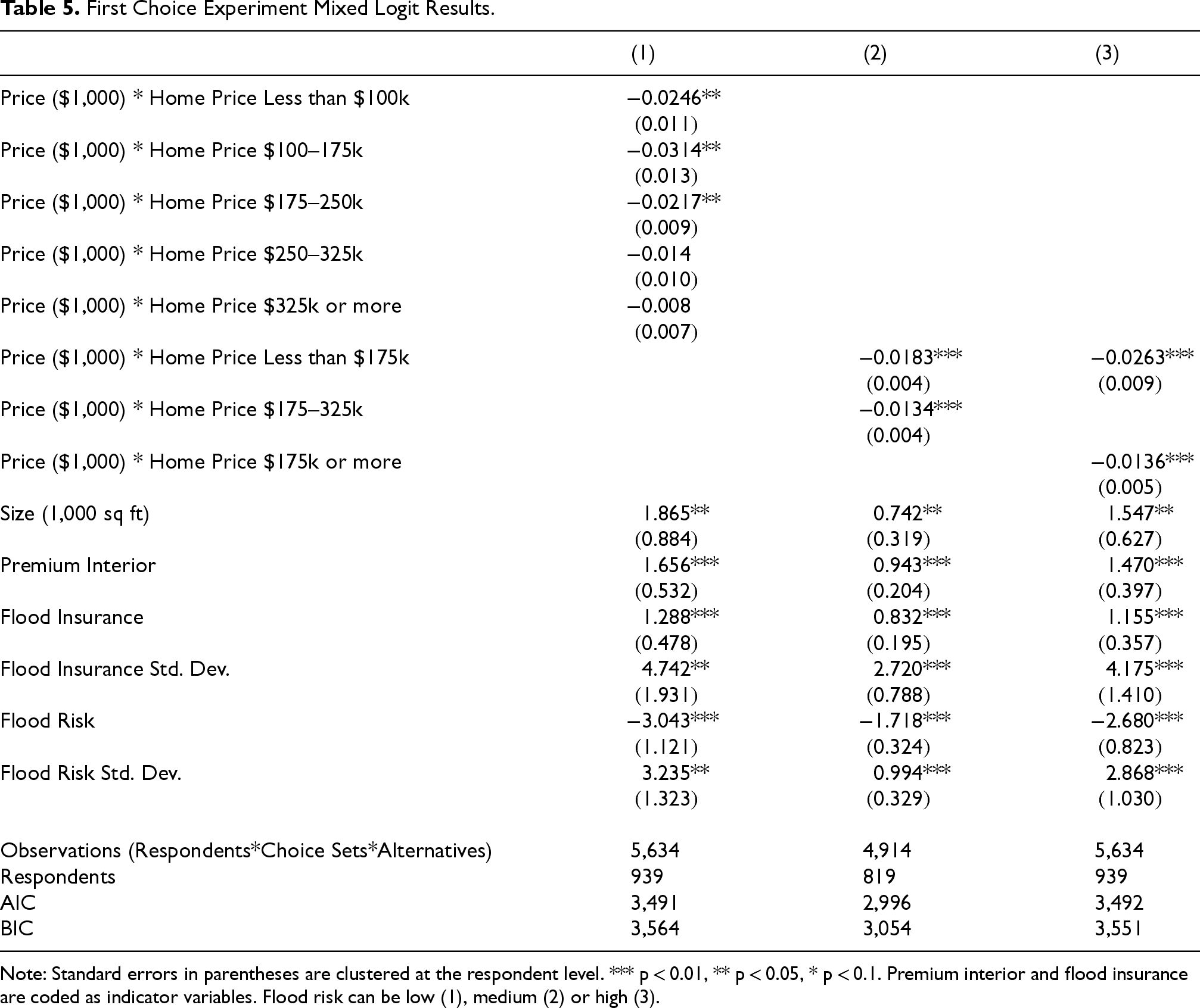
Note: Standard errors in parentheses are clustered at the respondent level. *** p < 0.01, ** p < 0.05, * p < 0.1. Premium interior and flood insurance are coded as indicator variables. Flood risk can be low (1), medium (2) or high (3).
To evaluate WTP for flood insurance and flood risk reduction based on the results in Table 5, we first estimate the elements in the coefficient covariance matrix. Then we calculate individual level parameters according to Revelt and Train (2000). Finally, we calculate the mean and standard deviation of the parameter distributions. Figure 8 shows kernel density estimates of the distribution of WTP for flood insurance and flood risk reduction for each home price category. Note that having estimated the coefficient covariance matrix, the individual parameters account for correlation across parameters- i.e., that an individual respondent's preference for flood insurance is correlated with their flood risk preference. WTP for both flood insurance and flood risk reduction is higher for the respondents in the higher home price category. Standard deviations of WTP are also high, suggesting substantial preference heterogeneity, with some respondents willing to pay high amounts for these attributes, and others not willing to pay much. A substantial portion of respondents has negative WTP for flood insurance. This could be due to a perceived lack of trust in the insurance providers, a desire to avoid the administrative burden of dealing with insurance companies, and/or a preference to self-insure.
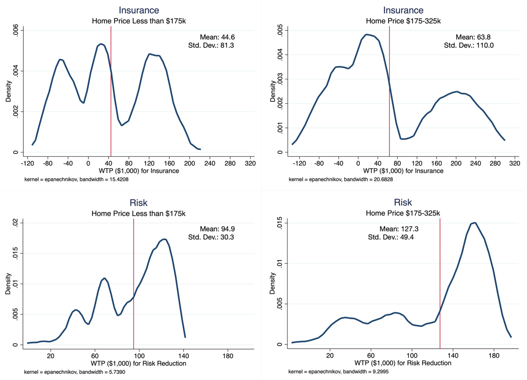
Kernel Density Estimates of Distribution of WTP for Flood Insurance and Flood Risk Reduction Based on Table 4 estimates.
To further explore heterogeneous flood risk preferences, we next interact flood risk with home price category, previous hazard experience, and the risk representation into which the respondent was randomized. This allows flood risk preference to vary along these three dimensions. Hazard experience is defined as the respondent indicating he or she has been displaced or lost their home due to a natural disaster. Table 6 displays the results. Figures 9–11 display the kernel density estimates of WTP distributions. In all cases, WTP is higher for respondents planning to purchase more expensive homes, due to their lower price sensitivity (smaller price coefficient in absolute value). Figure 9 shows that in addition to having a lower WTP for a 1-unit flood risk reduction ($103k versus $127k on average), those planning to purchase less expensive homes also have a much tighter WTP distribution than those planning to purchase a more expensive home, with a standard deviation of $17.9k compared to $52.6k. Notably, however, the difference in mean WTP is driven by differing price sensitivities (i.e., price coefficients), not different average risk preferences. The risk-home price interaction coefficients in column 1 of Table 6 show that respondents planning to buy lower priced homes do not have significantly different flood risk preferences than those planning to buy higher priced homes. Figure 10 shows that for both home price categories, home buyers with hazard-related displacement or home loss experience are willing to pay roughly $50–70k more for a 1-unit risk reduction, suggesting their prior experience has made them more sensitive to flood risk.
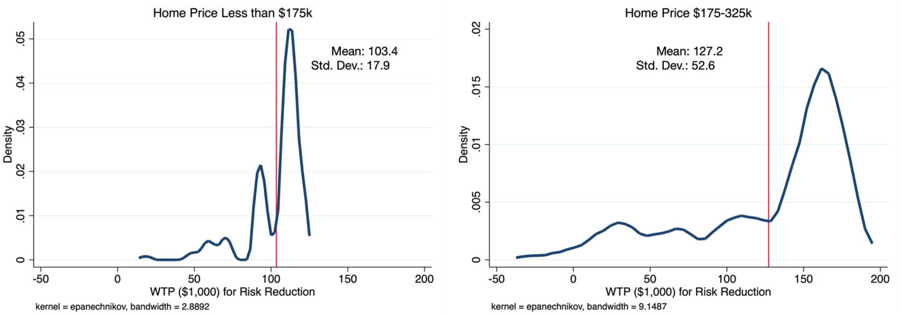
Heterogeneity in WTP for Flood Risk Reduction by Home Price Category Based on Table 6 estimates.
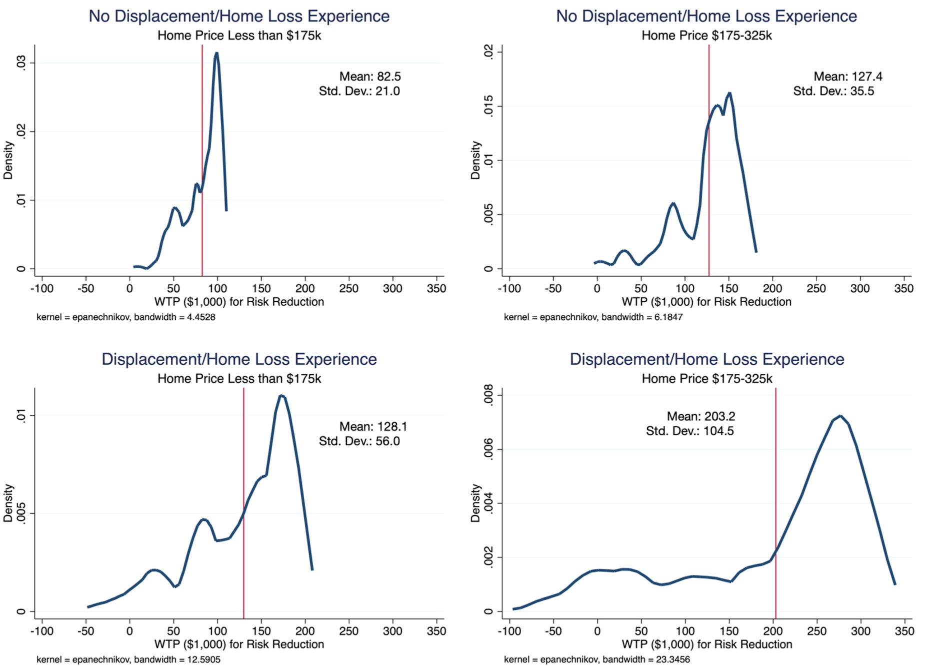
Heterogeneity in WTP for Flood Risk Reduction Hazard Experience Based on Table 6 estimates.
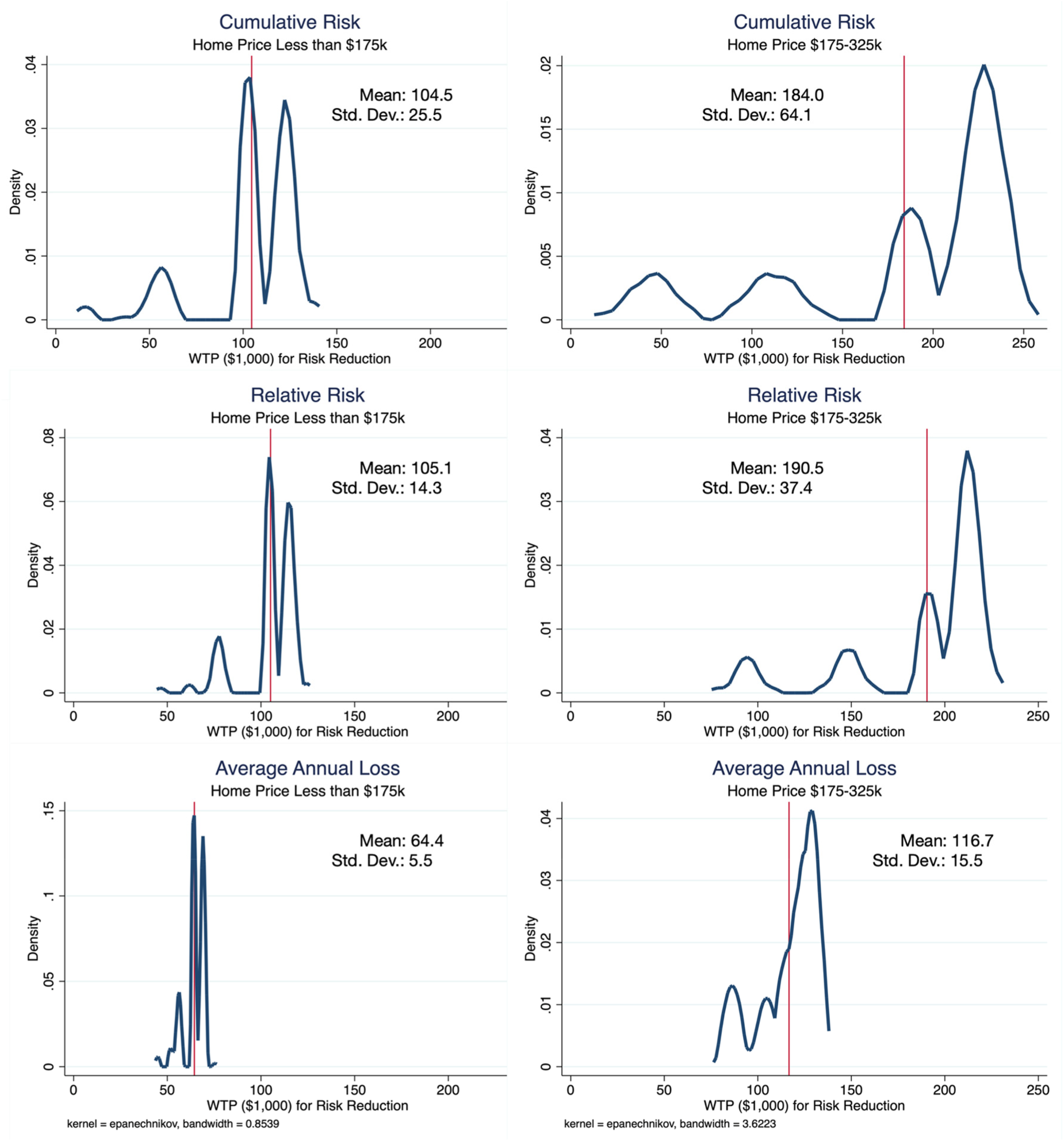
Heterogeneity in WTP for Flood Risk Reduction by Risk Portrayal Based on Table 6 estimates.
First Choice Experiment Mixed Logit Results with Flood Risk Interactions.
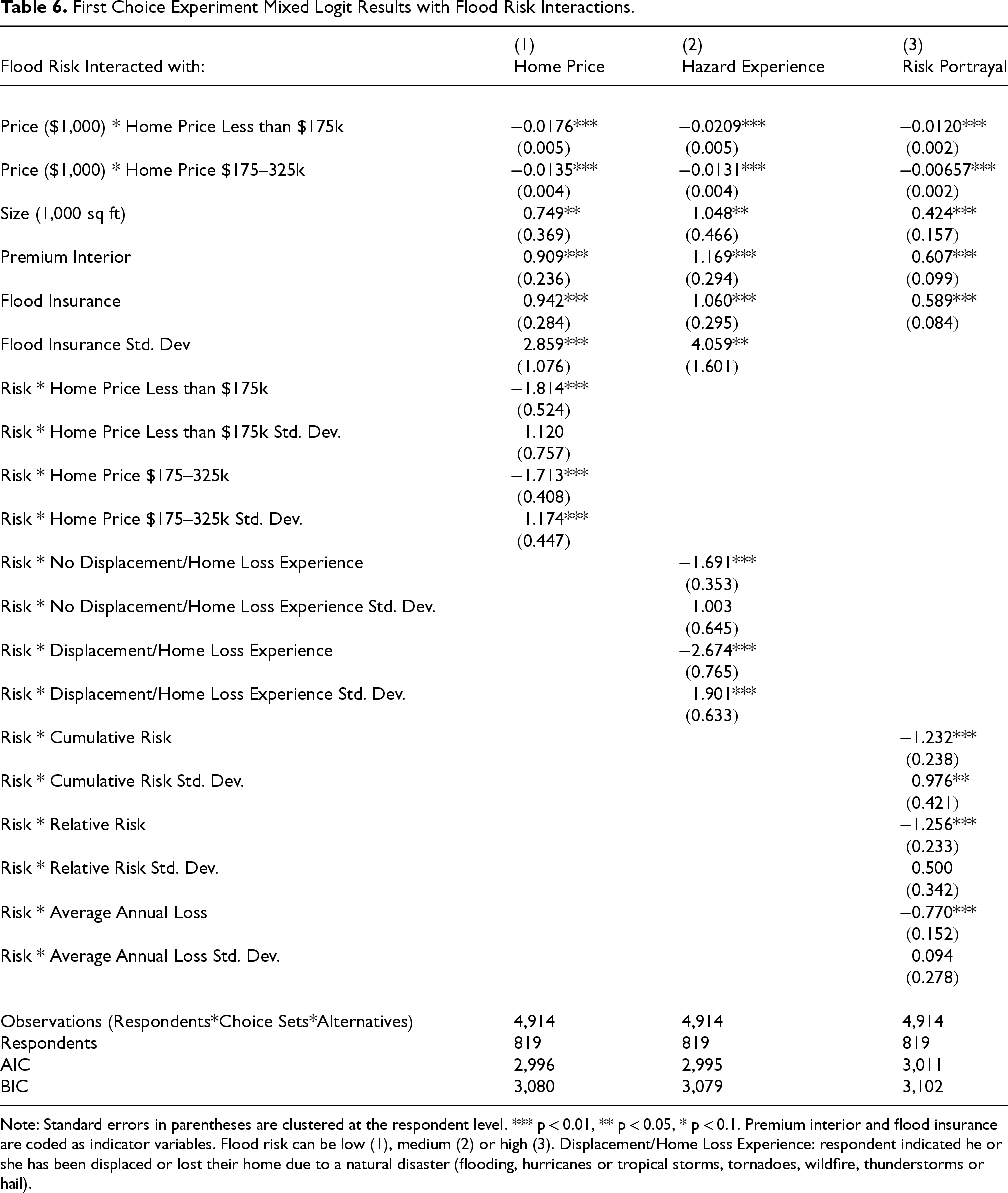
Note: Standard errors in parentheses are clustered at the respondent level. *** p < 0.01, ** p < 0.05, * p < 0.1. Premium interior and flood insurance are coded as indicator variables. Flood risk can be low (1), medium (2) or high (3). Displacement/Home Loss Experience: respondent indicated he or she has been displaced or lost their home due to a natural disaster (flooding, hurricanes or tropical storms, tornadoes, wildfire, thunderstorms or hail).
Figure 11 shows that WTP for risk reduction is similar for respondents who saw the cumulative and relative risk representations and substantially smaller for those who saw the average annual loss representation. This suggests that those seeing the non-monetary risk representations may actually overestimate the potential losses associated with a given risk level. The standard deviations of WTP for the average annual loss representation are smaller than those of the relative risk representation, which are in turn smaller than those of the cumulative risk representation. One explanation could be relative ease of understanding these different representations, with better general understanding or more familiarity (e.g., average annual loss) leading to smaller standard deviations, while more confusing or less familiar representations leading to larger standard deviations (e.g., cumulative risk).
The observed differences in willingness to pay across risk portrayals may also reflect underlying cognitive processing differences. For example, respondents shown average annual loss (a monetary framing) displayed both lower and more tightly clustered WTP values—consistent with dual-process theories of judgment and decision-making (Kahneman, 2011), where analytic (System 2) reasoning is more readily engaged by monetary values. In contrast, cumulative probabilities may prompt heuristic reasoning (System 1), increasing variability and potential overreaction. This interpretation aligns with research on risk perception that emphasizes the role of affective and intuitive processes in shaping risk judgments, particularly for low-probability, high-consequence events (Slovic, 1987; Slovic et al., 2004).
4.2. Experiment 2: Flood Mitigation Preferences
Next we focus on the second choice experiment, which is similar to the previous experiment, with the addition of flood mitigation attributes (i.e., elevation above ground level, flood resistant floors, walls, and ceilings). Given the increased complexity of this choice experiment and the larger number of coefficients to be estimated, we were generally unable to estimate the mixed logit model, as convergence was not achieved in most specifications. Table 7 shows the results of estimating a conditional logit for the second choice experiment, with the sample divided by home price category.
Second Choice Experiment Conditional Logit Results.
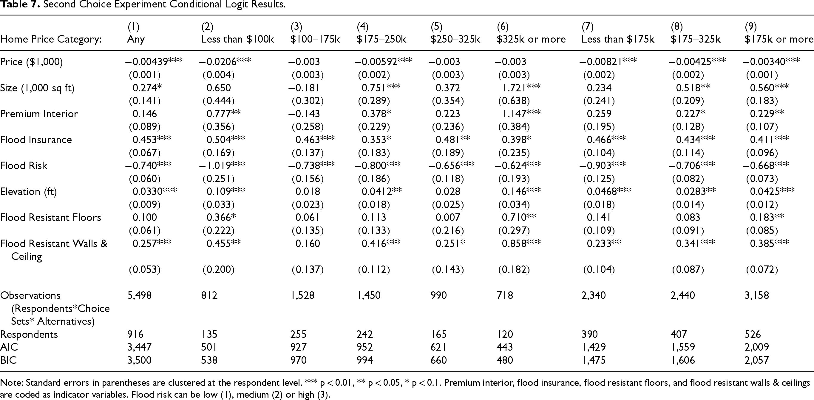
Note: Standard errors in parentheses are clustered at the respondent level. *** p < 0.01, ** p < 0.05, * p < 0.1. Premium interior, flood insurance, flood resistant floors, and flood resistant walls & ceilings are coded as indicator variables. Flood risk can be low (1), medium (2) or high (3).
Figure 12 displays the corresponding WTP estimates based on Table 7 (note WTP is only calculated for statistically significant coefficients). WTP for size, premium interior, flood insurance, and flood risk are similar to estimates from the first choice experiment. Respondents were willing to pay between $6–13k per additional foot of elevation above ground. This is on par with the national average cost of raising a foundation, which is $3–9k. 6 Respondents are willing to pay between $28–113k for flood resistant walls and ceilings. WTP is $54k for flood resistant floors in the only specification in which the coefficient is significant.
Second Choice Experiment, WTP for Attributes Based on Table 7.
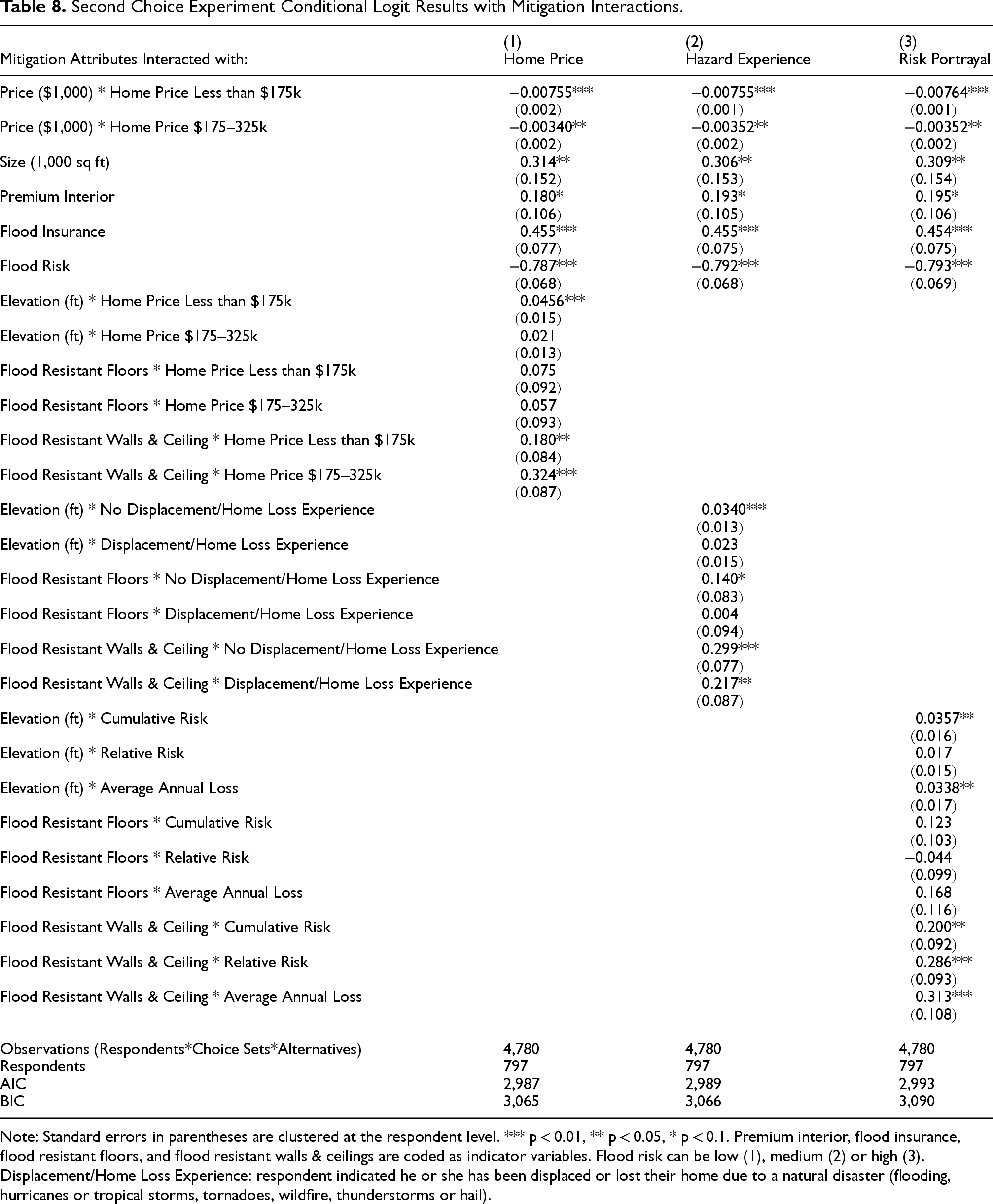
We next interact the three flood mitigation attributes with home price category, previous hazard experience, and risk representation to assess heterogeneous preferences along these three dimensions. Results are displayed in Table 8, with corresponding WTP calculations shown in Figure 13 (again, WTP is only calculated for statistically significant coefficients). There is no significant difference in WTP for elevation across risk representations. Although the point estimates suggest that respondents who have experienced hazard-related displacement or home loss are willing to pay somewhat less than those without such experience for flood resistant floors and walls, these differences are not statistically significant. Similarly, although WTP for flood resistant walls and ceilings appears to be highest for the average annual loss representations and lowest for the cumulative risk representations, these differences are not statistically significant. Hence, we are unable to identify factors associated with heterogeneous WTP for the mitigation attributes.
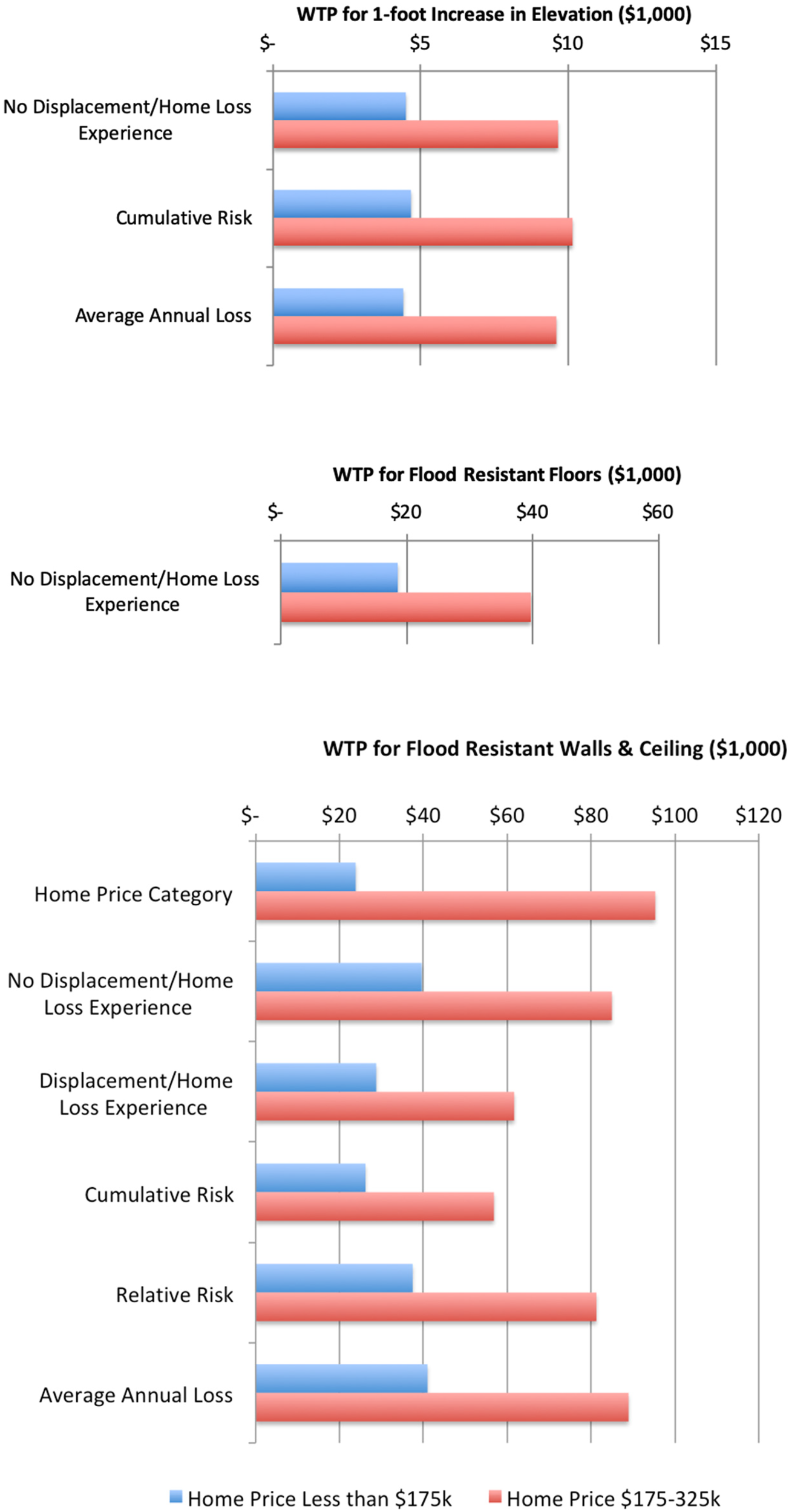
Heterogeneity in WTP for Flood Mitigation Attributes, Based on Table 8 estimates.
Second Choice Experiment Conditional Logit Results with Mitigation Interactions.
Note: Standard errors in parentheses are clustered at the respondent level. *** p < 0.01, ** p < 0.05, * p < 0.1. Premium interior, flood insurance, flood resistant floors, and flood resistant walls & ceilings are coded as indicator variables. Flood risk can be low (1), medium (2) or high (3). Displacement/Home Loss Experience: respondent indicated he or she has been displaced or lost their home due to a natural disaster (flooding, hurricanes or tropical storms, tornadoes, wildfire, thunderstorms or hail).
We find that in general, homebuyers in the Gulf Coast are responsive to flood risk and have a fairly high willingness to pay (WTP) for both flood insurance and a reduction in flood risk. On average, respondents are willing to pay $60–90k more for a home with flood insurance and willing to pay $100–150k to roughly halve their flood risk. However, a substantial number of respondents exhibited negative WTP for flood insurance, perhaps due to a distrust or dislike of insurance companies. WTP for flood risk reduction was generally higher than average projected flood losses (to a residential structure) over a 30-year period. There are several possible reasons for this. First, given the hypothetical nature of the choice experiments and the focus on flood risk, respondents may have over-reacted to the flood risk information. Second, respondents may not have fully understood the flood risk information in such a way as to translate it to projected losses, especially if they were shown cumulative rather than relative risk. Third, respondents may have been factoring in additional costs associated with flooding other than structural damage to the home. For example, they may have a higher WTP to avoid property damage, injury, and/or inconvenience (e.g., temporary or even permanent displacement, loss of work or school days) due to floods.
Though homebuyers planning to purchase lower priced homes have lower WTP on average, this is driven by higher price sensitivities rather than lower responsiveness to flood risk. Homebuyers who previously experienced displacement or home loss due to a natural disaster are willing to pay substantially more for flood risk reduction relative to those with no such experience ($128–203k versus $83–127k). We also find evidence that respondents who were shown flood risk in terms of average annual loss had a lower mean WTP for flood risk reduction with a smaller standard deviation. The smaller standard deviation is suggestive of lower uncertainty, indicating this risk representation may have been better understood by respondents.
We find that homeowners in the Gulf Coast are also generally willing to pay for flood mitigation measures. Average WTP for increased elevation is $6–13k, which is on par with actual costs. Most of our model specifications did not find a statistically significant WTP for flood resistant floors. However, we find an average WTP for flood resistant walls and ceilings of $28–113k. We do not find substantial heterogeneity in WTP for these measures by previous hazard experience or risk representation.
Our findings show that prospective homebuyers incorporate flood risk and mitigation into their decision-making, but their sensitivity depends on both experience and the framing of risk. The salience of monetary framing is consistent with dual-process models of cognition (Kahneman, 2011), while heterogeneity in response to probabilities supports Slovic's (1987) work on intuitive versus analytical processing. The large variation in WTP across respondents suggests the importance of tailoring flood risk communication and insurance options.
This study complements prior research by offering choice-based estimates for buyers rather than sellers, and by isolating responses to policy-relevant home attributes. Compared to past work using transaction data, our method allows us to estimate preferences for features like elevation and insurance cost that are typically unobserved in revealed preference settings. Our results also confirm and extend recent findings in the economics literature on floods (e.g., Bin & Landry, 2013; Gallagher & Hartley, 2017).
Conclusion
This study set out to answer four research questions: (1) Do homebuyers account for flood risk in purchase decisions? (2) How does risk framing affect perception? (3) What is the WTP for mitigation? and (4) How do demographics and experience shape preferences? Our results show strong evidence 1) that flood risk and mitigation affect homebuyer preferences, 2) that framing matters significantly, 3) that homebuyers have significant positive WTP for elevated structures and flood resistant walls and ceilings, and 4) that personal experience and income affect responsiveness. The use of a stated choice experiment enables us to explore these issues with a level of control and flexibility not available in market data.
The approach described in this paper forces individuals to choose in an environment where flood risk is one of the major attributes involved in the decision to buy a home. However, this is not the choice environment that homebuyers face in the real world. In the study area, the disclosure requirements for sellers in the housing market are minimal. The findings presented in this work suggest that information on flood or other disaster risk could play a larger role in home buying decisions if this information were provided to prospective buyers in a more prominent or easily understandable way. As flood risk increases in many parts of the United States, policy makers, insurers, and other interested actors in this space may consider policies or processes aimed to better inform homebuyers of their true flood risk.
Policy makers should recognize that how risk is communicated—probabilistically or monetarily—has material effects on homebuyer decision-making. Given that respondents preferred monetary framing and clearer information on insurance premiums, FEMA and state-level programs may benefit from simplifying flood risk tools and making insurance pricing more transparent. Our findings support the need for targeted subsidies or incentives for mitigation, particularly elevation, as well as ongoing education campaigns about residual risk outside of designated flood zones. This work also emphasizes the importance of incorporating behavioral insights—such as framing effects and risk heuristics—into climate resilience planning.
Supplemental Material
sj-docx-1-rda-10.1177_15697371251356795 - Supplemental material for Understanding Home Buyer Preferences for Flood Risk and Mitigation in a Flood-Prone Region
Supplemental material, sj-docx-1-rda-10.1177_15697371251356795 for Understanding Home Buyer Preferences for Flood Risk and Mitigation in a Flood-Prone Region by Tamara L. Sheldon, Michelle Miro and Sergio Alvarez in Violence Against Women
Footnotes
Ethical Considerations
This project received an exemption from the University of South Carolina's Institutional Review Board on 12/22/2020.
Consent to Participate
Survey participants provided written consent to participate.
Funding
This research is funded by the National Academy of Science Gulf Research Program Grant #18358A06-02.
Declaration of Conflicting Interests
The authors declared no potential conflicts of interest with respect to the research, authorship, and/or publication of this article.
Data Availability Statement
The data are available upon request from the authors.
Supplemental Material
Supplemental material for this article is available online.
Notes
References
Supplementary Material
Please find the following supplemental material available below.
For Open Access articles published under a Creative Commons License, all supplemental material carries the same license as the article it is associated with.
For non-Open Access articles published, all supplemental material carries a non-exclusive license, and permission requests for re-use of supplemental material or any part of supplemental material shall be sent directly to the copyright owner as specified in the copyright notice associated with the article.