Sage Journals: Discover world-class research

Abstract

The physical and morphological characteristics of wool and cashmere fibers exhibit notable similarities, making distinguishing them challenging. In this study, we propose a method based on a lightweight hybrid model called MobileViT, which combines a vision transformer and convolutional neural network, for the real-time identification of fiber categories. After training on a large sample dataset, the model was validated on a test set of 61,095 fiber images belonging to six categories; it took 26.2 s to achieve a recognition accuracy of 97.19%. This paper presents the first attempt to use a hybrid model of Transformer and Convolutional Neural Network (CNN) for the recognition of fiber images. Experimental results demonstrate that the model is capable of effectively extracting features from fibers, and it outperforms pure CNN models in terms of both speed and accuracy.

Keywords

MobileViT real-time identification fiber identification convolutional neural network vision transformer

Introduction

Cashmere is a high-end raw material commonly used in the textile and apparel industries because of its soft luster and excellent warmth retention. Wool resembles cashmere in terms of appearance, structural composition, and chemical properties. Therefore, cashmere is often blended with fibers such as wool. However, the price of cashmere is much higher than that of wool, and there has been a long-standing issue of wool being mixed with cashmere to counterfeit cashmere products as well as cashmere content being overstated in blended fabrics. Therefore, distinguishing cashmere and wool has always been a difficult problem in the field of fiber identification.

Researchers have proposed several methods for detecting cashmere fibers including microscopy,^1,2 DNA analysis,³ proteomic analysis,⁴ near-infrared spectroscopy (NIRS),⁵ and computer vision.^6,7 Microscopy and computer vision methods rely on the differences in the morphology of the fiber surface to identify fiber types. Microscopy involves manually observing the surface morphology of different types of fibers under an optical or electron scanning microscope to distinguish them, whereas computer vision methods store pre-captured images of fibers on a computer and use algorithmic models to extract visual features for fiber classification.

Proteomics analysis and NIRS are both used to identify fiber types through fiber composition analysis. In NIRS, a near-infrared spectrometer is primarily used to obtain the spectral signals of fiber mixtures, and then, mathematical models are used to calculate the proportions of different fiber types in the mixture. Proteomic analysis detects the amino acids of proteins in animal fibers to determine the content of the different fibers in mixtures of these fibers.

Among the aforementioned methods, the microscopic method is the oldest and most widely used in the field of fiber detection. Its popularity can be primarily attributed to its simple operation and mature detection standards. In comparison, NIRS and proteomic analysis use smaller sample sizes, and relevant standards for detection and analysis have not yet been established for these methods, raising the need for further studies with larger sample sizes.

In recent years, computer vision-based methods have become popular research topics in the field of fiber identification; they mainly extract features from the microscopic images of fibers. These methods can be classified into two categories: those that require manual feature specification and ones that perform feature extraction based on convolutional neural networks (CNNs).

Feature extraction methods such as scale-invariant feature transform and speeded-up robust features, which require manual specification, extract predetermined visual features from fiber images, such as the visual features of fiber surface textures or the measured values of fiber surface morphology indicators, such as fiber diameter and scale height. These features are then used to describe each fiber image, which is converted into a vector. Then, each vector is classified. Zhu et al.⁶ used the gray-level co-occurrence matrix method to extract texture features from fiber images and fused these features with the diameter value of the fiber, inputting them into a Fisher classifier for fiber classification. Similarly, Sun et al.⁷ used sparse dictionary learning to convert fiber images into vectors and then support vector machines for classification. The morphological characteristics of fibers, such as the density of surface scales, area height, thickness, and diameter, can also be used as fiber image features for fiber classification. For example, Xing et al.⁸ extracted the fiber diameter, scale height, and average scale area of cashmere and wool fibers and used Bayesian networks for fiber type determination.

Recently, with the rise of deep learning methods, CNN-based methods have become a particularly popular research topic. Unlike methods based on manually specified features, these methods use an end-to-end approach in which the fiber image is inputted into the convolutional network, and both feature extraction and classification are completed through a single network. Using the VGGNet model as a reference, Luo et al.⁹ established a CNN for classifying cashmere and wool fibers, achieving an accuracy of approximately 93%. Similarly, Cong et al.¹⁰ employed the Mask R-CNN model, inputting preprocessed fiber microscopic images into it for training and testing. Xing et al.¹¹ performed data augmentation on 65 fiber images and compared the accuracy of several classical CNNs for fiber recognition. The best performance was achieved when transfer learning had been applied to the VGG16 model. Zhu et al.¹² proposed an improved Xception network to identify cashmeres and wool fibers. Their method effectively mitigated the problems of insufficient feature representation and overfitting during network training.

In computer vision-based fiber detection methods, fiber samples are prepared using the standard microscopy method, in which microscopic images of fibers are manually observed, and the category of each fiber is directly determined. However, the discrimination process in computer vision-based methods is not based on human experience and manual observations. Instead, it involves first collecting fiber images and then using a fiber recognition model to determine the image category. A fiber recognition model typically uses supervised learning, in which the model is trained on a fiber image dataset with known categories. The training process involves learning the surface morphology pattern features of the fibers and saving them as model parameters. Finally, the model is used to predict the categories of the unknown fibers. Overall, computer vision-based methods, in which fiber category determination is performed through a computer model, can be considered an improvement over the manual microscopy method.

Recently, researchers have noted the excellent performance of the Vision Transformer (ViT) model in computer vision tasks. Inspired by this, we investigated the application of the ViT model to fiber identification, with the goal of developing a highly accurate and fast model with a low equipment demand that can make deploying detection terminals for automated fiber detection much easier. Our algorithm was built based on MobileViT, a lightweight model that exploits the potential for self-attention in its architecture. To the best of our knowledge, this is the first study that applies a hybrid model combining a CNN and ViT for fiber identification. The proposed model strongly outperformed existing fiber identification methods.

Method

We completed four main steps in the study. First, a dataset comprising over 60,000 optical microscopy (OM) images of six types of cashmere and wool fibers was prepared. Second, data augmentation techniques were applied to the training set images of the cashmere and wool fibers to mitigate the risk of overfitting. Third, the proposed MobileViT model was employed to train and validate the dataset, and the parameters were fine-tuned to optimize the performance of the model. Finally, alternative CNN models were trained and tested; and their accuracy, speed, and performance were compared with those of the MobileViT model for validation.

Convolutional Neural Network

A Convolutional Neural Network is a type of artificial neural network designed for processing structured grid data, such as images.^13,14 It is particularly adept at computer vision tasks. These networks typically include convolutional layers, pooling layers, and fully connected layers. Convolutional layers apply convolution operations to the input data, employing filters or kernels to extract local patterns and features. Pooling layers reduce the spatial dimensions of the data by down-sampling, preserving the most relevant information. The fully connected layers facilitate the learning of complex relationships by linking every neuron from one layer to the next. This structure enables CNNs to effectively learn and represent spatial hierarchies in the data. Their capacity for identifying hierarchical features and patterns in visual data has made them extremely effective in areas such as image recognition, object detection, and classification.

Vision transformer

A ViT is a deep-learning model specifically developed for computer vision applications. Unlike CNNs, which rely on convolutional layers to extract visual features from images, it employs a self-attention mechanism to capture the relationships and dependencies between various parts of an input image. This model has demonstrated a state-of-the-art performance on various benchmark datasets, demonstrating its ability to learn effective visual representations from large-scale image datasets.

Using the self-attention mechanism, the ViT network can demonstrate a remarkable proficiency in acquiring global visual representations. However, the abundance of weighting parameters in ViT-based models pose challenges for optimization. To successfully perform real-time fiber detection, a lightweight model called MobileViT, which combines the structure of a traditional CNN with a transformer-based framework, was adopted in this study. The fundamental concept of MobileViT involves leveraging transformers as convolutional layers to learn global representations. MobileViT incorporates the spatial inductive biases and robustness to data augmentation inherent in CNNs along with the input-adaptive weighting and global processing capabilities of ViTs, presenting a comprehensive solution for efficient and effective image analysis.¹⁵

MobileViT block

The MobileViT Block, which employs a transformer in a distinct manner, represents a crucial element within the MobileViT architecture. It attempts to effectively capture both the local and global information present in an input tensor while minimizing the number of parameters required. The structure of this block is shown in the upper part of Figure 1.

Figure 1.

MobileViT architecture,¹⁵ including the structure of the MobileViT block. Here, the term “Conv n×n” refers to a standard convolution operation with a n×n kernel, “MV2” represents the MobileNetv2 block, and the label “↓2” refers to the blocks responsible for down-sampling.

MobileViT block utilizes a n×n convolutional layer, followed by a 1 × 1 (or point-wise) convolutional layer, to process an input tensor (X) of shape H×W×C. The n×n convolutional layer captures local spatial information, whereas the point-wise convolution transforms the tensor into a higher dimensional (or d-dimensional where d exceeds C) space. This expansion is achieved by learning the linear combinations of the input channels, allowing the formation of richer representations. The resulting tensor X_L has a shape of H×W×d. Subsequently, in order to facilitate MobileViT block to learn global representations with spatial inductive bias, X_L is transformed into N nonoverlapping flattened patches, denoted as X_U, with a shape of N×P×d. Here, $N = \frac{W H}{P}$ is defined as the number of patches, with H and W representing the overall height and width of the input, respectively; and P is the product of two variables w and h, which represent the width and height of the patch, respectively.

Each patch of X_U is converted into a patch of X_G by applying transformers. The relationship between the patches can be represented as:

X_{G} (p) = T r a n s f o r m e r (X_{U} (p))

(1)

where $p \in {1, 2, \dots, P}$ , with $1 \leq p \leq P$ .

Contrasting with traditional ViTs being unable to capture the spatial arrangement information of pixels, MobileViT preserves both the patch order and the spatial order of pixels within each patch. Thus, X_F can be obtained by folding X_G. Subsequently, after applying a 1 × 1 convolution operation to X_F, it is combined with X through a concatenation operation, resulting in the projection of X_F onto a lower-dimensional space.

Therefore, X_U(p) captures local information by considering a neighboring n×n region using convolutions, whereas X_G(p) captures global information across P patches for the p-th location. This means that each pixel in X_G can contain information from all the pixels in X, enabling the comprehensive encoding of the entire input.

MobileNetV2 block

The main idea of MobileNetV2 (MV2) block is to introduce an inverted residual structure with linear bottleneck. Such a structure enhances the network’s ability to describe input information effectively. MV2 block takes a low-dimensional compressed representation as input, initially expanding it to a higher dimension, and subsequently filtering it through a depthwise convolution. Following this, features are projected back to a low-dimensional representation.¹⁶ The utilization of a linear activation function here is motivated by the potential information loss or degradation that may occur when transitioning from high dimensionality to low dimensionality using ReLU activation. Therefore, in the Projection layer of the MV2 block, a linear activation function is employed instead of ReLU to mitigate such issues. The structure of MV2 block is shown in Figure 2.

Figure 2.

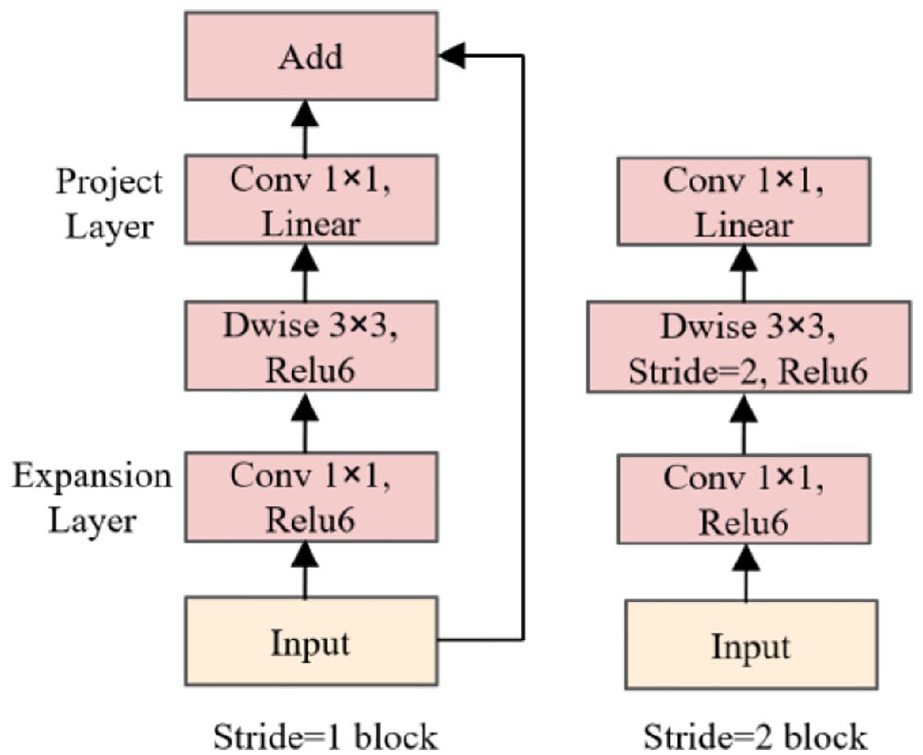
MV2 block.¹⁶

In the network design of MV2 block, in addition to continuing the use of the Depthwise Separable Convolution (Dwise) from MobileNetV1, the architecture incorporates both an Expansion layer and a Projection layer. As can be seen in Figure 2, the Expansion layer utilizes a 1 × 1 convolution to map the low-dimensional space to a higher-dimensional space, aiming to increase the number of channels (dimensionality expansion). On the other hand, the Projection layer, also employing a 1 × 1 convolution, seeks to map high-dimensional features to a lower-dimensional space, with the purpose of reducing the number of channels (dimensionality reduction). Depending on the value of the stride, the MV2 block defines two distinct blocks. The shortcut operation is employed only when the stride is set to 1, connecting the input and output features of the block (left part in Figure 2). Conversely, when the stride is set to 2, there is no utilization of a shortcut to connect the input and output features (right part in Figure 2).

MobileViT architecture

The architecture of the MobileViT is described in further detail below. The first layer of the architecture comprises a strided 3 × 3 standard convolution. This is followed by a sequence of MobileNetv2 (or MV2) and MobileViT blocks, as shown in the lower part of Figure 1. The convolutional module within the MobileViT block uses a value of n = 3, meaning that the convolution kernel is 3 × 3. The primary role of the MV2 blocks within the MobileViT network is to handle downsampling operations.

Uniqueness of MobileViT

Standard convolutions are understood as a sequence of three consecutive operations: unfolding, matrix multiplication, and folding. Both the MobileViT block and convolutions are similar in that they utilize similar building blocks. However, instead of relying on local processing through matrix multiplication, the MobileViT block employs deeper global processing using a stack of transformer layers. This substitution enables it to enhance its ability to capture global dependencies and generate more robust representations than those generated by traditional convolutions.

Contrasting with other models, MobileViT combines convolutions and transformers in a manner that endows the resulting MobileViT block with convolution-like properties while still facilitating global processing. This unique modeling approach enables the design of shallow and narrow MobileViT models that are lightweight in terms of computational requirements.

Each MobileViT model consists of three variants: small (S), extra-small (XS), and extra-extra-small (XXS), with each variant primarily differing in terms of the number of channels in the feature maps.

Experimental

Dataset

The dataset used in this study consisted of six types of fibers, comprising four types of cashmere and two types of wool: Mongolian brown cashmere, Chinese gray cashmere, Mongolian gray cashmere, Chinese white cashmere, Australian Merino wool, and Chinese indigenous wool, as shown in Figure 3. The samples were prepared by the Erdos Group in China.

Figure 3.

Microscopic images of six kinds of fiber: (a) Mongolian brown cashmere, (b) Chinese gray cashmere, (c) Mongolian gray cashmere, (d) Chinese white cashmere, (e) Australian merino wool, and (f) Chinese indigenous wool.

The fiber images were captured using optical microscopy at a magnification of 10 × 50. Noteworthily, each image contained a single fiber, and most of the fiber trunk was clearly visible. The total number of samples matched the total number of microscopy images. Consequently, the task of identifying animal fibers was transformed into fiber image classification.

In the prepared dataset, the number of samples for each type of fiber was approximately 10,000, resulting in 61,095 images for all six types. Specifically, there were 10,863, 10,181, 10,093, 10,013, 10,007, and 9938 fiber images for Mongolian brown cashmere, Chinese gray cashmere, Mongolian gray cashmere, Chinese white cashmere, Australian Merino wool, and Chinese indigenous wool, respectively.

In the preprocessing phase, all original sample images were resized to 256×256 pixels. To enhance the dataset, data augmentation techniques such as horizontal and vertical flipping of images were employed. This approach was specifically applied to the training set images of cashmere and wool fibers, aiming to reduce the risk of overfitting and improve the model’s generalization ability. These augmentation techniques not only diversify the training data but also simulate various orientations and perspectives, ensuring a more robust and effective training process.

To enhance the dependability of the training and validation processes of our proposed solution, we implemented a 10-fold cross-validation method. Regarding cross-validation, it facilitates the assessment of the performance of a model by dividing the available data into multiple subsets or folds.

Accordingly, the dataset was divided into two nonoverlapping subsets: training and test sets. To accomplish this, each type of fiber was randomly divided into 10 equal parts, with one part from each type of fiber taken to form a subset (fold). Then, one subset was selected as the test set, and the remaining nine parts in the dataset constituted the training set. This division was repeated ten times, and each time, the selected test set did not overlap. Figure 4 schematically represents the division of a dataset into subsets.

Figure 4.

Division of the 10-fold cross-validation dataset.

As shown in Figure 4, the dataset was divided into 10-folds using the aforementioned approach. Next, each fold was iterated and used as a test set while the model was trained on the remaining folds. For instance, in the first iteration, the model was trained on folds 1–9 and tested on fold 10. In the second iteration, it was trained on folds 1–8 and 10 and tested on fold 9. This process was repeated for all the folds. After training and testing the model on all the folds, its performance was assessed by calculating the average evaluation metric across all the iterations. This helped mitigate the bias introduced by the training-test split.

Experimental setup

Our experiment was performed on hardware with an AMD R7-4800HS CPU at 2.9 GHz, 16 GB of running memory, and an RTX 2060 GPU with 6 GB of memory. The initial weight values of the model were set using the pretrained weights obtained from training the model on the ImageNet dataset. These weights were used as a starting point for fine-tuning, allowing the model to leverage pre-existing knowledge to improve its performance in the task.

The hyperparameters were set after tuning the model. The batch size was set to 16, a stochastic gradient descent (SGD) optimization algorithm was applied during training, and the learning rate was initially set as 0.00625. This learning rate configuration followed a step-based learning rate scheduling strategy, in which the learning rate was updated every two epochs by multiplication by a factor of 0.973. The change in the learning rate during the training of the MobileViT model training is shown in Figure 5.

Figure 5.

Changes in the learning rate during the training process.

Regarding momentum, it is a technique in which a fraction of the previous update vector is added to the current update to accelerate SGD, thereby enabling faster convergence. The momentum value was set to 0.9, indicating that 90% of the previously updated direction had been incorporated into the current update; and the weight decay was set as 0.0001. Weight decay is a regularization technique that adds a penalty term to the loss function, encouraging the model to have smaller weights and reducing overfitting.

Evaluation metrics

We selected a diverse set of metrics to evaluate the performance of the proposed model. The metrics used in our evaluation were accuracy, precision, recall, and F1 score. These metrics are explained following the clarification of the concept of the confusion matrix below.

The confusion matrix provides a comprehensive breakdown of model predictions by comparing them with actual labels.¹⁷ This matrix includes the following components: true positives (TPs), true negatives (TNs), false positives (FPs), and false negatives (FNs). Analyzing the values in the confusion matrix can provide insight into the accuracy, precision, recall, and other relevant metrics of a model. Regarding TPs and TNs, they represent cases in which a model correctly predicts a positive and negative class, respectively, while FPs and FNs refer to cases in which a model incorrectly predicts a positive and negative class, respectively.

Accuracy represents the overall accuracy of model predictions across all classes. It is calculated as the ratio of the sum of TPs and TNs to the total number of instances in the dataset. The formula for accuracy is as follows:

Accuracy = \frac{T P + T N}{T P + T N + F P + F N}

(2)

Precision measures the accuracy of positive predictions made using a classification model. It focuses on the proportion of TP predictions to all the positive predictions, including both TPs and FPs. The formula for precision is as follows:

Precision = \frac{T P}{T P + F P}

(3)

Recall is a metric that measures the ability of a model to correctly identify the positive instances out of all the actual positive instances in the dataset. In other words, the recall quantifies the completeness of a model in identifying positive cases, with a higher recall value indicating that a model has a lower tendency to miss positive instances and a better ability to capture them. The formula for the recall is as follows:

Recall = \frac{T P}{T P + F N}

(4)

The F1 score is a commonly used metric derived from the confusion matrix that combines the precision and recall into a single value. It provides a balanced measure of the model performance, particularly in situations where there is an imbalance between classes. It balances the tradeoff between precision and recall and provides an overall assessment of the performance of a model. The formula for calculating the F1 score is as follows:

F 1 Score = 2 \frac{P r e c i s i o n \times R e c a l l}{P r e c i s i o n + R e c a l l}

(5)

Results

Training and testing

As mentioned previously, we employed a 10-fold cross-validation technique to train and assess the performance of the proposed method. Prior to training, data augmentation was performed on the dataset. The sample images in the training set were first randomly cropped to 224 × 224 images and then subjected to horizontal and vertical flipping. Finally, random rotation was applied to them.

Before being fed into the model for training, the samples in the training set were subjected to normalization, in which each channel of the image was subtracted from its corresponding mean and divided by its corresponding standard deviation. Specifically, the RGB value of each pixel was subtracted from [123.675, 116.28, 103.53] and divided by [58.395, 57.12, 57.375]. This normalization aimed to map the pixel values of the image to a range with a mean of zero and a standard deviation of one. This technique helped improve the stability and convergence speed of model training.

Before being fed into the model for validation, the sample images in the training set were subjected to center cropping, in which a square region was extracted from the center of each image. The size of each image was resized and cropped to 224×224 pixels. This ensured consistency in the dimensions of the cropped images, allowing seamless processing and evaluation.

In the experiment, three models – MobileViT_S, MobileViT_XS, and MobileViT_XXS – were trained and tested individually. Here, MobileViT_XXS is discussed as an example to describe the training process and the test results. Table 1 presents the values of the evaluation metrics for each fold in the 10-fold cross-validation experiment.

Table 1.

Ten-fold cross-validation results in terms of evaluation metrics.

Fold	Accuracy (%)	Precision (%)	Recall (%)	F1 Score (%)
1	97.28	97.27	97.26	97.26
2	97.48	97.46	97.46	96.46
3	97.25	97.23	97.23	97.23
4	96.81	96.81	96.78	96.79
5	97.15	97.14	97.13	97.13
6	97.82	97.8	97.81	97.8
7	97.71	97.69	97.69	97.69
8	96.69	96.68	96.66	96.67
9	96.79	96.79	96.77	96.77
10	96.92	96.92	96.90	96.90

Figure 6 illustrates the change curves of the training loss of the model during the first 10-fold experiment. The training loss clearly exhibited a decreasing trend, gradually converging as the number of epochs increased. At approximately 300 epochs, the loss stabilized.

Figure 6.

Changes in the accuracy for the training set during training.

Figure 7 illustrates the variation curve of the accuracy for the test set during the first fold of the 10-fold experiment. Before reaching 250 epochs, there was a substantial fluctuation in the values. However, after 300 epochs, the magnitude of the oscillation decreased significantly and gradually approached stability. In this experiment, the model achieved an accuracy of 97.28% on the test set. Owing to the similarity between the curves for the other evaluation metrics (precision, recall, F1 score, and accuracy), the corresponding line graphs have not been provided here.

Figure 7.

Changes in the accuracy for the test set during training.

The first three-fold confusion matrices for the identification of the six types of fibers in the test set are shown in Figure 8.

Figure 8.

Confusion matrices in the 10-fold cross-validation for (a) fold 1, (b) fold 2, and (c) fold 3.

After the 10-fold cross-validation experiment, the model achieved an average accuracy of 97.19% for the test set. The average precision, recall, and F1 score were 97.18%, 97.17%, and 97.07%, respectively.

In the experiment, c_brown, c_greycn, c_greymgl, c_white, w_mer, and w_indig represented the Mongolian brown cashmere, Chinese gray cashmere, Mongolian gray cashmere, Chinese white cashmere, Australian merino wool, and Chinese indigenous wool, respectively. The confusion matrix provided valuable insights into the classification process. In this matrix, the columns represent the predicted values for each class, the rows denote the actual classes of fibers, and the diagonal elements indicate the accurate identification count for each fiber class.

Consider the confusion matrix for fold 1, which is shown in Figure 8(a). Each cell in row 1 represents the number of Mongolian brown cashmere images predicted to belong to the various fiber classes. As shown in Figure 8(a), 1077 of the 1086 Mongolian brown cashmere images in the test set were predicted correctly, with two, three, and four predicted to be Chinese gray cashmeres, Chinese white cashmeres, and Australian Merino wool, respectively. Moreover, the identification accuracy of Australian Merino wool (row 5) was relatively high, and only three images were incorrectly predicted. In comparison, the identification accuracy for the other four types of fibers was low. Incorrect predictions were observed for 43 of the 1018 Chinese gray cashmeres, 37 of the 1009 Mongolian gray cashmeres, 37 of the 1001 Chinese white cashmeres, and 39 of the 993 Chinese indigenous wool samples.

Predicted probabilities of the inputted fiber images

Using the MobileViTXSS model, the model predictions for each sample were examined. The classification layer employed softmax regression to compute the probability value of the inputted fiber image for each category. The category associated with the highest probability value was selected as the predicted category for the fiber. Figure 9 shows the model prediction results for the two sample categories.

Figure 9.

Prediction results for (a) Mongolian brown cashmere and (b) Chinese gray cashmere.

Comparison of MobileViT and CNNs

In the experiment, the performance of the MobileViT was compared with that of the other CNNs on the same dataset of fiber images. Table 2 contains the number of parameters, test time and accuracy of these models, where the test time is the time for the model to run on the test set, which contains 6109 samples.

Table 2.

Comparison of the number of parameters, testing time, and accuracy on a 2060 GPU (6 GB VRAM) for various models.

Model	# Weights	Time	Accuracy (%)
ResNet18	11.7 M	37.2 s	97.08
ResNet50	25.6 M	39.8 s	96.33
ResNet101	44.5 M	49.2 s	96.08
SEResNet101	28.1 M	51.8 s	95.97
MobileNetV3_Small	2.9 M	26.0 s	97.10
MobileViT-XXS	1.3 M	26.2 s	97.19
MobileViT-XS	2.3 M	33.6 s	97.25
MobileViT-S	5.6 M	35.1 s	97.41

As shown in Table 2, the MobileViT series models had the fewest parameters, facilitating the deployment of detection systems on terminal devices. Both MobileViT_XXS and MobileNetV3_S required approximately 26 s for execution on the validation set, with MobileViT_XXS achieving a higher accuracy and having significantly fewer weights. The MobileViT_XXS model, which had fewer weights, took an additional 0.2 s to run compared to that taken by MobileNetV3_Small. This is because CNNs leverage the characteristics of the local receptive fields and shared weights to achieve efficient image feature extraction with fewer parameters. By contrast, ViT models utilize self-attention mechanisms to capture global relationships in images, requiring multiple attention computations on input sequences, leading to a higher computational complexity and runtime. In the fiber image recognition experiments conducted in this study, the hybrid MobileViT model, which combined CNNs and ViT, achieved detection with a fast speed and high accuracy. Additionally, MobileViT has fewer weights, making it more suitable for real-time fiber detection.

Comparison of the proposed method with other methods

Table 3 presents a comprehensive comparison of the proposed method with various existing techniques used for visual feature-based fiber identification. Table 3 also lists the number of sample categories, number of samples, methods for sample image collection, feature extraction methods, and the accuracy of each of these methods.

Table 3.

Comparison of the proposed method with other methods.

Method	Number of species	Number of samples	Sample collection methods	Feature	Accuracy (%)
Xing et al.¹⁸	3	150	OM	Texture feature	90.07
Tao et al.¹⁹	2	1000	OM	Morphology and texture	93.1
Xing et al.⁸	2	1000	OM	Morphological	94.2
Zhu et al.⁶	2	1200	SEM	Fiber diameter and texture	96.71
Wang and Jin²⁰	2	1980	OM	CNN	92.1
Luo et al.²¹	6	60,000	OM	CNN (Resnet18)	97.1
Yildiz²²	2	100	OM	CNN	98
Zhu et al.¹²	2	955	SEM	CNN (Improved Xception)	98.95
Xing et al.¹¹	4	65	OM	CNN (VGG16)	99.15
Ours	6	61,095	OM	MobileViT_XXS	97.19
Ours	6	61,095	OM	MobileViT_XS	97.25
Ours	6	61,095	OM	MobileViT_S	97.41

The results in the first four rows in Table 3 are based on manually extracted features. Among these, the method used by Zhu, which utilized 1200 fiber images, achieved the highest accuracy (96.71%). These samples were scanning electron microscopy (SEM) images of the fibers, which were much clearer and easier to identify than the images captured using an OM. Owing to the cost and speed considerations in sample collection, OMs are commonly used for sample acquisition in practical fiber identification applications.

The results in the last eight rows in Table 3 are those based on the deep-learning models. Both the method used by Luo and our proposed method utilized similar datasets containing approximately 60,000 samples with six types of fibers. While their method employed the ResNet18 model (shown in Table 3), ours utilized the MobileViT series model, which was advantageous in terms of accuracy, model weight count, and testing speed. Furthermore, the methods used by Yildiz, Zhu, and Xing all achieved accuracies exceeding 98%. However, the methods of Yildiz and Xing were only tested on 100 and 65 samples, respectively. In practical applications, these models would require validation using larger sample sizes. In their study, Zhu employed a slightly larger experimental sample size of 955; however, SEM images were used and only the binary classification of cashmere and wool fibers was performed. To support the practical applicability of this method, the samples need to be validated further using an OM.

Conclusion

In this study, we introduced and assessed the effectiveness of MobileViT models for identifying OM images containing six distinct types of cashmere and wool fiber samples. The results indicated that the MobileViT model was advantageous in terms of requiring a smaller number of model weights and exhibiting a faster detection speed and relatively higher accuracy, supporting its deployment on low-end terminal devices. It required approximately 26 s to achieve an accuracy of approximately 97.2% when detecting more than 6000 samples containing six categories of fibers. Compared with other detection methods, this approach is more suitable for real-time fiber detection tasks.

The next step in our research involves the study of an automatic fiber image acquisition system, which is a key component in achieving automated fiber identification. The fiber images used in this paper are still manually collected, and the detection process has not been fully automated. Additionally, we intend to further analyze the feature components that affect the recognition rate in fiber identification. For example, studying the contribution of fiber edge and scale pattern features to the correct identification of fibers, which could help in improving aspects of image collection and feature extraction.

Footnotes

Declaration of conflicting interests

The author(s) declared no potential conflicts of interest with respect to the research, authorship, and/or publication of this article.

Funding

The author(s) disclosed receipt of the following financial support or the research, authorship, and/or publication of this article: This work is supported by the Key Project of Institutions of Higher Learning in Henan Province under Grant No: 23B520016 and 22B420006, the Key Technologies R&D Program of Henan Province under Grant No: 212102210138, Innovation and Entrepreneurship Training Program for College Students in Henan Province under Grant No:202310480003.

ORCID iDs

Kai Lu

Fei Wang

References

Atav

Ergünay

Gürkan Ünal

Distinguishing yak and cashmere fibers from each other to prohibit mislabeling through microscopic and spectroscopic analysis. J Text Inst 2023; 115(3): 366–379.

Tang

Xia

, et al Identification of wool and cashmere fibers by preparation of hollow-like carbon tubes after carbonization. J Nat Fibers 2022; 19(16): 14504–14514.

Zhang

Yang

, et al Identification of cashmere and wool by DNA barcode. J Nat Fibers 2023; 20(1): 1–8.

Fei

Liu

Zhang

, et al Technical note: a protein analysis-based method for identifying shahtoosh. Forensic Sci Int 2022; 336: 111341.

Anceschi

Zoccola

Mossotti

, et al Identification and quantitative determination of virgin and recycled cashmere: a near-infrared spectroscopy study. ACS Sustain Chem Eng 2022; 10(2): 738–745.

Zhu

Huang

, et al An identification method of cashmere and wool by the two features fusion. Int J Clothing Sci Technol 2022; 34: 13–20.

Sun

Ding

Fang

Cashmere and wool classification based on sparse dictionary learning. Text Res 2022; 43: 28–39.

Xing

Liu

Deng

, et al Automatic identification of cashmere and wool fibers based on the morphological features analysis. Micron 2020; 128: 102768.

Luo

Zhong

, et al Cashmere and wool identification based on convolutional neural network. J Eng Fiber and Fabr 2021; 16: 1–9.

10.

Cong

, et al Recognition technology of cashmere and wool fibers based on mask R-CNN deep learning. Adv Text Tech 2022; 30: 36.

11.

Xing

Liu

Xin

, et al The application of deep and transfer learning for identifying cashmere and wool fibers. J Nat Fibers 2022; 19: 88–104.

12.

Zhu

JiaYI

, et al Image identification of cashmere and wool fibers based on the improved Xception network. J King Saud Univ Comput Inf Sci 2022; 34: 9301–9310.

13.

LeCun

Bengio

Hinton

Deep learning. Nature 2015; 521(7553): 436–444.

14.

Abbas

Ibrahim

MEA

Jaffar

MA.

A comprehensive review of recent advances on deep vision systems. Artif Intell Rev 2019; 52(1): 39–76.

15.

Mehta

Rastegari

Mobilevit: light-weight, general-purpose, and mobile-friendly vision transformer. arXiv preprint, arXiv:211002178, 2021.

16.

Sandler

Howard

Zhu

, et al MobileNetV2: Inverted residuals and linear bottlenecks. arXiv: 1801.04381v4, 2019.

17.

Handelman

Kok

Chandra

, et al Peering into the black box of artificial intelligence: evaluation metrics of machine learning methods. Am J Roentgenol 2019; 212(1): 38–43.

18.

Xing

Deng

Xin

, et al Investigation of a novel automatic micro image-based method for the recognition of animal fibers based on wavelet and Markov random field. Micron 2019; 119: 88–97.

19.

Tao

Chen

, et al Identification of wool and cashmere fiber based on digital image processing. Cot Text Tech 2018; 46: 1–4.

20.

Wang

Jin

The application of mixed-level model in convolutional neural networks for cashmere and wool identification. Int J Clothing Sci Technol 2018; 30(5): 710–725.

21.

Luo

Chen

, et al Automatic identification of cashmere and wool fibers based on microscopic visual features and residual network model. Micron 2021; 143: 103023.

22.

Yildiz

Identification of wool and mohair fibres with texture feature extraction and deep learning. IET Image Process 2020; 14(2): 348–353.

MobileViT model-based real-time fiber identification method for cashmere and wool

Abstract

Keywords

Introduction

Method

Convolutional Neural Network

Vision transformer

MobileViT block

MobileNetV2 block

MobileViT architecture

Uniqueness of MobileViT

Experimental

Dataset

Experimental setup

Evaluation metrics

Results

Training and testing

Predicted probabilities of the inputted fiber images

Comparison of MobileViT and CNNs

Comparison of the proposed method with other methods

Conclusion

Footnotes

Declaration of conflicting interests

Funding

ORCID iDs

References