Sage Journals: Discover world-class research

Abstract

This study proposes an algorithm for classifying colour differences in dyed fabrics using random vector functional link (RVFL) optimised using an improved hunger games search (HGS) algorithm to replace the inefficient traditional classification methods. First, to prevent the HGS algorithm from easily arriving at the local optimal solution, we used the grey wolf optimiser (GWO) to generate the solution set of the HGS algorithm. Subsequently, to reduce the impact of the randomness of the input weight and hidden layer offset on the classification accuracy of RVFL, we used the improved HGS to optimise these two parameters of RVFL. Finally, the RVFL optimised using the improved HGS algorithm is used for classifying the colour differences of dyed fabrics. The performance of the proposed classification algorithm is compared with HGS algorithms improved using the whale optimiser, sine cosine algorithm, and Harris hawks optimiser. The results revealed that the proposed algorithm possesses several advantages, including the maximum, minimum, and average classification errors; good stability; and fast convergence.

Keywords

Classification of colour differences random vector functional link hunger games search grey wolf optimiser dyed fabrics

Introduction

The colour quality of dyed fabrics is an important index for the product detection of textile printing and dyeing enterprises. The traditional methods for classifying colour differences in dyed fabrics mainly depend on manual classification by experienced and skilled workers. This method is highly subjective and easily influenced by the visual fatigue of the classifier; therefore, this method cannot meet the requirements of the automatic production of dyed fabrics. A model for classifying colour differences in dyed fabrics is, therefore, required to establish the relationship between the colour feature information and evaluation index. Using this model, a reasonable classification can be performed according to the colour feature information. With the emergence of machine vision and intelligent learning algorithms, the algorithms to classify the colour differences of dyed fabrics based on intelligent learning are used to build high-precision models to meet the requirements of the automatic production of dyed fabrics.

Recently, many scientists have studied the colour differences of dyed fabrics to improve the automatic production of these fabrics.^1,2 For example, Wang et al.³ proposed a method for producing qualified dyed fabrics with unqualified dyed yarns. Xin et al.⁴ proposed a method to classify the colour textures of coloured fabrics based on a double-sided back propagation neural network and co-occurrence matrix. Li et al.⁵ used Levenberg-Marquardt optimised backpropagation algorithm to detect the L*a*b* value of the image of a fabric sample and subsequently combined the colour difference of the fabric, which was calculated using a formula. Zhang and Yang⁶ reported that a support vector machine model optimised using a genetic algorithm was applied to evaluate the consistency of colour and uniformity of dyeing according to the measured correlation characteristics of the colour differences. Wang et al.⁷ proposed a proofing strategy with a standard yarn arrangement to detect warp alignment errors by analysing different types of these errors in an attempt to develop an automatic warp colour detection system. Xie et al.,⁸ adopted the image pyramid principle to downsample images for correcting the illuminance of the images of warp knitted fabrics to improve the real-time online detection of the colour differences of these fabrics. Barua et al.⁹ used a deep learning model to identify defects such as holes, missing yarn, yarn breaking, and dyeing that may occur during the production process of coloured fabrics. The application of neural networks to investigate the colour differences in fabrics provides a method for improving the production efficiency of these fabrics. However, most neural networks suffer from the disadvantage of a long training time. Deep learning requires several training samples and complicated calculations.^10–12 To shorten the training time of traditional neural networks for detecting the colour differences of dyed fabrics, Zhou et al.¹³ dynamically selected parameters and applied a differential evolution algorithm to optimise the parametric combination of a regularisation limit learning machine model, which can increase the classification accuracy pertaining to colour differences. Li et al.¹⁴ employed an improved grasshopper optimiser to improve the bandwidth and penalty parameters of a kernel extreme learning machine to achieve a superior classification of colour differences. The application of the optimisation algorithm improved the classification accuracy of the neural network. In recent years, novel optimisation algorithms have been proposed, such as grey wolf optimiser (GWO),¹⁵ sine cosine algorithm (SCA),¹⁶ whale optimisation algorithm (WOA),¹⁷ marine predators algorithm,¹⁸ Harris hawks optimisation (HHO),^19,20 hunger games search (HGS)²¹ and dragonfly algorithm,²² which have been widely used in research.

The learning ability of deep learning models is very strong; however, their design is complex. Additionally, the number of calculations required is large, and the requirements for hardware and cost are extremely high. Unlike deep learning algorithms, random vector functional link (RVFL) does not require high-quality computing hardware and has obvious advantages in computing volume. RVFL²³ randomly sets the weights of the hidden and input layers during the training process. The kernel of the RVFL ameliorates nonlinear raw data with the hidden layer learning to increase the nonlinear kernel raw data to enhance the generalisation ability of the RVFL. Based on the aforementioned study, this study proposes a classification method for the colour differences of dyes using an improved HGS optimised RVFL. The main objectives are as follows:

An HGS algorithm improved using GWO is proposed. In this study, we used the GWO algorithm to determine the initial population of the HGS algorithm. Because the location of the prime search agent is close to that of the optimal solution after processing, the HGS can largely avoid arriving at the local optimal solution.

The improved HGS algorithm is proposed to improve the hidden layer offset and input weight of RVFL. The hidden layer bias and input weight are the decisive factors affecting the classification performance and network stability of RVFL.

The improved RVFL is used for the classification of colour differences of dyed fabrics, and the stability, convergence, and significance of the proposed GWO-HGS-RVFL model are analysed.

Preliminaries

RVFL network

In the network proposed in Pao et al.,²³ N samples are present, $X_{i} = {[x_{i 1}, x_{i 2}, \dots\dots, x_{i n}]}^{T} \in R^{n}$ , and $y_{i} = {[y_{i 1}, y_{i 2}, \dots\dots, y_{i m}]}^{T} \in R^{m}$ . During classification, N is considered to be the number of input data, d is the dimension of the input data, y is the label represented by the input data and L is the number of nodes in the hidden layer. The RVFL network can be expressed as follows:

\sum_{j = 1}^{L} β_{j} g (W_{j} X_{i} + b_{j}) + \sum_{j = L + 1}^{L + d} β_{j} X_{i j} = o_{i}, i = 1, 2, \dots\dots, N

(1)

where $β_{j} = [β_{j 1}, β_{j 2}, \dots\dots, β_{j m}]^{T}$ is the output weight and $W_{j}$ and $b_{j}$ are randomly generated parameters of RVFL. The network aims to reduce the output deviation as follows:

\sum_{i = 1}^{N} | | o_{i} - y_{i} | | = 0

(2)

Equations (1) and (2) can be directly expressed as:

\sum_{j = 1}^{L} β_{j} g (W_{j} X_{i} + b_{j}) + \sum_{j = L + 1}^{L + d} β_{j} X_{i j} = y_{i}, i = 1, 2, \dots\dots, N

(3)

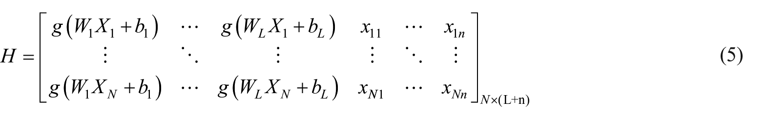
Equation (3) can be expressed as a matrix as follows:

H β = Y

(4)

where $β$ and $Y$ represent the output weight and expected output, respectively. Additionally, H, $β$ and Y can be expressed as follows:

H = {[\begin{matrix} g (W_{1} X_{1} + b_{1}) & \dots & g (W_{L} X_{1} + b_{L}) & x_{11} & \dots & x_{1 n} \\ ⋮ & ⋱ & ⋮ & ⋮ & ⋱ & ⋮ \\ g (W_{1} X_{N} + b_{1}) & \dots & g (W_{L} X_{N} + b_{L}) & x_{N 1} & \dots & x_{N n} \end{matrix}]}_{N \times (L + n)}

(5)

β = {[\begin{matrix} β_{1}^{T} \\ ⋮ \\ β_{L}^{T} \\ β_{L + 1}^{T} \\ ⋮ \\ β_{L + n}^{T} \end{matrix}]}_{(L + n) \times m}

(6)

Y = {[\begin{matrix} y_{1}^{T} \\ ⋮ \\ y_{N}^{T} \end{matrix}]}_{N \times m}

(7)

Furthermore, $\hat{β}$ = H^†Y can be applied to obtain the output weight, where H^† represents the inverse of matrix H.

GWO algorithm

The GWO algorithm¹⁵ uses mathematical modelling of the hierarchy among wolves, as well as their encircling, tracking and attacking behaviour towards other animals, to mathematically express the lives of grey wolves and their methods of capturing prey. Grey wolves usually encircle their prey, and this behaviour can be expressed in the following mathematical form:

\vec{D} = | \vec{C} \cdot \vec{X_{p}} (t) - \vec{X_{(t)}} |

(8)

\vec{X} (t + 1) = \vec{X_{p}} (t) - \vec{A} \cdot \vec{D},

(9)

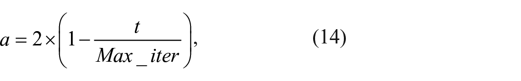
where t is the current iteration, $\vec{A}$ and $\vec{C}$ are coefficient vectors, $\vec{X_{p}}$ is the position vector of the prey and $\vec{X}$ is the position vector of the grey wolf.

Grey wolves find a specific prey and surround it. The commander of the hunting operation is usually known as an alpha wolf, whereas beta and delta wolves may participate in these hunting operations as well, and allow search agents to improve their positions with respect to their initial positions. The position of the search agent is updated as follows:

\vec{D_{α}} = | \vec{C_{1}} \cdot \vec{X_{α}} - \vec{X} |

(10)

When the prey stops moving, the grey wolf attacks it to complete the hunt. To model the approaching prey, $\vec{a}$ must be continuously reduced; the fluctuation range of $\vec{A}$ must also be decreased.

HGS algorithm

The HGS algorithm²¹ can be used for global search and optimisation to avoid arriving at the local optimal solution. The activities and behaviours of a hungry animal can be represented by the following mathematical model:

X (t + 1) = {\begin{matrix} X (t) \cdot (1 + r a n d n (1)), r_{1} < l \\ W_{1} \cdot X_{b} + R \cdot W_{2} \cdot | X_{b} - X (t) |, r_{1} > l, r_{2} > E, \\ W_{1} \cdot X_{b} - R \cdot W_{2} \cdot | X_{b} - X (t) |, r_{1} > l, r_{2} < E \end{matrix}

(11)

where R is a random number located between [−a, a], $r_{1}$ and $r_{2}$ are stochastic numbers between [0,1], t is the current iteration, $W_{2}$ and $W_{1}$ are the current starvation weights, $X_{b}$ represents the global optimal position, $X_{(t)}$ represents the current individual position and $l$ is a set constant. Additionally, E can be calculated as follows:

E = \sec h (| F (i) - B F |), i \in 1, 2, 3, \dots, N

(12)

where $F (i)$ is the fitness of the $i$ th individual and BF is the current best fitness. Additionally, sech() is a hyperbolic function. Furthermore, R can be calculated as follows:

R = 2 \times a \times r a n d - a

(13)

a = 2 \times (1 - \frac{t}{M a x_i t e r}),

(14)

where $r a n d$ is a random number between [0,1] and $M a x_i t e r$ is the number of loops for core optimisation.

To mathematically model hunger in an individual, $W_{1}$ is calculated as follows:

W_{1}^{i} = {\begin{cases} 1, r_{3} > l \\ h u n g r y (i) \cdot \frac{N}{S H u n g r y} \times r_{4}, r_{3} < l' \end{cases}

(15)

Additionally, W₂ is calculated as follows:

W_{2}^{i} = (1 - \exp (- | h u n g r y (i) - S H u n g r y |)) \times r_{5} \times 2

(16)

where hungry is the degree of starvation of the ith unit; N is the total number of units; SHungry represents the sum of the degrees of hunger of all the individuals and $r_{3,} r_{4}, and r_{5}$ are random numbers between [0,1]. Additionally, $h u n g r y (i)$ can be represented as follows:

h u n g r y (i) = {\begin{cases} 0, A L L F i t n e s s = = B F \\ h u n g r y (i) + H, A L L F i t n e s s (i) \neq B F \end{cases},

(17)

where $A L L F i t n e s s (i)$ represents the fitness of the ith individual. Finally, H is calculated as follows:

T H = \frac{F (i) - B F}{W F - B F} \times r_{6} \times 2 \times (U B - L B),

(18)

H = {\begin{cases} L H \times (1 + r), T H < L H \\ T H, T H \geq L H, \end{cases}

(19)

where $r_{6}$ is a random number between [0,1], $F (i)$ represents the fitness of the individual, $W F$ is the present worst fitness value, $U B$ and $L B$ represent the upper and lower bounds of the search space, respectively and $L H$ represents the better bound of H.

Proposed model for classifying the colour differences in dyed fabrics

HGS algorithm improved using GWO

The HGS algorithm possesses excellent features. More specifically, the classification accuracy after convergence, as well as the convergence speed, of the HGS optimisation algorithm is high, and the algorithm can locate the optimal solution globally. The mathematical model of the approaching prey reveals that the random numbers and constants influence whether an animal will approach the prey, as well as the speed of this approach. Therefore, the HGS algorithm continues to arrive at the local optimal solution when seeking the best solution. Additionally, the process of seeking the optimal solution is slow. In contrast, the GWO algorithm retains the current optimal solution, as well as the second and third alternate solutions, owing to the strict hierarchical system of the algorithm. This enhances the ability of the algorithm to search for the optimal solution globally if the current optimal solution falls within the local area. The local optimal solution, as well as the second and third alternative solutions, can be used to search for the global optimal solution, which should rank among the top three solutions. Therefore, GWO is first applied to optimise the HGS algorithm and provide a suitable initial position for this algorithm. The location of the population search agent in the GWO algorithm after optimisation is ranked among the top three. Subsequently, all the population search agents are transferred to the HGS algorithm to initialise its population. At this point, the position of the search agent that has been determined is close to the optimal solution. This effectively prevents the solution from falling within the local area.

Optimised RVFL model for classifying colour differences

Hidden layer offset and input weight are decisive factors that affect the classification performance and stability of RVFL. Therefore, the randomness of the hidden layer offset and input weight will affect the classification accuracy of RVFL when classifying the colour differences of dyed fabrics. To reduce this effect, the HGS algorithm improved using GWO can be applied to optimise the aforementioned parameters and use them to initialise each individual in the population of RVFL. After the cycle, the position that allows the best classification is located and the hidden layer offset and input weight are assigned accordingly in an attempt to improve the stability and classification accuracy of RVFL. The classification error rate of RVFL on the test set is considered to be the fitness function of the optimisation algorithm as follows:

f = \frac{\sum_{i = 1}^{M} T_{i}}{N} 100 %,

(20)

where F and N are the classification error rate and number of samples in the test sets, respectively, $T_{i}$ is classification error in each category and M is the total number of categories.

The proposed model for classifying colour differences using GWO-HGS-RVFL for dyed fabrics is shown in Figure 1. The initial population directly influenced the astringent rate of HGS and ability of the algorithm to avoid arriving at the local optimal solution. The steps following steps are employed by GWO-HGS-RVFL to classify the colour differences in dyed fabrics:

Use high-precision industrial cameras to obtain the images required for the experiment and change the image format.

Calculate the colour differences within the images of the dyed fabrics, and classify the dyed fabrics according to the colour differences. Additionally, combine the features to generate the dataset required for the experiment.

Set the population size N of the GWO, and calculate the dimension of each individual in the population according to: $\dim = (n + 1) \times L$ , where L and n are the numbers of hidden layer and input layer nodes, respectively. Next, set the maximum number of iterations as $T$ .

Update the rank of the wolf pack in GWO and rearrange the position of each search agent to form a matrix. Subsequently, pass the matrix to the hidden layer offset and input weight of RVFL. Use the test set to obtain each search agent in RVFL. Arrange the population positions according to the fitness level, and the alpha wolf is ranked first.

When the positions of all the individuals in the population have been saved and arranged according to the fitness level, the GWO algorithm can be terminated. Use the population positions to initialise the population of the HGS algorithm.

Initialise the other parameters and run the HGS algorithm. Subsequently, calculate the fitness level of the individuals within the population based on the classification accuracy of RVFL.

Update the parameters in the algorithm to calculate the values of hungry, W₁ and W₂, and subsequently calculate the parameters for every individual.

Update the position of every individual.

When the algorithm reaches the maximum number of iterations, save the position of the individual with the best fitness and pass the position as a parameter to RVFL.

Use the test sample to evaluate the classification model based on RVFL to classify the colour differences in dyed fabrics.

Figure 1.

Model classifying the chromatic aberration of dyes using GWO-HGS-RVFL.

Experimental results and analysis

Six other algorithms are compared with the proposed GWO-HGS-RVFL algorithm. These include improved RVFL algorithms based on GWO (GWO-RVFL), HHO (HHO-RVFL), SCA (SCA-RVFL), WOA (WOA-RVFL) and (HGS-RVFL). The operating system used in this experiment is Windows 10, and MATLAB 2021b is used for programming.

Experimental setup

The data set is acquired using the device displayed in Figure 2, and a high-precision colour industrial camera is used to capture the images of the fabrics using standard light sources. The choice of the light source is crucial for classifying the colour differences of dyed fabrics because an inappropriate light source can cause colour distortion. Since this study classifies the colour differences of dyed cotton and polyester fabrics, D65, D50 and A light sources were chosen, which are the three most common light sources in the textile industry.

Figure 2.

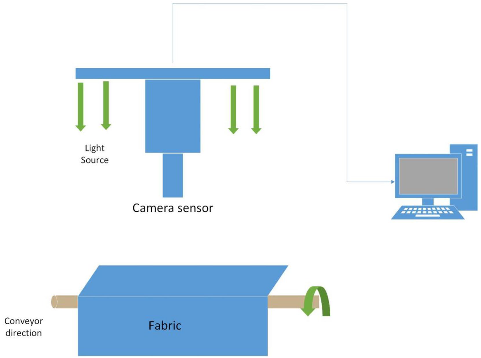
Diagram of the experimental setup.

The obtained images are transferred to a computer for processing to obtain the relevant dataset. The colour difference is calculated as follows:

\begin{matrix} Δ E = [{(\frac{Δ L}{K_{L} \cdot S_{L}})}^{2} + {(\frac{Δ C}{K_{C} \cdot S_{C}})}^{2} + {(\frac{Δ H}{K_{H} \cdot S_{H}})}^{2} + \\ r o t (\frac{Δ C}{K_{C} \cdot S_{C}}) (\frac{Δ H}{K_{H} \cdot S_{H}})]^{\frac{1}{2}} \end{matrix}

(21)

The diagram of the device used in this experiment is shown in Figure 2, and the classification of the colour differences is shown in Table 1.

Table 1.

Intervals used for classifying colour differences.

$E$ (NBS)	Visual intensity	Level
0–0.5	Very weak	1
0.5–1.5	Small	2
1.5–3.0	Evident	3
3.0–6.0	Very evident	4
>6.0	Intense	5

The acquisition process of the dataset is described as follows:

Perform Gaussian denoising on the images captured by the camera, convert the image format, convert the RGB image to an HSV image, and calculate ∆H, ∆S, ∆V. Next, convert the image to the CLELAB colour space and calculate the values of ∆L, ∆a, ∆b.

Calculate the colour difference of each image and classify all the images according to the level assigned to the colour difference.

Combine the features and levels of each image to constitute a dataset. In this experiment, 1400 datasets are constructed. Each dataset has six features and a level category consisting of a total of seven dimensions.

Arithmetic parameter selection

Selecting the activation function

The choice of the activation function of the RVFL neural network affects the accuracy of RVFL. To maximise the accuracy of the experimental results, the number of nodes in the hidden layer of the network is set to 50, and the RVFL neural network applies five-fold cross-validation when using different activation functions. The results obtained are averaged for verification, and the algorithm is executed 10 times. The outcomes of these 10 executions are recorded, and the average value and standard deviation of these outcomes are calculated. As shown in Table 2, when using ‘sig’ as the activation function of RVFL, the classification accuracy of the neural network is only 0.002 smaller than the highest classification accuracy obtained from the ‘sin’ activation function. Additionally, the standard deviation of the classification accuracy obtained using ‘sig’ is the smallest among those obtained using the other activation functions. Based on the classification accuracy, applied ‘sig’ is applied as the activation function of the neural network in the next experiment.

Table 2.

Experimental results of the effect of the activation function of RVFL.

Times	Sig	Sin	Hardlim	Tribas	Radbas	Sign
1	0.982051	0.987179	0.847436	0.950641	0.985256	0.803205
2	0.983974	0.985897	0.845513	0.961538	0.986538	0.853205
3	0.980128	0.984615	0.821795	0.965385	0.982051	0.860897
4	0.983974	0.976923	0.819231	0.967308	0.971795	0.840385
5	0.982051	0.979487	0.836538	0.968590	0.982051	0.848077
6	0.982692	0.988462	0.807692	0.969872	0.977564	0.896795
7	0.981410	0.985256	0.775641	0.772829	0.973077	0.837197
8	0.983333	0.982051	0.805769	0.971795	0.977564	0.833974
9	0.978205	0.984615	0.858974	0.969872	0.978205	0.781410
10	0.980769	0.981410	0.848077	0.965385	0.975641	0.866667
Average	0.981859	0.983590	0.826667	0.966218	0.978974	0.842179
Std	0.001721	0.003394	0.024219	0.006014	0.004665	0.033654

Effect of the number of nodes in the hidden layer of RVFL on the classification accuracy

In RVFL, the number of nodes is a key factor affecting classification accuracy. When the number of nodes is too low, RVFL cannot be fitted, thereby resulting in low classification accuracy. In contrast, when the number of nodes is too high, RVFL will be over-fitted, thereby making the neural network ineffective in classifying data other than training samples. This experiment tests the classification accuracies of the various algorithms according to the number of nodes in the hidden layer. The number of nodes in the hidden layer is increased from 5 to 100, and five-fold cross-validation is performed. Subsequently, the algorithm was executed 10 times and the average value was considered to be the final result. Table 3 and Figure 3 show the classification accuracies of the various algorithms for different numbers of nodes in the hidden layer.

Table 3.

Classification accuracies of various algorithms based on the number of nodes in the hidden layer.

Number of enhancement nodes	GWO-HGS-RVFL	GWO-RVFL	HGS-RVFL	HHO-RVFL	SCA-RVFL	WOA-RVFL
5	0.9703	0.9693	0.9770	0.9577	0.9587	0.9566
10	0.9781	0.9803	0.9866	0.9733	0.9709	0.9754
15	0.9812	0.9808	0.9885	0.9821	0.9784	0.9860
20	0.9836	0.9831	0.9904	0.9862	0.9831	0.9903
25	0.9837	0.9838	0.9908	0.9895	0.9860	0.9904
30	0.9869	0.9871	0.9931	0.9924	0.9871	0.9932
35	0.9874	0.9882	0.9932	0.9945	0.9894	0.9949
40	0.9892	0.9899	0.9946	0.9947	0.9920	0.9951
45	0.9900	0.9902	0.9947	0.9951	0.9936	0.9953
50	0.9903	0.9908	0.9945	0.9951	0.9921	0.9939
60	0.9927	0.9931	0.9950	0.9951	0.9926	0.9943
70	0.9926	0.9931	0.9949	0.9950	0.9937	0.9957
80	0.9912	0.9922	0.9933	0.9951	0.9935	0.9951
90	0.9937	0.9928	0.9944	0.9951	0.9904	0.9944
100	0.9936	0.9913	0.9959	0.9932	0.9957	0.9942

Figure 3.

Effect of the number of nodes on the classification accuracies of various algorithms.

Figure 3 reveals that if the number of nodes in the hidden layer is set between [5,50], the classification accuracy of a neural network increases with the increase in the number of nodes. However, when the number of nodes is set between [50,100], the classification accuracy increases relatively slowly and subsequently stabilises. After comprehensively analysing the images and tables we conclude that when the number of nodes reaches 80, the classification accuracy becomes relatively stable; therefore, the number of nodes in the hidden layer of the model was set to 80 in this experiment. In addition, we can conclude that the classification accuracies of HGS-RVFL and GWO-HGS-RVFL are better than those of the other algorithms when the number of nodes in the hidden layer is small.

Parameters of the improved HGS algorithm using GWO

Population size and the number of iterations play an important role in an optimisation algorithm and setting these parameters improperly consumes unnecessary resources. If these parameters are too large, the algorithm will execute for an extended duration and increase the time cost. However, if these parameters are too small, the algorithm will produce poor results, thereby resulting in low classification accuracy. In this experiment, different values are set for the two parameters, and different classification accuracies are obtained. These classification accuracies are then compared to obtain the best combination of the number of iterations and population size. The population size can assume five possible values, that is, 10, 20, 30, 40 or 50, and the number of iterations can assume six possible values, that is, 5, 10, 15, 20, 25 or 30. Additionally, 30 combinations of these two parameters are possible. We applied each combination to GWO-HGS-RVFL, averaged the results using five-fold cross-validation, and the final result obtained is the average of 10 executions of the algorithm.

Figure 4 displays the influence of different combinations of the two parameters on the classification accuracy of the algorithm, which is represented by the bubbles in the image. When the population number or number of iterations increases, the area of the bubble increases. For fixed population size, with the increase in the number of iterations, the classification accuracy of the algorithm gradually improves. Additionally, for a fixed number of iterations, with the increase in the population size, the classification accuracy of the algorithm improves gradually. However, when the population size is set to 40 or 50, the classification accuracy of the algorithm does not change substantially; therefore, we set the population size to 40. Because the convergence speeds of different algorithms are different, the number of iterations is set to 60 in this experiment.

Figure 4.

Classification accuracy of the algorithm according to the population size and number of iterations.

Parameter settings for the various algorithms

To ensure the credibility of the results, the parameter settings are consistent with those of GWO-HGS-RVFL. The activation function of RVFL is set to ‘sig’, number of nodes in the hidden layer is set to 80, population size in the optimisation algorithm is set to 40, and number of iterations is set to 60.

Discussion of the results obtained from the algorithms

This experiment uses five-fold cross-validation for the algorithms, and the obtained results are averaged. The algorithms are executed 10 times to reduce the randomness of the results and improve their credibility. Table 4 displays the minimum value (Min), maximum value (Max), standard deviation (Stdv) and average value (Avg) obtained by executing various algorithms 10 times.

Table 4.

Comparison of the experimental results obtained from various algorithms (the optimal values are displayed in bold).

Measure	GWO-HGS-RVFL	GWO-RVFL	HGS-RVFL	HHO-RVFL	SCA-RVFL	WOA-RVFL
Max	0.9955	0.9936	0.9948	0.9955	0.9937	0.9954
Min	0.9937	0.9915	0.9935	0.9922	0.9905	0.9922
Avg	0.9945	0.9925	0.9940	0.9937	0.9921	0.9945
Stdv	0.0006	0.0007	0.0004	0.0009	0.0009	0.0009

Convergence, significance and stability analyses of the algorithms

Stability analysis

Figure 5 shows a box diagram of the classification error rate of the algorithms used in this experiment. The algorithm uses five-fold cross-validation results to average the error rate of each algorithm, and the algorithm was executed 10 times. The classification error rate obtained is saved in the box and displayed in the form of a pattern diagram. The upper and lower horizontal lines of each box represent the maximum and minimum error rates obtained from the 10 executions of the algorithms. The open circles are abnormal points, and the lower and upper borders of each box represent the one-quarter and three-quarter digits of the error rates, respectively. The green horizontal lines inside the boxes represent the medians of the error rates. From the lengths of the boxes in Figure 5, the stability of GWO-HGS-RVFL can be observed to be substantially better than those of GWO-RVFL and WOA-RVFL, slightly better than that of HHO-RVFL, and similar to those of SCA-RVFL and HGS-RVFL. Additionally, Table 3 and Figure 5 reveal that the proposed GWO-HGS-RVFL algorithm in this study possesses a small error and good stability.

Figure 5.

Classification error rate box plot of the various algorithm.

Algorithm convergence analysis

In Figure 6, the convergence speed of GWO-HGS-RVFL is compared with those of the other algorithms, in which the classification error rate is used to express the fitness. From the figure, we can clearly observe that the astringent speed of GWO-HGS-RVFL is much higher than those of the neural networks optimised using other algorithms. Additionally, when the number of iterations increases gradually, the fitness of GWO-HGS-RVFL is very low. The performance of this algorithm is excellent and obtained fitness is nearly the same as the final fitness of HGS-RVFL. GWO-HGS-RVFL reaches the smallest degree of fitness in the smallest number of iterations. The comprehensive analysis confirmed the superiority of GWO-HGS-RVFL.

Figure 6.

Convergence analysis results of the various algorithms.

The no lunch theory²⁴ indicates that an optimisation algorithm cannot perform well when all its parameters are optimised. Therefore, we initialised the population of the HGS algorithm using GWO to improve the convergence speed of HGS and avoid the local optimal solution, thereby improving the classification accuracy of RVFL.

Difference between algorithms

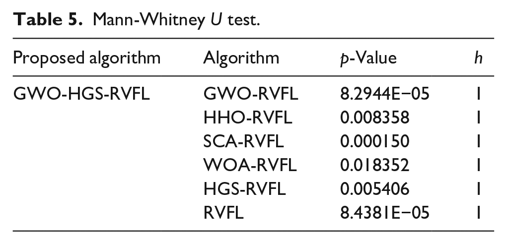
To determine the difference between GWO-HGS-RVFL and other algorithms, Mann-Whitney U test is used to analyse the experimental results. Similar to previous experiments, to increase the reliability of the results, we use five-fold cross-validation, each algorithm is executed 10 times, and the results of the 10 executions are averaged.

Table 5 reveals that the p-value of GWO-HGS-RVFL and the other algorithms is less than 0.05 and h is equal to one for all the algorithms; therefore, considerable differences exist between GWO-HGS-RVFL and the other algorithms. The experimental results prove that GWO optimises HGS and subsequently optimises RVFL, which results in obvious advantages over using HGS alone.

Table 5.

Mann-Whitney U test.

Proposed algorithm	Algorithm	p-Value	h
GWO-HGS-RVFL	GWO-RVFL	8.2944E−05	1
	HHO-RVFL	0.008358	1
	SCA-RVFL	0.000150	1
	WOA-RVFL	0.018352	1
	HGS-RVFL	0.005406	1
	RVFL	8.4381E−05	1

Conclusion

This study proposed an algorithm for the classification of dyes based on an improved HGS optimisation of the RVFL neural network. From the experimental results, we can draw the following conclusions:

The convergence analysis and corresponding graphs reveal that the HGS algorithm improved using GWO has a better convergence speed and higher accuracy than those of the other algorithms.

The stability analysis and box diagram reveal that the HGS algorithm improved using GWO has better stability than those of other algorithms.

GWO can be used to initialise the population of HGS. such that the probability of HGS arriving at the local optimal solution is greatly reduced.

Additionally, obvious differences exist between GWO-HGS-RVFL and other algorithms, and GWO-HGS-RVFL is superior to the other algorithms.

In the future, further research will be conducted on the application of the proposed algorithm in enterprises. Additionally, we will attempt to solve the real-time problems associated with online production at enterprises and process large amounts of data required for detecting and classifying colour differences.

Footnotes

Declaration of conflicting interests

The author(s) declared no potential conflicts of interest with respect to the research, authorship, and/or publication of this article.

Funding

The author(s) disclosed receipt of the following financial support for the research, authorship, and/or publication of this article: This work is supported by Zhejiang Provincial Department Education (No. FG2020056) and Zhejiang Provincial Key Research and Development Programme (No. 2021C03013).

ORCID iD

Zhiyu Zhou

References

Shanbeh

Khalili

Hajrasouliha

, et al. Evaluation of color difference, whiteness, and luster of multifilament polyester woven fabrics. J Eng Fibers Fabr 2014; 9(3): 168–175.

Cui

Xue

Liu

, et al. Intelligent manufacturing of color blended yarn: color matching algorithm and manufacturing process through computer numerically controlled ring spinning system. J Eng Fibers Fabr. Epub ahead of print 1 January 2021. DOI: 10.1177/15589250211006539.

Wang

Jiang

, et al. Establishment of a color tolerance for yarn-dyed fabrics from different color-depth yarns. Color Res Appl 2022; 47(1): 225–235.

Xin

Zhang

, et al. Color texture classification of yarn-dyed woven fabric based on dual-side scanning and co-occurrence matrix. Text Res J 2017; 87(15): 1883–1895.

Wang

Jing

JF.

Application of improved back propagation algorithm in color difference detection of fabric. Color Res Appl 2015; 40(3): 311–317.

Zhang

Yang

Evaluation model of color difference for dyed fabrics based on the support vector machine. Text Res J 2014; 84: 2184–2197.

Wang

Zhang

Wang

, et al. A computer vision-based system for automatic detection of misarranged color warp yarns in yarn-dyed fabric. Part III: yarn layout proofing. J Text Inst 2020; 111: 1614–1622.

Xie

, et al. An algorithm for online detection of colour differences in warp knitted fabrics. J Text Inst 2022; 113: 159–165.

Barua

Patil

Desai

P D

, et al. Deep learning-based smart colored fabric defect detection system. Adv Intell Syst Comput 2020; 1155: 212–219.

10.

Zhang

Dong

Wang

, et al. Advances in multimodal data fusion in neuroimaging: overview, challenges, and novel orientation. Inf Fusion 2020; 64: 149–187.

11.

Zhang

Satapathy

Guttery

, et al. Improved breast cancer classification through combining graph convolutional network and convolutional neural network. Inf Process Manag 2021; 58: 102439.

12.

Wang

Govindaraj

Górriz

, et al. Covid-19 classification by FGCNet with deep feature fusion from graph convolutional network and convolutional neural network. Inf Fusion 2021; 67: 208–229.

13.

Zhou

Liu

Zhang

, et al. Colour difference classification for dyed fabrics based on differential evolution with dynamic parameter selection to optimise the output regularisation extreme learning machine. Fibres Text East Eur 2021; 29(3(147)): 97–102.

14.

Shi

Yang

Color difference classification of dyed fabrics via a kernel extreme learning machine based on an improved grasshopper optimization algorithm. Color Res Appl 2021; 46(2): 388–401.

15.

Mirjalili

Lewis

Grey wolf optimizer. Adv Eng Softw 2014; 69(3): 46–61.

16.

Zhou

Zhang

, et al. Fabric wrinkle level classification via online sequential extreme learning machine based on improved sine cosine algorithm. Text Res J 2020; 90(17–18): 2007–2021.

17.

Mirjalili

Lewis

The whale optimization algorithm. Adv Eng Softw 2016; 95: 51–67.

18.

Liu

Yang

Color constancy computation for dyed fabrics via improved marine predators algorithm optimized random vector functional-link network. Color Res Appl 2021; 46(5): 1066–1078.

19.

Heidari

Mirjalili

Faris

, et al. Harris hawks optimization: algorithm and applications. Future Gener Comput Syst 2019; 97: 849–872.

20.

Shi

Yang

Fabric wrinkle evaluation model with regularized extreme learning machine based on improved Harris hawks optimization. J Text Inst 2022; 113(2): 199–211.

21.

Yang

Chen

Heidari

, et al. Hunger games search: visions, conception, implementation, deep analysis, perspectives, and towards performance shifts. Expert Syst Appl 2021; 177: 114864.

22.

Shi

Yang

Clothing image classification with a dragonfly algorithm optimised online sequential extreme learning machine. Fibres Text East Eur 2021; 29(3(147)): 91–96.

23.

Pao

Park

Sobajic

DJ.

Learning and generalization characteristics of the random vector functional-link net. Neurocomputing 1994; 6(2): 163–180.

24.

Wolpert

Macready

WG.

No free lunch theorems for optimization. IEEE Trans Evol Comput 1997; 1: 67–82.

Classifying colour differences in dyed fabrics using an improved hunger games search optimised random vector functional link

Abstract

Keywords

Introduction

Preliminaries

RVFL network

GWO algorithm

HGS algorithm

Proposed model for classifying the colour differences in dyed fabrics

HGS algorithm improved using GWO

Optimised RVFL model for classifying colour differences

Experimental results and analysis

Experimental setup

Arithmetic parameter selection

Selecting the activation function

Effect of the number of nodes in the hidden layer of RVFL on the classification accuracy

Parameters of the improved HGS algorithm using GWO

Parameter settings for the various algorithms

Discussion of the results obtained from the algorithms

Convergence, significance and stability analyses of the algorithms

Stability analysis

Algorithm convergence analysis

Difference between algorithms

Conclusion

Footnotes

Declaration of conflicting interests

Funding

ORCID iD

References