Sage Journals: Discover world-class research

Abstract

Fiber/matrix debonding behavior of steel fiber composites is analyzed using a parametric finite element modeling procedure and compared with conventional composites with carbon and glass fibers. Cohesive surfaces are applied to fiber–matrix interface to simulate the debonding behavior, while the interface strength properties of steel fiber are obtained with and without surface treatment. The effect of various parameters on the debonding behavior is investigated, including stress concentrations, fiber diameter, fiber shape, and fiber volume fraction, using the parametric model. The influence of stress concentrations is determined to be much lower than the debonding strength. Debonding damage is more evident in larger fibers compared to smaller ones. Earlier and sudden interface separation is observed with the polygonal steel fibers compared to the circular ones. Increase in the fiber volume ratio increases the debonding opening distance but does not affect the opening angle significantly. The results can be useful for assessing possibilities to use steel fibers to increase toughness of the composites in comparison with glass and carbon reinforcement.

Keywords

Micro-scale finite element method steel fiber composites stress concentrations fiber/matrix debonding

Introduction

Fiber-reinforced composite materials have been used for many decades in many technical areas such as aviation, automotive, and construction industry due to their tailored properties. Using steel fibers as reinforcement was recently developed as an alternative to carbon and glass fiber. Steel fibers bring a remedy to a well-known lack of ductility in composites while still providing high stiffness to composite structure.^1–3 However, together with a drawback of the extra weight they add to the structure, these composites are prone to high stress concentrations in the fiber–matrix interface due to the high stiffness mismatch between the fiber and the matrix.⁴

Using a different fiber than the conventional glass and carbon requires the damage behavior to be investigated in detail. It is known that while the resistance to damage under loading in fiber direction is quite high in unidirectional composites, this is not the case in transverse loading. The damage evolution generally starts with crack formations or debonding in fiber–matrix interface in micro-scale, and these cracks evolve through the matrix.^5,6 After they coalesce, the cracks may cause the loss of structural integrity or at least the decrease of stiffness in macro-scale, which may, in its turn, cause the other components to carry unexpected high loads. Thus, the investigation of composite failure in micro-scale is quite important as the micro-scale failure is the root cause of such macro-scale failure modes. In the case of steel fibers, as high stress concentrations occur under transverse loading, fiber/matrix debonding is a crucial failure mode that should be considered in design.¹

Fiber/matrix debonding has been observed as a common failure mode in micro-scale as shown in Figure 1. Thus, there have been some studies to model this behavior to predict macro-scale failure. In Maligno et al.,⁷ empirical damage models are applied to determine the fiber/matrix debonding under mechanical and thermal loads. In these models, the matrix and all of the fibers were assumed to be separated, suddenly. However, in reality, fiber/matrix debonding is a stepwise process and it occurs gradually along the surface of the fiber while the stress distribution in the matrix is changing continuously. In order to observe this debonding evolution, numerical methods such as finite element method (FEM) are applied on the micro-scale, using the cohesive zone modeling (CZM) technique. In Ghosh et al.,⁸ Voronoi cell element is used to model the fiber/matrix debonding with cohesive zone technique with the addition of springs in tangential and normal directions at the interface. Canal et al.⁹ used CZM to determine the damage in micro-scale under three-point bending. Garcia et al.¹⁰ included contact and fracture mechanics models in addition to the cohesive zone to investigate the failure under transverse loading. Among more recent studies, Mora et al.¹¹ analyzed 0° and 90° laminae with a representative volume element (RVE). A damage mode is added to the fiber/matrix debonding to simulate the transverse failure mode. Although it was mentioned that the results are similar with the experiments, the matrix model is extremely simplified and needs to be developed. In Naya et al.,¹² a similar study is performed with unidirectionally oriented carbon fiber composites. In addition to transverse tensile loading, compressive and in-plane shear load are applied and the failure under these loading types is investigated.

Figure 1.

Fiber/matrix debonding shown in (a) Wood and Bradley,¹³ (b) Suresh et al.,¹⁴ and (c) Callens et al.¹

As a new type of composite material, the fiber/matrix debonding of steel fiber composites has not been yet studied numerically. Thus, the aim of this study was to investigate this behavior in steel fiber composites in comparison with the conventional carbon/glass fiber ones and to understand the effect of various parameters such as stiffness mismatch, interface strength, and fiber volume fraction on the debonding behavior. Due to their manufacturing process, steel fibers can have a polygonal cross-sectional shape.¹⁵ Thus, the effect of the shape of the fiber is another parameter considered in the study.

In the work by Sabuncuoglu et al.,⁴ the present authors studied the effect of steel fiber parameters on stress concentrations under transverse loading. In the present work, the focus is given to the debonding behavior of steel fibers. Initially, the cohesive zone application methodology is validated via a comparison with a previous study. Then, the debonding of steel fibers, with and without surface treatment, is compared with the conventional glass- and fiber-reinforced composites. The comparison shows the improvement of debonding behavior with the surface treatment but lacks a scientific conclusion as many parameters change simultaneously while comparing different fiber types with each other. Thus, parametric studies are performed to reveal the effects of certain parameters such as stress concentrations (stiffness contrast), fiber size, fiber shape, and fiber volume fraction on the fiber/matrix debonding mode and the expected failure initiation in the matrix. The model in this study claims simulation of the local debonding process, which is the first step in the succession of the damage development leading to failure. The later stages such as crack formation and crack growth inside the matrix are not considered here and left for a future study. The entire study is performed using commercially available ABAQUS® finite element software and by scripting in Python® programming language for parametric modeling.

The article starts with the explanation of the models (section “Micromechanical model”). In section “Modeling of damage behavior and the determination of damage parameters,” the application of damage behavior is presented. In section “Verification of the numerical model,” the validation of the developed model is presented with the verification of some material parameters used in the study. In section “Results,” the results revealing the effect of various parameters in the design are presented. Finally, in section “Conclusion,” conclusions obtained from the study are discussed.

Micromechanical model

Analysis of fiber/matrix debonding requires a micromechanical model to be generated where fiber and matrix regions are modeled separately. Various distributions of fibers can be investigated at this stage. In a real composite, the fibers are distributed randomly in the matrix, and there are some studies where the debonding is analyzed in this way.^11,12,16 In the present work, regular fiber packing is used, as our focus is on the details of the interface behavior considering the material and interface parameters, rather than on assessing the composite strength and fracture resistance in general. Hexagonal packing of fibers is a widely accepted packing methodology to analyze fiber–matrix interactions^17–19 and is used in this study.

Two values of fiber volume fraction (vf = 0.4 and 0.6) are considered as these are generally the upper and lower limits in composite design. The dimensions of the RVE are defined parametrically, depending on the fiber diameter. In the case of steel fibers, some of the models are generated with hexagonal cross-section to study the effect of cross-sectional shape. The dimensions of hexagonal fibers are adjusted to have the same cross-sectional area as their circular counterparts.

Transverse loading is applied on the right edge of the RVE. Application of transverse strain causes different stresses in the micromechanical model due to the variance in the fiber type and fiber volume fraction. Thus, the results would mislead the designer as more stresses are applied to the stiffer material. For this reason, loading is applied via transverse force on one side of the model. In order to have the same displacement on the right edge of the model, the following procedure is applied. First, a reference point is generated arbitrarily at 1.5 times the width of the model. Then, a point load is applied to this reference point, which is determined to obtain the required average transverse stress. Then, equation constraints are defined for each node on the right edge to have the same displacement in the x-direction with this reference point. A value of 80 MPa was determined to be enough to cover fiber–matrix separation and expected failure in the matrix for all of the composite types considered in this study. Note that a crack in the matrix may occur and evolve much earlier than this value. The time steps for the application of the load are left to the solver as it would be very difficult to predict the best time step for each model type.

Due to the quarter symmetric nature of the model, the left and bottom sides of the RVE are fixed in x- and y-directions, respectively. The top edge of the model should contract with the applied load due to Poisson effect. For this purpose, a similar procedure, performed for the nodes on the right edge, is applied for the nodes at the top edge of the model, following the studies of Maligno et al.⁷ and Sun and Vaidya.²⁰ Another reference point is generated at about 1.5 times the height of the model. Then, equation constraints are defined for each node at the top edge to have the same displacement in the y-direction. However, this time, the reference point is left free without any boundary conditions. This causes the reference point and the connected top-edge nodes to move in the −y-direction together due to the Poisson contraction caused by the transverse load. Examples of models with the mesh structure for circular and hexagonal shape fibers for vf = 0.6 are shown in Figure 2 with the boundary conditions shown in Figure 2(a).

Figure 2.

Models with hexagonal packing of fibers with (a, c) circular and (b, d) hexagonal cross-sections.

Four-noded quadrilateral and three-noded triangular linear generalized plain strain elements with full integration were used in the mesh (CPEG4 and CPEG3, respectively). The mesh-seed, especially at the fiber–matrix interface, was assigned in a way to obtain elements with good aspect ratio. Three-noded triangular elements are present in the mesh, which are known to have low accuracy. However, they exist rarely and away from the interface so that they do not contribute to the results. The mesh properties are provided in Table 1.

Table 1.

Properties of the applied mesh (vf = 0.6).

$v f$	Fiber shape	Total number of elements	Total number of nodes	Approximate dimensions of rectangular interface elements (see Figure 2)
0.6	Circular	6442	6665	0.26 µm × 0.15 µm
0.6	Hexagonal	6080	6318
0.4	Circular	7856	8073
0.4	Hexagonal	7584	7802

The models are generated separately for each fiber type with their individual material properties (Table 2).⁴ Epoxy is used as the matrix material with E = 3 GPa and $υ = 0.4$ . Trial analyses showed that high strain analyses should be performed to cause debonding in micro-scale. Thus, the stress–strain curve of epoxy covering the elasto-plastic material behavior region is implemented on the model in tabular form which was taken from Okabe et al.²¹

Table 2.

Elastic properties of the fibers.

Steel	E-Glass	Carbon (IM-7)
E = 193 GPa $υ = 0.3$ d = 30 µm	E = 72 GPa $υ = 0.25$ d = 10 µm	E_L = 276 GPa E_T = 10.3 GPa G_TT = 3.8 GPa G_LT = 27.9 GPa $υ_{L T} = 0.26$ d = 7 µm

d, diameter; E, Young’s modulus; $υ$ , Poisson’s ratio; $L$ and $T$ , longitudinal and transverse directions, respectively.

Modeling of damage behavior and the determination of damage parameters

Various methodologies are present in the finite element method to represent the damage and fracture aspects in composite materials. Implementation of CZM has been a popular approach which can be implemented directly in commercially available finite element software. In this method, failure of interface bond between two surfaces is characterized by the degradation of interface stiffness when a certain criterion related to displacement or traction is reached. CZM is a convenient method to investigate crack initiation and propagation together, which cannot be achieved with other methods such as J-integral. The difficulties encountered are the proper definition of interface properties. In addition, convergence difficulties are encountered in this type of analysis. Dependence on element size in the finite element model is also a known issue while implementing CZM.²²

In ABAQUS, cohesive zone can be defined either by cohesive elements or by cohesive surfaces. In the former one, special purpose elements are defined in the interface, which are deleted when separation criterion is achieved. In the latter one, contact conditions are defined at the interface and the contact is released according to the damage criteria. Trial analysis showed some convergence difficulties during the element deletion process, so cohesive surface was chosen for the modeling of the interface separation.

In the cohesive zone approach, when a separation force/displacement is applied, the traction first increases until a maximum is reached and then reduces to zero, which results in complete separation (Figure 3(a)). Similar curves should be defined for the separation under shear, and these curves should be combined with a mixed-mode behavior.²³ The area under the curve is called the fracture energy. Sufficient parameters are needed to define these curves. They are presented in Figure 3(b) for normal (red) and shear (blue) directions. The part of the curve before the maximum load is called the damage initiation zone, while the other side is called the damage evolution zone.

Figure 3.

Cohesive zone modeling: (a) typical traction–separation curve and (b) parameters needed to be determined for the analysis.

The combined effect of mixed-mode loading can be defined by various formulations. The quadratic traction criterion was determined to be the most frequently used method for damage initiation criteria in fiber/matrix debonding according to the previous related studies.^11,12,24 In all of them, the shear parameters in Mode II and Mode III are assumed to be equal. The quadratic traction criterion is calculated as in equation (1)

{(\frac{t_{n}}{N_{m a x}})}^{2} + {(\frac{t_{s}}{T_{m a x}})}^{2} + {(\frac{t_{t}}{T_{m a x}})}^{2} = 1

(1)

where $t_{n}$ is the traction along the normal direction; and $t_{s}$ and $t_{t}$ are the tractions along the two shear directions. $N_{m a x}$ and $T_{m a x}$ are the normal and shear strengths of the interface, respectively, which should be given as input.

For steel fibers, $N_{m a x}$ is taken from dolly tests performed for steel–epoxy adhesion.²⁵ Tests were performed with two configurations. In the first one, epoxy is cured directly on the steel plate, whereas in the second one, APS ((3-aminopropyl)triethoxysilane) surface treatment is applied to the surface of fibers. The maximum stresses obtained by these tests are 30 and 63 MPa, respectively. Both of these conditions are considered for analysis in order to observe the difference between these high and low interface strength cases.

Evolution of damage is described as linear softening (see Figure 3(b)), similarly as in previous works^16,26,27 for other types of fibers. No data were found for interfacial fracture toughness between steel fibers and epoxy. In Mora et al.,¹¹ the fracture energy of epoxy (100 J/m²) is used for epoxy–glass interface for all three directions. In Naya et al.,¹² different values of fracture energy are used for carbon–epoxy interface (280, 790, 790 J/m² for $G_{I C}$ , $G_{I I C}$ , and $G_{I I C}$ , respectively). Trial analyses revealed that the fracture energy values around this scale did not affect the results significantly (see section “Analysis of Fracture Energy Difference”). Thus, the same value is used for the other fiber types in order to be able to compare the results more accurately. The mode 3 fracture energy $(G_{I I C})$ does not have any interaction with the results as generalized plane strain elements are used. Nevertheless, it is implemented as the software requires this input and to be a reference for possible future study with three-dimensional (3D) elements and mode 3 loading.

Measurement of the interfacial shear strength presents serious difficulties. In order to determine the shear strength $(T_{m a x})$ , initially, previously performed micro-droplet test results were considered.²⁸ It was observed that relatively low strength values are obtained from these tests compared to the ones obtained with other test types such as fiber push-out tests. This was also the case when micro-droplet test was applied to carbon–epoxy interface.^29,30 The reason is associated with the curing of small amount of resin and the dependence on the droplet shape. Due to this reason, the micro-droplet results were considered unreliable and not used in the present work. The value of the shear strength is suggested to be 1.5 times the normal strength observed in Ogihara and Koyanagi.³¹ This ratio was observed for both the carbon and glass fibers in the literature.^11,12 Therefore, $N_{m a x}$ values for steel fibers are multiplied by 1.5 and used as $T_{m a x}$ in this study.

The penalty stiffness in the cohesive zone traction-separation law is not a physical parameter and controls the calculation convergence. The value used in Mora et al.¹¹ (5 × 10⁷ MPa/µm) was used in this study. Another such parameter is the viscous coefficient. A value of µ = 1 × 10⁻⁵ is used for this coefficient after trial analysis (see the verification in section “Verification of the numerical model”).

As mentioned, the debonding behavior of steel fibers is compared with the conventional glass and carbon fiber, the interface properties of which are taken from Mora et al.¹¹ and Naya et al.,¹² respectively. All the interface properties are summarized in Table 3 showing each model with the model code used in the further sections of the article. As an example, a code S-t-h-0.6 means a model with hexagonally shaped (h) steel fibers (S) with APS surface treatment (t) and the composite fiber volume ratio of 0.6.

Table 3.

Material codes for various types of models.

Material code	Surface code	Fiber Material	$N_{\max}$ (MPa)	$T_{\max}$ (MPa)	$G_{IC}$ (J/m²)	$G_{IIC}$ (J/m²)	$G_{IIIC}$ (J/m²)
S	b	Steel (without treatment)	30	45	100	100	100
S	t	Steel (APS treatment)	63	95	100	100	100
G		Glass	50	75	100	100	100
C		Carbon	42	63	100	100	100
Material code		Explanation
c/h		Circular/hexagonal cross-section (fibers)
0.4/0.6		Fiber volume ratio

APS: 3-aminopropyl)triethoxysilane.

Verification of the numerical model

Determination of the viscous regularization coefficient

One of the parameters that is very difficult to determine is the viscous regularization coefficient which is implemented on the model to prevent unstable crack growth due to softening. If this coefficient is too high, it may produce non-physical results. Low values can prevent the analysis to converge.

Analyses are performed with various viscous coefficient values to observe the difference. The model S-b-c-0.6 is used as a benchmark in the analyses. The values lower than µ = 1 × 10⁻⁵ caused numerical non-convergence. The results with three viscous coefficient values larger than this value are presented in Figure 4. According to the results, the viscous coefficient of 1 × 10⁻³ seems to be too high, causing a stress distribution too different from the results with the lower µ values. Thus, the default value 1 × 10⁻⁵ is decided to be used in the subsequent analysis.

Figure 4.

Distribution of maximum principal stresses (MPa) at applied $σ_{x} = 43 M P a$ with viscous coefficient µ: (a) 1 × 10⁻³, (b) 1 × 10⁻⁴, and (c) 1 × 10⁻⁵.

Verification of the mesh structure

It is known that the cohesive zone behavior can be strongly influenced by the mesh structure.²² Thus, various analyses were performed with different mesh densities to analyze the difference. Again, the model S-b-c-0.6 is used as a benchmark. The analyses were initially performed with the mesh structure given in Figure 5(a). Then the mesh density is increased. As no significant change in the stress field is observed (Figure 5), the mesh shown in Figure 5(a) was used for the subsequent analysis.

Figure 5.

Distribution of maximum principal stresses (MPa) at applied $σ_{x} = 43 M P a$ with (a) coarse, (b) normal, and (c) fine mesh.

Verification of the cohesive zone application

In order to confirm that the application methodology is correct, it was decided to replicate a similar model from the literature where fiber–matrix interface bonding is analyzed with cohesive zone. Nearly in each of the studies in the literature related to cohesive zone, there exists some missing information about the parameters used for CZM and preventing replication of the model. The model with the least missing information and closest to the present study is found in the work performed by Kushch et al.,¹⁶ which was used as the benchmarking case.

In section 4.2 of that paper, a single-fiber model is constructed with cohesive zone defined around the fiber. The model parameters are similar to the parameters described in sections “Micromechanical model” and “Modeling of damage behavior and the determination of damage parameters,” with the exception that the evolution of damage is defined using linear form instead of quadratic. The study also had some missing information such as viscous regularization coefficient (µ) and initial contact stiffness ( $K$ ), so these were assumed by some trial analyses considering the convergence requirements. In contrast to our present study, where transverse load is applied as a point load in the x-direction (see Figure 2), the load is applied as negative pressure in the y-direction with an unknown step size in that paper. Quarter symmetry geometry is used in the present validation model, which is equivalent to the full fiber geometry in Kushch et al.¹⁶

The distribution of the stresses obtained in Kushch et al.¹⁶ and the present validation model is shown in Figure 6 for two dimensionless pressure values. Due to using different software in the analyses, the color spectrum is slightly different in Kushch et. al.¹⁶ and the present study. According to Figure 6(a) and (b), where a dimensionless pressure of −0.85 is applied, the damage is about to start and high stresses are observed at a similar singular location around the fiber for both models. The distribution bands follow a very similar trend. Slight difference is observed in the distribution of the stresses near the crack onset location on the fiber side. When the pressure is increased to −1, the distribution of stresses in the vertical axis is not as similar as the condition just before the debonding starts (Figure 6(c) and (d)). However, the major difference is the stress inside the fiber which is not important for the analysis of matrix stresses. The stresses are in similar range, and this much difference is considered acceptable considering the unknown parameters not mentioned in the original study. Nevertheless, fiber/matrix debonding occurs until the same angular location is reached for both models.

Figure 6.

Distribution of stresses in the y-direction in (b, d) the validation model and (a, c) Kushch et al.¹⁶

Results

Comparison of steel fibers with glass and carbon fibers

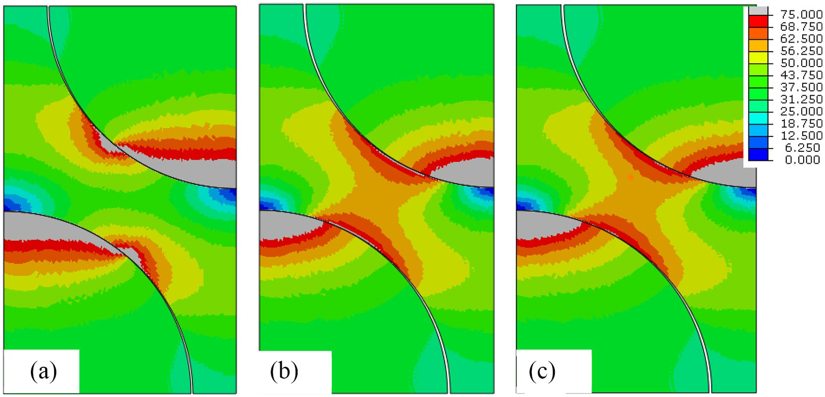
With the applied load of 80 MPa, the analysis results are obtained for all fiber types with automatic time steps. The distribution of the principal stresses for various fiber types is shown in Figure 7 with the applied transverse stress ( $σ_{x}$ ). The distribution of the stresses is provided at the load, corresponding to the appearance of stress of 75 MPa somewhere in the matrix, which is a typical tensile strength ( $S_{u t s}$ ) for epoxy.³² Thus, the applied load was different for each model.

Figure 7.

Distribution of maximum principal stresses for the models when $S_{u t s} = 75 M P a$ is reached in the matrix: (a) S-b-c-0.6, (b) G-c-0.6, (c) C-c-0.6, (d) S-t-c-0.6, and (e) S-b-c-0.6 zoomed to show the amount of debonding. “x” shows the limit of the debonded area.

The results reveal the amount of debonding reached for each fiber type. At the location where debonding on the fiber stops (separation point shown by “x”), there is a stress concentration in the matrix. For all of the models with different fiber types, $S_{u t s} = 75 MPa$ is reached at this separation point, which is also observed in Kushch et al.¹⁶ Thus, after this amount of debonding, it is expected that a crack will be formed and will grow through the inner parts of the matrix.

When the distributions are investigated, we observe that at the load when $S_{u t s}$ for epoxy is reached, the amount of debonding on the fiber–matrix interface is maximum for the steel fiber without plating. When the plating is issued on the fiber, $S_{u t s}$ is reached with a much smaller debonded region due to the strong bonding. Another point to mention is the distribution of stresses in the fiber. We can observe that more stresses are taken by the fiber in the case of treated steel fiber and the stresses are distributed evenly inside the fiber. On the contrary, for blank (untreated) steel, high stresses are observed at a certain small region of the fiber and most of the fiber is not stressed. This is an unwanted situation as the stress is not distributed throughout the fiber. Carbon and glass fiber composites lie between these two extremes. It is important to mention that in these figures, the stresses applied to each composite are different as the distributions are obtained at the instant $S_{u t s}$ is reached in the matrix, which is different for each composite.

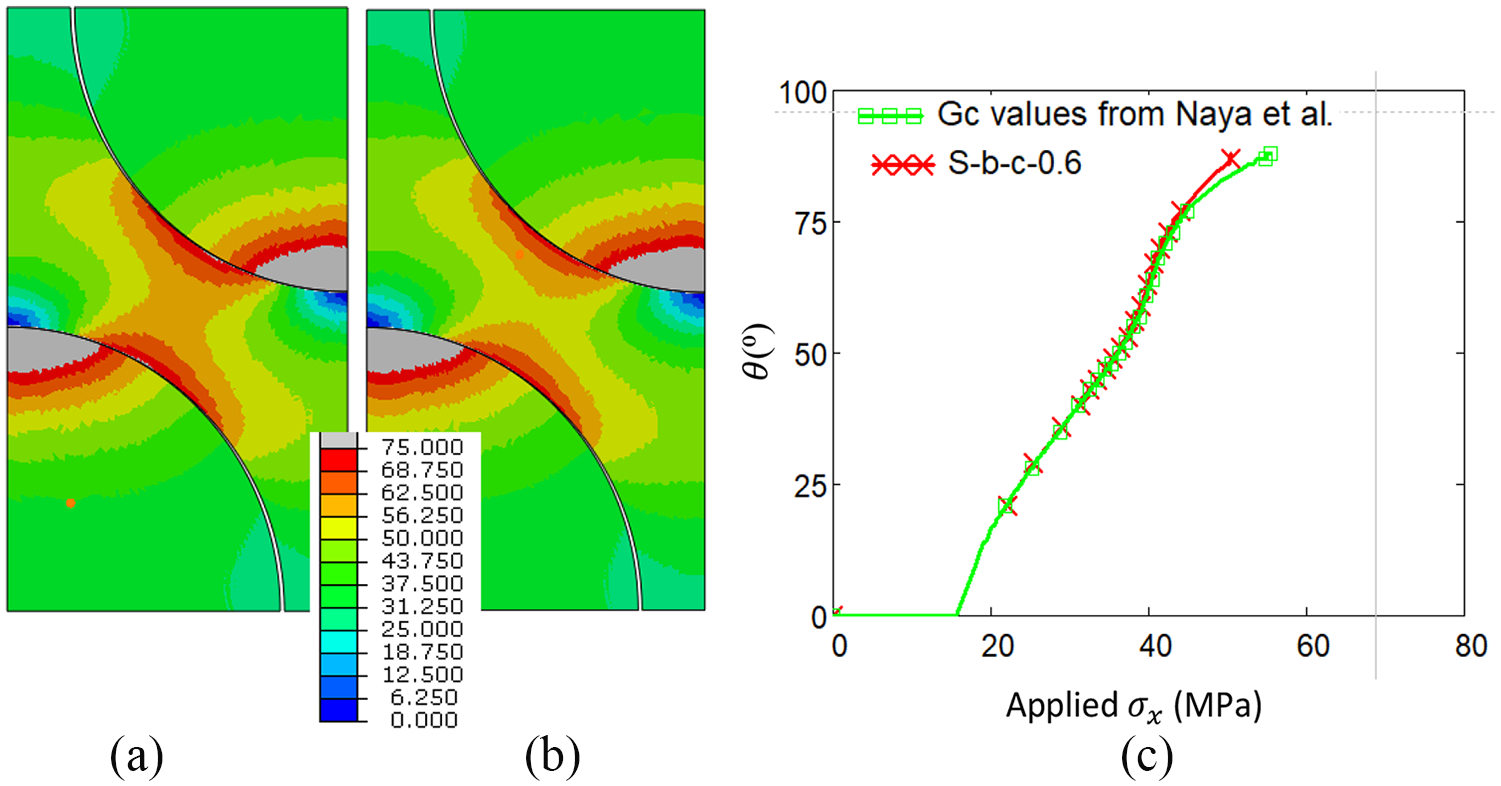
Interface-related graphical results are presented in Figure 8 with respect to the applied stress in each load step. In this figure, $N m o d$ represents the maximum normalized opening distance (the normalized distance between the nodes of the fiber and matrix at y = 0 position—shown in Figure 8(a)) and $C P R E S S$ represents the contact pressure at the bottom node. As the traction force is in the direction of separation, pressure is given as negative values. The angle, $θ$ , in Figure 8(c) is the angle of separation shown in the same figure. Untreated steel gives the maximum opening distance at the same applied stress levels compared to the other fiber types. Low adhesion strength combined with high stress concentrations results in such behavior. The importance of treating the steel fiber is shown as it gives significantly stronger behavior compared to the other fiber types.

Figure 8.

(a) $N m o d$ ; (b) $C P R E S S$ ; (c) $θ,$ ; (d) maximum of maximum principal stress in the matrix ( $S 1_{m a x}$ ) vs. applied stress for various types of models.

The vertical lines in Figure 8(c) indicate that the applied stress value for the model results in the same color when failure in the matrix is expected (maximum principal stress in the matrix reaches $S_{u t s} = 75 MPa$ ). Up to this point, fiber/matrix debonding is expected. After that point, a crack can occur and grow toward the inner regions of the matrix. The indicates that in the case of untreated steel, almost all the matrix is debonded from the fiber until failure in the matrix is expected as the opening angle values reach about 75° before $S_{u t s}$ is reached. With the plated steel, strong interface allows a separation of only 14° after which a rupture of the bulk matrix is expected. Carbon and glass results lie somewhere in between these two extremes.

Failure in the matrix is expected around 43 MPa for untreated steel fiber composite, whereas it reaches around 40 MPa for treated steel. This is an adverse effect of having a strong interface. When debonding starts, the stresses in the matrix at the debonded region are relieved as a free motion occurs at that part of the matrix. For the weak interfaces, as the separation point (and thus the critical region) moves around the fiber, it loses its perpendicular orientation with the applied load. With the strong interface, the separation point is more oriented with the applied load. The strong interface causes the matrix to carry the load, causing high stresses

In Figure 8(d), the evolution of maximum principal stresses is presented for all models together with the case in which fiber/matrix debonding is prevented. There is a slight decrease in the evolution of maximum principal stresses when debonding starts. This also shows the relief of stresses as soon as debonding starts. The evolution of maximum principal stress for a steel fiber model without separation is also provided to compare this behavior. The intersection of the horizontal line with the curves indicates the applied stress when the maximum principal stress $S_{u t s}$ is reached.

Analysis of fracture energy difference

In section “Modeling of damage behavior and the determination of damage parameters,” it was mentioned that the interface fracture energies for carbon–epoxy interface are found to be different than those of the glass–epoxy one, and no data were available for the steel–epoxy interface. Thus, the same values are used in the analyses for all fibers (as shown in Table 2). A model is constructed with fracture energy ( $G c$ ) values of carbon–epoxy interface mentioned in Naya et al.¹² and all the other properties being the same as S-b-c-0.6 to see whether this assumption causes a significant difference. The distribution of maximum principal stresses is shown in Figure 9(a). In Figure 9(b), the crack opening angle ( $θ$ ) is shown for both models. Apparently, using Gc values of carbon did not change the result significantly, even though they are more than double the one for glass. This shows that the debonding behavior is not so sensitive to the fracture energy as long as the fracture energy is kept at this grade.

Figure 9.

Maximum principal stress distribution at $σ_{x} = 43 M P a$ for the models: (a) S-b-c-0.6, (b) S-b-c-0.6 with Gc values taken from Naya et al.,¹² and (c) $θ$ vs applied $σ_{x}$ distribution for both models.

Effect of stress concentrations

In the simulations with different fibers, more than one parameter changes, making it difficult to comment on the effect of parameters. For example, more debonding is observed in blank steel fiber, and this can easily be attributed to the low adhesion strength compared to the other fiber types. However, it is known that the stress concentrations are also higher in steel fibers.⁴ So “which of these were more influential?” remains a question.

To clarify this situation, the stress concentrations and the interface strengths of two different fiber types are analyzed and the debonding angle is compared. The results from steel fiber did not reveal this effect clearly, so the comparison is performed with carbon and glass fibers (Table 4). In terms of normal stress concentrations, glass fiber composite has the higher value, so carbon fiber composite should be stronger. In terms of adhesion strength, glass fiber has the higher value and it should be stronger. When the debonding angle is checked, glass is stronger. Thus, we can conclude that the influence of adhesion strength is larger than the stress concentrations.

Table 4.

The effect of stress concentrations and adhesion strength on fiber/matrix debonding angle.

Fiber type	Maximum $K r$	$N m a x$ (MPa)	$\frac{K r_{g}}{K r_{c}}$	$\frac{N_{\max g}}{N_{\max c}}$	$θ °$ (40 MPa)
Glass	1.613	50	1.22 (carbon is stronger)	1.19 (glass is stronger)	25
Carbon	1.325	42	1.22 (carbon is stronger)	1.19 (glass is stronger)	30

$K r,$ maximum stress concentration in radial direction under transverse loading (see Sabuncuoglu et al.⁴); $g,$ glass fiber; $c,$ carbon fiber.

Effect of fiber size

To investigate and analyze the potential effect of fiber size, an additional model is generated. In this model, the blank steel fiber is modeled with the size of a glass fiber (d_f = 10 µm) instead of the original one (d_f = 30 µm) with all the other properties the same as the model S-b-c-0.6 (designated as S-b-c-0.6_with glass size). The results are shown in Figure 10. The RVE of the models was scaled according to the diameter of the fiber. Thus, in the new model, smaller RVE was used. In order to apply the same stress to this new model, the applied force was also reduced. Thus, no significant difference was observed in the debonding behavior between these two models.

Figure 10.

Maximum principal stress distribution at $σ_{x} = 43 M P a$ for the models: (a) S-b-c-0.6, (b) S-b-c-0.6_with glass size, and (c) $θ$ vs applied $σ_{x}$ distribution for both models.

Effect of fiber shape

Steel fibers are produced with polygonal cross-sectional shape due to the manufacturing process as mentioned in section “Introduction.” The fibers modeled with hexagonal cross-sectional area are compared with the circular ones to understand the effect of shape on the debonding behavior. The blank and surface-treated fibers are investigated. In our previous work, high stress concentrations were observed in hexagonal fibers.⁴ Shown in Figure 11, this also affects the debonding behavior as the debonding in polygonal fibers takes place earlier than the fibers having circular cross-sections. As it is seen in Figure 11(b), debonding along one side evolves very rapidly when the crack reaches the straight side of the hexagon. Later, it slows down at the edge, parallel to the load application direction as the crack cannot evolve easily in this direction. This also gives the indication that the orientation of the fiber cross-section relative to the loading direction is important. The distribution of maximum principal stresses at an applied stress of 30.4 MPa is presented in Figure 12 for the fibers with both cross-sectional types. Clearly, much more opening is observed in the model with hexagonal fibers compared with the circular one. A large gray area in the matrix indicates that a failure in the matrix is expected, whereas in the model with circular fibers it still remains intact at the same applied stress level. Along the straight sides of the fiber cross-section, there are some stress fluctuations. This is attributed to the numerical instabilities after a sudden debonding of the entire side of the hexagon. This is observed for only the elements on the edge of the fiber, so it does not affect the overall behavior.

Figure 11.

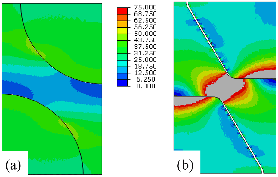
(a) Opening angle $(θ)$ and (b) $N m o d$ vs applied $σ_{x}$ for the models with hexagonal and circular fibers.

Figure 12.

Distribution of maximum principal stresses for models: (a) S-t-c-0.6 and (b) S-t-h-0.6 at an applied transverse stress of 30.4 MPa.

Effect of fiber orientation

In the previous section, the debonding behavior of hexagonal fibers was investigated in the case of a certain orientation. In that orientation, the corner fillets of the hexagon were aligned with each other, generating the minimum possible distance between the corresponding fillets of the fibers. Thus, that orientation gave more severe results in terms of debonding compared to the circular counterpart. This may be attributed to not only the polygonal cross-section but also the minimized distance between the closest points of the fibers. A question may arise here: “What if the fibers were oriented in a different way so that the distance between them is even greater than the case with circular fibers?” In order to analyze this, a model is generated by aligning the sides of the hexagon instead of the corners (Figure 13), with the other properties the same as S-b-h-0.6 (named as S-b-h-0.6-rot). The opening angle versus the applied stresses are shown in Figure 13(c). As expected, the debonding starts later than the S-b-h-0.6 due to the existence of more matrix material between the fibers. However, still debonding started earlier than the case with circular fibers, revealing that the polygonal shape is also responsible for this behavior. The amount of debonding is expected to be between these two orientation extremes in a real case where fibers are oriented randomly. Sudden debonding behavior similar to S-b-h-0.6 can be observed where the debonding reaches the sides of the hexagon. The distribution of maximum stresses at the instant when failure is expected in the matrix is shown in Figure 14(c) and (d). For the S-b-h-0.6-rot model, the stresses are more evenly distributed in the matrix. In the S-b-h-0.6 model, the region where the corners of the hexagons coincide, we see much more stress concentration showing that it is more prone to microscopic failure compared to the other orientation even if the critical stress state in the matrix was reached at the same stress level. We can also observe this similar behavior in the distribution of stresses in the fibers of both models

Figure 13.

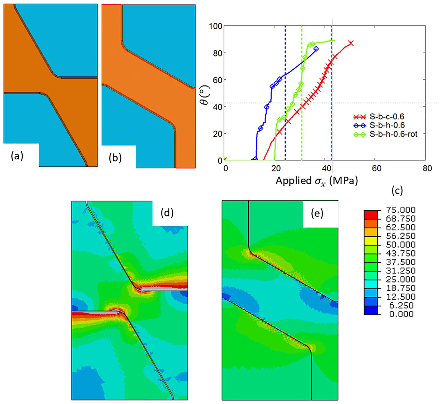
(a) S-b-h-0.6 model, (b) S-b-h-0.6-rot model, and (c) opening angle $(θ)$ vs applied $σ_{x}$ for S-b-c-0.6, S-b-h-0.6, and S-b-h-0.6-rot. Maximum principal stress distribution at the expected failure state for (d) S-b-h-0.6 model ( $σ_{x} = 24.4 M P a$ ) and (e) S-b-h-0.6-rot model ( $σ_{x} = 30.8 M P a$ ).

Figure 14.

$θ$ vs applied transverse stress for fibers with (a) circular and (b) hexagonal cross-sections. $N m o d$ vs applied transverse stress for fibers with (c) circular and (d) hexagonal cross-sections.

Effect of fiber volume fraction

Finally, fiber volume fraction is varied to observe the difference. Results are presented for both hexagonal and circular steel fibers and for vf = 0.4 and 0.6 (Figure 14). Clear observation is that for both cross-sections, the opening angle does not change with fiber volume fraction. However, $N m o d$ is significantly lower for the case vf = 0.4.

Conclusion

In this study, the debonding behavior of steel fibers was analyzed with a parametric finite element code at micro-scale. Cohesive surfaces were defined on the fiber–matrix interface to implement debonding. Interface properties of steel fibers were determined from the results of dolly tests performed for steel fibers with and without surface treatment. The results reveal the effect of main characteristics of steel fiber composites, which are the high stress concentrations and non-circular shape of the fibers. It was shown that stress concentrations have a rather weak effect on the debonding behavior compared to the interface strength. An earlier, sudden, unstable debonding behavior is expected along the straight sides if the cross-section of the fibers is not in circular shape. The improvement of surfaces of steel fibers significantly reduces the fiber/matrix debonding. With the application of treatment, the debonding behavior of these fibers can perform better than carbon and glass fibers. It is important to note that the results presented in this study are limited with the assumptions and parameters used. Especially, the parameters, such as interface strength and fracture toughness, determined in various studies show great scatter in the literature for the same fiber and matrix type. Thus, the results should be evaluated qualitatively rather than quantitatively. More detailed analyses should be performed to fully characterize the cohesive interface parameters by performing fiber push-in test for the values of fracture energy and shear strength. Some of the additional outcomes of this work are itemized below:

Fiber size does not affect the debonding behavior under the same applied stress.

The amount of debonding is not very sensitive to the fracture energy of the interface.

The debonding behavior can change depending on the amount of matrix material between the fibers due to different fiber orientations.

Fiber volume ratio affects the opening distance but not the opening angle, significantly.

In addition to the parameters studied, the effect of different fracture energies and the traction-separation law can give interesting results. However, the information about their values for different fiber–matrix interfaces is limited in the literature and suggested to be performed in the light of some experimental work. Analyzing the behavior using a different matrix type would also help the selection of the matrix type considering fiber/matrix debonding. The study can also be extended by the crack formation and growth in matrix region. As observed, after some fiber/matrix debonding, the stresses in matrix increase to extreme levels, suggesting a crack formation and growth through the matrix and joining of the fibers.

Footnotes

Data availability

The raw/processed data required to reproduce these findings can be obtained from the corresponding author upon request.

Declaration of conflicting interests

The author(s) declared no potential conflicts of interest with respect to the research, authorship, and/or publication of this article.

Funding

The author(s) disclosed receipt of the following financial support for the research, authorship, and/or publication of this article: The work reported here was funded by SIM and IWT (Flanders) in the framework of NANOFORCE program (MLM project) and The Scientific and Research Council of Turkey, project number 115C082. S.V. Lomov holds Toray Chair for Composite Materials at KU Leuven, support of which is acknowledged.

ORCID iD

Baris Sabuncuoglu

References

Callens

Gorbatikh

Verpoest

Ductile steel fibre composites with brittle and ductile matrices. Compos Part A: Appl S 2014; 61: 235–244.

Callens

De Cuyper

Gorbatikh

, et al. Effect of fibre architecture on the tensile and impact behaviour of ductile stainless steel fibre polypropylene composites. Compos Struct 2015; 119: 528–533.

Callens

Gorbatikh

Bertels

, et al. Tensile behaviour of stainless steel fibre/epoxy composites with modified adhesion. Compos Part A: Appl S 2015; 69: 208–218.

Sabuncuoglu

Orlova

Gorbatikh

, et al. Micro-scale finite element analysis of stress concentrations in steel fiber composites under transverse loading. J Compos Mater 2014; 49: 1057–1069.

Tsai

SW.

Theory of composites design. Dayton, OH: Think Composites, 1992.

Degrieck

Van Paepegem

Fatigue damage modeling of fibre-reinforced composite materials: review. Appl Mech Rev 2001; 54: 279–300.

Maligno

Warrior

Long

AC.

Effects of inter-fibre spacing on damage evolution in unidirectional (UD) fibre-reinforced composites. Eur J Mech A: Solid 2009; 28: 768–776.

Ghosh

Ling

Majumdar

, et al. Interfacial debonding analysis in multiple fiber reinforced composites. Mech Mater 2000; 32: 561–591.

Canal

Segurado

Llorca

Failure surface of epoxy-modified fiber-reinforced composites under transverse tension and out-of-plane shear. Int J Solids Struct 2009; 46: 2265–2274.

10.

García

Hart

Wardle

BL.

Long carbon nanotubes grown on the surface of fibers for hybrid composites. AIAA J 2008; 46: 1405–1412.

11.

Mora

González

Lopes

, et al. Analysis of transverse cracking in unidirectional composite plies by means of computational micromechanics. In: 16th European conference on composite materials, Seville, 22–26 June 2014.

12.

Naya

González

Lopes

, et al. Combined multi-scale simulations in fiber-reinforced composites. In: 16th European conference on composite materials, Seville, 22–26 June 2014.

13.

Wood

Bradley

WL.

Determination of the effect of seawater on the interfacial strength of an interlayer E-glass/graphite/epoxy composite by in situ observation of transverse cracking in an environmental SEM. Compos Sci Technol 1997; 57: 1033–1043.

14.

Suresh

Raghavendra

Anjanappa Venkataswamy

, et al. Fractographic analysis of tensile failures of aerospace grade composites. Mater Res 2012; 15(6): 990–997.

15.

De Bondt

Decrop

. Bundle drawn stainless steel fibers. United States Patent 7166174, 2007.

16.

Kushch

Shmegera

Mishnaevsky

Jr . Explicit modeling the progressive interface damage in fibrous composite: analytical vs. numerical approach. Compos Sci Technol 2011; 71: 989–997.

17.

Maligno

Warrior

Long

AC.

Effects of interphase material properties in unidirectional fibre reinforced composites. Compos Sci Technol 2010; 70: 36–44.

18.

Tang

Hammi

Horstemeyer

, et al. Finite element micromechanical analysis of the deformation and stress state dependent damage evolution in fiber reinforced metal matrix composites. Comp Mater Sci 2012; 59: 165–173.

19.

Banerjee

Sankar

BV.

Mechanical properties of hybrid composites using finite element method based micromechanics. Compos Part B: Eng 2014; 58: 318–327.

20.

Sun

Vaidya

Prediction of composite properties from a representative volume element. Compos Sci Technol 1996; 56: 171–179.

21.

Okabe

Ishii

Nishikawa

, et al. Prediction of Tensile Strength of Unidirectional CFRP Composites. Adv Compos Mater 2010; 19: 229–241.

22.

Turon

Dávila

Camanho

, et al. An engineering solution for mesh size effects in the simulation of delamination using cohesive zone models. Eng Fract Mech 2007; 74: 1665–1682.

23.

Simulia

. Abaqus version 2016 documentation USA. Johnston, RI: Dassault Systems Simulia Corp, 2016.

24.

Song

Davila

Rose

. Guidelines and parameter selection for the simulation of progressive delamination, https://ntrs.nasa.gov/archive/nasa/casi.ntrs.nasa.gov/20080020385.pdf

25.

Ghosh

Bertels

Goderis

, et al. Optimisation of wet chemical silane deposition to improve the interfacial strength of stainless steel/epoxy. Appl Surf Sci 2015; 324: 134–142.

26.

Bhattacharya

Siegmund

The role of glottal surface adhesion on vocal folds biomechanics. Biomech Model Mechan 2015; 14: 283–295.

27.

Thouless

Waas

, et al. Use of a cohesive-zone model to analyze the fracture of a fiber-reinforced polymer–matrix composite. Compos Sci Technol 2005; 65: 537–549.

28.

Cai

Study on the interfacial strength of steel fibre polymer composites. Leuven: KU Leuven, 2012.

29.

Wang

, et al. An improved microbond test method for determination of the interfacial shear strength between carbon fibers and epoxy resin. Polym Test 2013; 32: 1460–1465.

30.

Choi

N-S

Park

J-E.

Fiber/matrix interfacial shear strength measured by a quasi-disk microbond specimen. Compos Sci Technol 2009; 69: 1615–1622.

31.

Ogihara

Koyanagi

Investigation of combined stress state failure criterion for glass fiber/epoxy interface by the cruciform specimen method. Compos Sci Technol 2010; 70: 143–150.

32.

Kanchanomai

Rattananon

Soni

Effects of loading rate on fracture behavior and mechanism of thermoset epoxy resin. Polym Test 2005; 24: 886–892.

Micro-scale numerical study of fiber/matrix debonding in steel fiber composites

Abstract

Keywords

Introduction

Micromechanical model

Modeling of damage behavior and the determination of damage parameters

Verification of the numerical model

Determination of the viscous regularization coefficient

Verification of the mesh structure

Verification of the cohesive zone application

Results

Comparison of steel fibers with glass and carbon fibers

Analysis of fracture energy difference

Effect of stress concentrations

Effect of fiber size

Effect of fiber shape

Effect of fiber orientation

Effect of fiber volume fraction

Conclusion

Footnotes

Data availability

Declaration of conflicting interests

Funding

ORCID iD

References