Sage Journals: Discover world-class research

Abstract

Although textile production is heavily automation-based, it is viewed as a virgin area with regard to Industry 4.0. When the developments are integrated into the textile sector, efficiency is expected to increase. When data mining and machine learning studies are examined in textile sector, it is seen that there is a lack of data sharing related to production process in enterprises because of commercial concerns and confidentiality. In this study, a method is presented about how to simulate a production process and how to make regression from the time series data with machine learning. The simulation has been prepared for the annual production plan, and the corresponding faults based on the information received from textile glove enterprise and production data have been obtained. Data set has been applied to various machine learning methods within the scope of supervised learning to compare the learning performances. The errors that occur in the production process have been created using random parameters in the simulation. In order to verify the hypothesis that the errors may be forecast, various machine learning algorithms have been trained using data set in the form of time series. The variable showing the number of faulty products could be forecast very successfully. When forecasting the faulty product parameter, the random forest algorithm has demonstrated the highest success. As these error values have given high accuracy even in a simulation that works with uniformly distributed random parameters, highly accurate forecasts can be made in real-life applications as well.

Keywords

Textile glove fault forecasting time series artificial intelligence simulation machine learning

Introduction

Considered as having started with the introduction of cyber-physical systems, Industry 4.0 has now begun to change the way industrial organizations operate. Technologies such as artificial intelligence (AI), additive manufacturing, Internet of things, augmented reality, smart robotic systems, big data, and cloud computing support the efficiency and speed of many industrial processes such as production, planning, R&D, quality management, supply, order, and so on. Looking at where each sector is with regard to the application of Industry 4.0 technologies or the transformation process of businesses, it can be seen in various studies that defense, health, automotive, and white goods industries have progressed to more advanced levels than textile, leather, food, and furniture.^1–3 Although textile production is heavily automation-based, it is viewed as a virgin area with regard to Industry 4.0 technologies. When the developments in informatics are integrated into the textile sector, efficiency is expected to increase by way of higher productivity, lower costs, shorter processes, and fewer faults.⁴

The basic workflow in the textile sector is given in Figure 1. Accordingly, production is done in line with the planning process based on the orders received and the designs made. The product obtained at the end of the production is delivered if it meets the order criteria. However, the production process and the product must be constantly inspected by the quality control process, and any faults must be corrected and replanned. Among these steps, design, planning, production, and quality control processes are specific to the textile sector, whereas order and delivery processes are of interest for the other sectors. Forecasts in the textile sector cover the use of various methods to correct the faults that occur in design, production, and products in order to improve the quality control processes.

Figure 1.

Production flowchart in textile industry.

Design in textile involves drawing and developing patterns, textures, molds, and products in line with customer demands and expectations. During the design process, the tasks are done either by computer or by drawing manually and depend on the designer’s artistic ability. Therefore, it is hard to express the design process using a mathematical equation. The product model obtained at the end of the design process must be adapted to different body sizes before mass production starts. Hu et al.⁵ used artificial neural networks for predicting the suitable body size for the novice designers making a design using the design experience. In making design, Hsu and Wang⁶ reviewed the issue of sizing in the production of clothing. In their study, they used the decision tree (DT) method for the production of clothing.

Production covers all the textile processes, from order receipt to manufacturing the product to be delivered to the customer. Throughout this process, the standard information that the business owns is the nature of the order and the raw material quality. But the period of time, the raw materials and the processes required to produce the desired product depend on the quantity and quality of personnel and machinery available in the company. Raw material goes through many processes including dyeing, coating, thermal processes, washing, sewing, cutting, and so on until the end product is obtained. These processes include many parameters within themselves. Doing production with so many parameters requires specialized personnel, experience, and care. Highly faulty production is unavoidable in human-dependent systems. Doing planning so that the desired product is obtained by production planning operations is both very important in reducing the cost and the number of faults and is a very difficult field that requires expertise. Looking at the machine learning (ML) studies performed in this field, it has been seen that there is work done in relation to yarn finish operations,⁷ fabric finish operations,⁸ discriminating product colors,^9,10 and export forecasts.¹¹

Yarn quality determination is a process where parameters such as strength, hairiness, breaking elongation, and production errors are inspected by means of control and measurement. This process is commonly conducted using the Tester device of the USTER company. This device is costly and therefore hardly available for small-scale companies. To reduce the quality measurement cost of businesses, Mozafary and Payvandy¹² have used artificial neural network method to predict the worsted yarn quality. Yildiz et al.¹³ have made breaking elongation and sewing strength modeling for yarns by using the artificial neural network method. Haghighat et al.¹⁴ have used artificial neural networks in forecasting the hairiness of polyester-viscose blended yarns. Su and Lu¹⁵ have used artificial neural networks in determining spandex faults. Lewandowski and Stanczyk¹⁶ have used artificial neural networks to determine the yarn splices. Nurwaha and Wang¹⁷ have used artificial neural networks and support vector machine (SVM) algorithm to do yarn quality forecasts. Abakar and Yu¹⁸ have used artificial neural networks and SVM algorithm to determine yarn strength.

There is still a lack of a standard device used commonly for detecting fabric faults, and determination of faults is generally done by the human eye. When quality control and fault determination in textile are done by humans, natural conditions such as fatigue or sleepiness lead to improper quality control, and therefore, there is a requirement to detect fabric faults automatically. Within the scope of visual fault perception studies in textile, various works demonstrate that conventional image processing techniques are widely used and successful results are being obtained in limited fields of application.^19–21 Such practices have become popular today, particularly because of the high performance, flexibility, and ease of application provided by ML methods in signal and image processing. Among these studies, there are various works on the determination of faults and fault types in the types of fabrics such as embroidered,²² plain weave,²³ yarn dye,²⁴ and so on. Similar methods have also been used to predict structural fabric features such as hairiness,²⁵ pilling,²⁶ stretching,²⁷ humidity, and heat transfer.²⁸

Predictions in the field of quality control in businesses had for a long time been made using statistical methods such as autoregression (AR), moving average (MA), and vector autoregression (VAR).^29,30 However, toward the end of the 1970s, it was seen that linear models are not compatible with and are inadequate for real-life applications.³¹ Non-linear time series models have also been suggested in the same process. However, these systems are also insufficient for today’s practices and are being replaced by artificial learning, also known as ML, which is a sub-branch of AI.^32,33 Time series analyses and prediction work in the textile sector have been focused more on demand forecasting.^34–37 A review of the data mining and ML applications in the textile sector demonstrates a lack of data sharing in this subject. This study aims to provide a method to forecast the possible amount of faulty products and the production period based on the production planning information that is created using the information obtained during the ordering phase. Within the scope of the problem, a simulation has been prepared for the annual production plan, and the corresponding faults based on the information received from textile glove plant and production data have been obtained. Data set has been prepared using the parameters of a real business, while respecting the confidentiality of the business and protecting the real statistical properties. In addition to the raw data set, ML has been used to do time series analysis. Data set has been applied to various ML methods within the scope of supervised learning to compare the learning performances. The model making the most accurate predictions has been presented in the results. In the following parts of this article, the method to be used, the simulation algorithm, the data set structure, and a comparison of the results obtained by ML will be presented in the given order. Finally, comes the conclusion drawn from the findings. The study is innovative for the textile sector since it can make predictions for a random process with the simulation environment and ML it provides. This is also the first time the production phases of a textile company have been simulated.

Materials and methods

Production simulation and data set properties

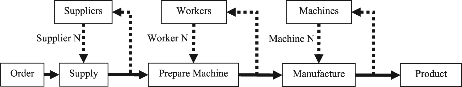
The data set to be used in the study consists of the fault log for the production process in the 1095 workdays between January 1 2017 and January 1 2020. Eleven suppliers, 7 workers, and 40 machine agents have been used for the simulation. Simulation environment has been prepared using Python programming language. Simpy mutually exclusive event simulation library has been used for time triggering of events.³⁸ Data have been created using the method shown in Figure 2 according to the multiple agent simulation of the supplier, worker, and machine components based on the data obtained from a textile company producing knitted gloves. Production plans are based on procurement in line with the orders. Procurement has different features for each product type. After procurement has been completed, a worker prepares the machine according to the production plan. Following the machine preparation phase, a unique product type is entered in each machine, which then manufactures the ordered amount of products. Faults may occur in each of the supply, prepare, and manufacture phases. Within a production plan, each supplier and worker agent has the same operating principle, and the flow diagram of these agents is given in Figure 3. First of all, the supplier, worker, and machines are selected in the product planning phase. After the selected supplier produces the raw material, the machine and worker pairs matched in the shift manufacture the products.

Figure 2.

Simulation flowchart.

Figure 3.

Supplier and worker agent algorithm.

Supplier and worker agents have been created using the same operating principle. The algorithm used for these agents is given in Figure 3. According to this algorithm, a random fault value is created in each production, and if this value is lower than the error rate threshold, then a fault occurs. After the occurrence of a fault, the situation is detected, and correction chance inspection is performed, meaning that the worker learns the work and makes fewer errors. The error rate is reduced under these conditions. Each supplier and worker agent has a unique identifier error rate, maximum error, correction rate, and working rate (WR). Error rate, correction rate, and maximum error values are the internal variables of the agent and not included in the raw data. Error rate represents the fault rate value of the agent. Correction rate is used for reducing the error rate and represents the case in which the agent gains experience in time and makes fewer errors. The error limit is the ultimate error rate, even if the error rate has been corrected. WR is the number of successful tasks of the agent divided by the total number of tasks. WR is included in raw data and is a value that can be added in the real application. Data creation was based on the assumption that the supplier and the worker error rate is between 0.05 and 0.15, the maximum error rate is between 0.01 and 0.02, and correction rate is between 0.001 and 0.002.

Machine agents have different structures from supplier and worker agents with regard to error correction and periodical error formation. The algorithm created for a machine agent is given in Figure 4. A random error formation value is created inside the machine according to this algorithm, and an error occurs if this value is lower than the value determined for the agent. Also, a periodical error value has been defined to represent the errors that may occur due to the life of the parts inside the machine. An error occurs when the period value is exceeded in terms of the number of production, then the part is considered to have been renewed, the day counter is reset and the periodic maintenance period is slightly changed randomly within the interval of 9500–10,500. Data creation was based on an assumed machine error rate between 0.02 and 0.05.

Figure 4.

Machine agent algorithm.

The simulation data created in this study include information about daily raw material, personnel, and machines in use. In the study, the sources of error in the plant have been grouped into three, such as supplier, worker, and machine errors. Supplier errors include faulty yarn number, low strength yarn, delivery of yarns in different colors, and hues. Raw material errors are also known as yarn-based errors. Examples are errors such as thick yarn, thin yarn, and yarn cutting. Worker errors include the worker’s loading wrong raw materials and making incorrect adjustments to the machine. One of the most important worker errors is the incorrect machine configuration. Incorrect adjustment of yarn frequency by the personnel leads to transverse lines in the knitted fabric. Faulty yarns and yarns with the wrong number cause faults in knitted fabric such as transverse horizontal lines at regular intervals, which look like grooves. Machine errors are power failures, sensor perception errors, and errors caused by deformation of machine parts. These errors may occur either singly or in combinations of two or three. Pictures of faulty gloves are presented in Figure 5 as an example of this condition. Figure 5(a) shows a fingertip error that has occurred as a result of worker error. Figure 5(b) is the case in which the wrist of the glove has not been produced because of the raw material. Figure 5(c) shows the error that has occurred because of the deformation in the machine needle. These errors create vertical tracks or lines in the gloves. This is caused by vertical rows that are tighter or looser than the others. Another reason is that the needle replaced with the defective one creates a source of error. Figure 5(d) is a hybrid error caused by the supplier and the worker. This is a faulty production due to yarn raw material error and incorrect loading of the machine by the personnel.

Figure 5.

Fault types: (a) worker error, (b) supplier error, (c) machine error, and (d) supplier–worker error.

In the study, ML methods have been used to forecast the amount of the possible fault and the period of completion based on the attribute parameters. The parameters used for this purpose for a supplier, worker, and machine are summarized in Table 1. The WR parameters defined for the supplier and the worker are the number of successful tasks of the supplier or the worker divided by the total number of tasks. All data have been shared as an attachment to the publication.

Table 1.

Data set properties.

Parameter	Explanation	Usage
ST	Production start time	Feature
OID	Order identification number	Feature
NO	Number of order type	Feature
AO	Amount of order	Feature
SID	Supplier identification number	Feature
SWR	Current working rate of supplier. Division of unsuccessful supplies to all supplies.	Feature
WID	Worker Identification number	Feature
WWR	Current working rate of worker. Division of unsuccessful prepares to all prepares.	Feature
MID	Machine identification number	Feature
MC	Machine manufacture counter	Feature
AF	Amount of fault	Target
ET	Elapsed time as hour	Target

ML concept and time series

AI researchers created new techniques, developed and applied them to solve engineering problems since three decades. ML is a sub-branch of AI that provides systems the ability to learn and improve from data without being explicitly programmed. ML is used especially for applications where a clear equation is not extracted from the experimental data.^39–41

Time series prediction is often defined as a supervised learning problem as the examination of the changes in time usually consists of supervisor-prepared labels/values. These types of applications are mostly used in classical signal processing applications such as fault diagnosis ^42–44 and human motion recognition.^45–47 Time series prediction can be defined as a supervised learning problem. In supervised learning, the aim is to approximate the real underlying mapping so well that when you have new input data, you can predict target variable for that data.

Supervised learning can be grouped into regression and classification problems. When the target variable is a categorical, such as “green,” “red,” and “blue,” the problem is called a classification problem. When the target variable is a continuous value, such as “temperature” or “weight,” the problem is called as regression. If you have a time series data set you can get historical information. This historical data set is usually part of the same set of time series that is defined within certain limits and prior to the current data. The restriction interval of this data set is moved over time in a certain amount of time for each processed data. Therefore, this method is called the sliding window.^33,48,49

Regression algorithms

DT

The DT algorithm is an algorithm frequently used in statistical learning and data mining. DT is an algorithm that works with simple if-then-else decision rules and is used for both classification and regression in supervised learning.⁵⁰ The DT algorithm has three basic steps. In the first step, the most meaningful feature placed as a first (root) node. In the second step, according to this node divide data set into subsets. Subsets should be made in such a way that each subset contains data with the same value for a feature. In the third step, repeat steps 1 and 2 until find last (leaf) nodes in all the branches. DT builds classification or regression models in the form of a tree structure. It splits a data set into smaller subsets while at the same time an associated DT is incrementally developed. Result of the algorithm is a tree with decision nodes. DTs can handle both categorical and numerical data.⁵¹

K nearest neighbors

The K nearest neighbors (KNN) algorithm is a learning algorithm that works according to the values of the nearest K neighbor. The KNN algorithm is a non-parametric method for classification and regression.⁵² It was first applied to the classification of news articles.⁵³ When performing learning with the KNN algorithm, first the distance of each datum to the other is calculated in the data set examined. This length calculation is done with Euclidian, Manhattan, or Hamming distance function. Then, for each data mean of nearest K neighbors is calculated. The K value is the only hyperparameter of the KNN algorithm. When deciding K value, if the K is too low, then the borders are going to be flickering and overfit situation occurs, whereas if the K value is too high, the separation borders going to be smoother and underfit situation occurs. The disadvantage of the KNN algorithm is the distance calculation process because it increases the process load as the amount of data increases.

Adaptive Boosting

The Adaptive Boosting (AdaBoost) algorithm is an ML method called a type of ensemble method. The aim of this method is to create a stronger learning structure by using weak learners. AdaBoost can be used to improve the performance of any ML algorithm. However, this method often uses a single-level DT algorithm as a weak learner algorithm, because the process load is much lower than other basic learning algorithms. The AdaBoost algorithm consists of four basic steps. In the first step, the N weak algorithms are run, and the data set is learned. Each of these N weak learning algorithms is assigned a weight value of 1/N. In the second step, the error values are calculated each learner algorithm. In the third step, the weight value of the learning algorithm with a high amount of error is increased. In the fourth step, the learning algorithms are summed with weights and if the desired metric limit is reached, the total algorithm is output else return to the second step.^54–56 As the number of learners in this algorithm increases, the process load and the learning performance increase.

Random forest

The random forest (RF) method is designed in the form of a forest consisting of many DTs. Each DT in the forest is formed by selecting the sample from the original data set with bootstrap technique and selecting the random number of all variables in each decision node. The RF algorithm consists of four fundamental steps. First of all, randomly select n features from total m features. For the second step, among the n features, calculate the node d using the best split point. In the third step, check whether the number of final (leaf) nodes reached to target if it is not go to step 1 otherwise go to next step. For the last step, build forest by repeating steps 1–3 for n (number of trees in forest) times.^57–59

SVM

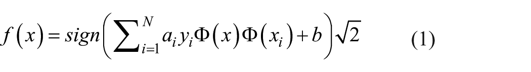
SVM was first introduced by Vapnik.⁶⁰ SVM is a frequently used ML method for classification and regression problems. SVMs used for classification are called support vector classifier (SVC), and SVMs used for regression are called support vector regressor (SVR). The SVM is mainly divided into two according to the linear separability of the data set. Non-linear SVM decision function is given in equation (1). In cases where the data cannot be separated linearly, the data are moved to a space of higher dimension, and kernel functions (KFs) are used to resolve them. The transformations can be made by using KFs expressed as K(x_i, x_j) = Φ(x) Φ(x_i) instead of Φ(x) Φ(x_i) scalar product given in equation (1). Non-linear transformations can be made, and the data can be separated in the high dimension thanks to the KFs. Therefore, KFs have a critical role in the performance of SVM. The most commonly used KFs are presented in Table 2.^61,62 The performance of SVM model varies according to penalty cost (C), insensitivity zone (ε), KF type, and function coefficients. C determines the trade-off between the training error and dimension of the model. A small value for C will increase the number of training errors, while a large C will lead to behavior similar to that of a hard margin SVM. The ε value affects the width of the intensive zone of vectors. As the value of ε increases, the number of support vectors decreases and provides a smoother estimation.^63,64 Commonly used KF are linear, polynomial, sigmoid, and radial basis (RB). The RB function is the most popular choice because of their localized and finite responses

f (x) = s i g n (\sum_{i = 1}^{N} a_{i} y_{i} Φ (x) Φ (x_{i}) + b) \sqrt{2}

(1)

Table 2.

SVM kernel functions.

Kernel function	Formulation
Linear	$K (x_{i}, x_{j}) = (x_{i}^{T} x_{j})$
Polynomial	$K (x_{i}, x_{j}) = {(x_{i} x_{j})}^{d}$
Radial basis function (RBF)	$K (x_{i}, x_{j}) = \exp (- γ {‖ x_{i} - x_{j} ‖}^{2}), γ > 0$
Sigmoid	$K (x_{i}, x_{j}) = \tan h (k x_{i} x_{j} - δ)$

Performance evaluation and model selection

There are a number of model evaluation techniques but some of the most well-known are percentage split and cross-validation. In the evaluation processes, it is essential to use a train and a test data set. Percentage split is the most basic method. In this method, all the data are split as train and test manually. Training data sets are used for learning process, and test data set is used for performance evaluation. However, evaluation results may not be reliable because of the reasons such as not having the same distribution when selecting the train and test data in the data set, uneven distribution of outliers, and so on. Therefore, cross-validation method has been developed. In this method, train and test data are integrated and turned into a single data set. All data are divided into K equal-sized subsets. The K value which is also called as fold number is determined by the user. Then, learning and testing are performed for each of the K subsets; here one of the subsets will be test, and the other will be train. As a result, performance metrics are obtained for each subset. The average of the performance metrics is considered as the performance metric of the K-fold cross-validation. The K-fold cross-validation method is known to produce more reliable results than other methods. 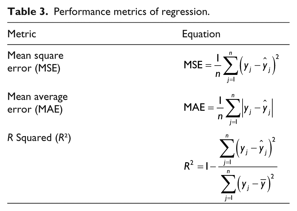However, since learning and testing for each subset are performed separately for all subsets, the total time spent is longer than the other methods.⁴¹ The main criteria used for performance evaluation and model selection are called metrics. The most commonly used regression metrics are mean square error (MSE), mean average error (MAE), and coefficient of determination (R²). The MSE, MAE, and R² metrics used in the regression performance evaluation are given in Table 3.^41,65,66 For the equations in Table 3, ${\hat{y}}_{j}$ is the predicted value and $y_{j}$ is the observed value.

Table 3.

Performance metrics of regression.

Metric	Equation
Mean square error (MSE)	$MSE = \frac{1}{n} \sum_{j = 1}^{n} {(y_{j} - {\hat{y}}_{j})}^{2}$
Mean average error (MAE)	$MAE = \frac{1}{n} \sum_{j = 1}^{n} \| y_{j} - {\hat{y}}_{j} \|$
R Squared (R²)	$R^{2} = 1 - \frac{\sum_{j = 1}^{n} {(y_{j} - {\hat{y}}_{j})}^{2}}{\sum_{j = 1}^{n} {(y_{j} - \bar{y})}^{2}}$

Results and discussion

Simulation results

Simulation environment has been prepared using Python programming language. Simpy mutually exclusive event simulation library has been used for time triggering of events. Eleven suppliers, 7 workers, and 40 machines have been used as simulation assets according to the data received from the plant. The data of the simulation is shared in the supplementary materials. The simulation was based on 6 workdays and 24 h throughout the 1095 workdays in the interval of 2017–2020. The average production value per order has been uniformly assigned in increments of 50 between 100 and 900. A glove is produced in about 3–6 min. Procurement takes about 1–10 h, depending on the type of order. It takes about 30–60 min for the worker to make production adjustments for each device. The initial error values of the suppliers and the workers are assigned randomly in the interval of 0.05 and 0.15. These values are then reduced as errors occur but do not fall below the limit value of 0.02. The value 0.02 has been identified as the minimum error value in operation. The machine error rate has been randomly assigned in the interval of 0.02 and 0.05. The core value for creating random value for the repeatability of simulation has been chosen as 2. A total of 1570 orders have been created as a result of the simulation. In the simulation process, the cases in which the rate of faulty production is more than 2% of the production have been marked as faulty production. The results obtained by using the Pearson method to calculate the absolute cross-correlation values of the variables according to the simulation results are presented in Figure 6. This figure shows the relations of input and output variables and those with low relations approach to 0 and those with high relationship to 1. Accordingly, the output value AF is mostly correlated with the AO variable, and the value is 0.79. The correlation of AF with the other variables is less than 0.1. The ET output variable is mostly correlated with the AO and SID variables. But these variables have a weak correlation.

Figure 6.

Absolute cross-correlation map of variables.

Amount of fault prediction

The ML methods mentioned in section “Materials and methods” are used for forecasting the AF value. The performance evaluation results obtained by 10-fold cross-validation at the end of training with these algorithms are given in Table 4. Training time, MSE, MAE, and R² results are presented in Figure 7 in box drawing, showing the distribution and the median. As for training time, the KNN algorithm has been the algorithm that has completed the training process in the shortest time with 0.00158 s on the average. According to the available results, the RF algorithm has been the most successful algorithm for all three parameters. The application of test values to the RF algorithm for validation, and the resulting forecasts are shown in Figure 8. This figure shows the predicted and actual values, and in the case of regression, if the predicted and actual values overlap exactly, the offset value is 0 and is expected to occur with a slope of 45°. As a result of the validation test with the RF algorithm, the MSE value has been calculated as 26.185. The linear equation obtained by linear regression between prediction and validation values is y = 0.73x + 4.29.

Table 4.

Amount of fault prediction mean values of training time and performance metrics.

ML algorithm	Training time	MSE	MAE	R ²
DT	0.00739	54.681	5.495	0.485
KNN	0.00158	51.107	5.426	0.525
AdaBoost	0.08790	38.000	4.846	0.646
RF	0.04230	31.918	4.289	0.702
SVR	0.04875	44.394	4.894	0.588

ML: machine learning; MSE: mean square error; MAE: mean average error; DT: decision tree; KNN: K nearest neighbors; AdaBoost, Adaptive Boosting; RF: random forest; SVR: support vector regressor.

Figure 7.

Training time and performance metrics of fault amount prediction.

Figure 8.

Validation of RF in fault amount prediction.

Elapsed time prediction

The ML methods mentioned in section “Materials and methods” are used for forecasting the ET value. The performance evaluation results obtained by 10-fold cross-validation at the end of training with these algorithms are given in Table 5. MSE, MAE, and R² results are presented in Figure 9 in box drawing, showing the distribution and the median. As for training time, the KNN algorithm has been the algorithm that has completed the training process in the shortest time with 0.00163 s on the average. According to the available results, the SVR algorithm has been the most successful algorithm for all three parameters. The application of test values to the SVR algorithm for validation and the resulting forecasts is shown in Figure 10. As a result of the validation test with SVR algorithm, the MSE value has been calculated as 80.731. The linear equation obtained by linear regression between prediction and validation values is y = 0.15x + 12.19.

Table 5.

Elapsed time prediction mean values of training time and performance metrics.

ML algorithm	Training time	MSE	MAE	R ²
DT	0.00828	131.392	5.494	−0.518
KNN	0.00163	87.665	5.414	0.025
AdaBoost	0.02434	84.881	6.339	0.080
RF	0.04920	76.645	4.695	0.124
SVR	0.05325	75.829	3.909	0.192

ML: machine learning; MSE: mean square error; MAE: mean average error; DT: decision tree; KNN: K nearest neighbors; AdaBoost, Adaptive Boosting; RF: random forest; SVR: support vector regressor.

Figure 9.

Training time and performance metrics of elapsed time prediction.

Figure 10.

Validation of SVR in elapsed time prediction.

Conclusion

For the purpose of the study, since data cannot be obtained from businesses because of commercial concerns and confidentiality, the data related to the production process have been created by way of simulation based on production parameters of a glove manufacturer. The errors that occur in the production process have been created using random parameters in the simulation. In order to verify the hypothesis that the errors may be forecast, various ML algorithms have been trained using data set in the form of time series. At the end of the study, because of the possible failures in the production process, the ET variable representing the completion time of the order could not be forecast successfully. However, the AF variable showing the number of faulty products could be forecast very successfully. When forecasting the AF parameter, the RF learning algorithm has demonstrated the biggest success with 31.918 MSE value in the training phase and 26.185 MSE value in the testing phase. As these MSE values have given high accuracy even in a simulation that works with uniformly distributed random parameters, highly accurate forecasts can be made in real-life applications as well.

Supplemental Material

fsim_data_1 – Supplemental material for Production fault simulation and forecasting from time series data with machine learning in glove textile industry

Supplemental material, fsim_data_1 for Production fault simulation and forecasting from time series data with machine learning in glove textile industry by Mine Seçkin, Ahmet Çağdaş Seçkin and Aysun Coşkun in Journal of Engineered Fibers and Fabrics

Footnotes

Acknowledgements

The authors would like to thank UŞELSAN Textile Products Company and the owner Ümit Özkır for the information provided for the study.

Declaration of conflicting interests

The author(s) declared no potential conflicts of interest with respect to the research, authorship, and/or publication of this article.

Funding

The author(s) received no financial support for the research, authorship, and/or publication of this article.

ORCID iDs

Mine Seçkin

Ahmet Çağdaş Seçkin

Supplemental material

Supplemental material for this article is available online.

References

Rüßmann

Lorenz

Gerbert

, et al. Industry 4.0: the future of productivity and growth in manufacturing industries. Boston Consult Group 2015; 9: 54–89.

TÜSİAD. Industry 4.0 in Turkey as an imperative for global competitiveness—an emerging market perspective, 2016, https://tusiad.org/en/reports/item/9011-industry-40-in-turkey-as-an-imperative-for-global-competitiveness

Yüksel

Sener

The reflections of digitalization at organizational level: industry 4.0 in Turkey. J Bus Econ Finance 2017; 6: 291–300.

Yildirim

Birant

Alpyildiz

Data mining and machine learning in textile industry: data mining in textile industry. Wiley Interdiscip Rev Data Min Knowl Discov 2018; 8: e1228.

Z-H

Ding

Y-S

X-K

, et al. A hybrid neural network and immune algorithm approach for fit garment design. Text Res J 2009; 79: 1319–1330.

Hsu

C-H

Wang

M-JJ

. Using decision tree-based data mining to establish a sizing system for the manufacture of garments. Int J Adv Manuf Technol 2005; 26: 669–674.

Akyol

Tüfekci

Kahveci

, et al. A model for predicting drying time period of wool yarn bobbins using computational intelligence techniques. Text Res J 2015; 85: 1367–1380.

Kursun

Kalaoğlu

Jevšnik

, et al. Use of artificial neural networks for modelling the drape behaviour of woollen fabrics treated with dry finishing processes. Fibres Text East Eur 2015; 2(110): 90–99, http://yadda.icm.edu.pl/baztech/element/bwmeta1.element.baztech-0b7b71b6-59cd-4c44-abf8-3d2e4e8c8baa (accessed 3 February 2019).

Zhang

Yang

Evaluation model of color difference for dyed fabrics based on the support vector machine. Text Res J 2014; 84: 2184–2197.

10.

Furferi

Governi

Volpe

Modelling and simulation of an innovative fabric coating process using artificial neural networks. Text Res J 2012; 82: 1282–1294, https://journals.sagepub.com/doi/abs/10.1177/0040517512436828 (accessed 3 February 2019).

11.

Ozbek

Akalin

Topuz

, et al. Prediction of Turkey’s denim trousers export using artificial neural networks and the autoregressive integrated moving average model. Fibres Text East Eur 2011; 19: 10–16.

12.

Mozafary

Payvandy

Application of data mining technique in predicting worsted spun yarn quality. J Text Inst 2014; 105: 100–108.

13.

Yildiz

Dal

Ünal

, et al. Use of artificial neural networks for modelling of seam strength and elongation at break. Fibres Text East Eur 2013; 5(101): 117–123, http://yadda.icm.edu.pl/baztech/element/bwmeta1.element.baztech-fd9e2e37-ef8a-455f-b14c-1deb6e8435e2 (accessed 3 February 2019).

14.

Haghighat

Johari

Etrati

, et al. Study of the hairiness of polyester-viscose blended yarns. Part III: predicting yarn hairiness using an artificial neural network. Fibres Text East Eur 2012; 1: 33–38.

15.

T-L

C-F.

Automated vision system for recognising Lycra spandex defects. Fibres Text East Eur 2011; 19: 43–46.

16.

Lewandowski

Stanczyk

Identification and classification of spliced wool combed yarn joints by artificial neural networks. Part 1: developing an artificial neural network model. Fibres Text East Eur 2005; 13: 39–43.

17.

Nurwaha

Wang

XH.

Using intelligent control systems to predict textile yarn quality. Fibres Text East Eur 2012; 20: 23–27.

18.

Abakar

Performance of SVM based on PUK kernel in comparison to SVM based on RBF kernel in prediction of yarn tenacity. Indian J Fibre Text Res 2014; 39: 55–59.

19.

Zhang

Bresee

RR.

Fabric defect detection and classification using image analysis. Text Res J 1995; 65: 1–9.

20.

Chan

C-H

Pang

GKH

. Fabric defect detection by Fourier analysis. IEEE Trans Ind Appl 2000; 36: 1267–1276.

21.

Mallik-Goswami

Datta

AK.

Detecting defects in fabric with laser-based morphological image processing. Text Res J 2000; 70: 758–762.

22.

Kuo

C-FJ

Juang

. A study on the recognition and classification of embroidered textile defects in manufacturing. Text Res J 2016; 86: 393–408.

23.

Eldessouki

Hassan

Qashqary

, et al. Application of principal component analysis to boost the performance of an automated fabric fault detector and classifier. Fibres Text East Eur 2014; 4(106): 51–57, http://yadda.icm.edu.pl/baztech/element/bwmeta1.element.baztech-82f4f9f9-1bc2-4e6d-911d-e080770b042f (accessed 3 February 2019).

24.

Cheng

Yarn-dyed woven defect characterization and classification using combined features and support vector machine. J Text Inst 2014; 105: 163–174.

25.

Uçar

Ertuğrul

Prediction of fuzz fibers on fabric surface by using neural network and regression analysis. Fibres Text East Eur 2007; 2: 58–61.

26.

Jing

Zhang

Kang

, et al. Objective evaluation of fabric pilling based on wavelet transform and the local binary pattern. Text Res J 2012; 82: 1880–1887.

27.

Ogulata

Sahin

Ogulata

, et al. The prediction of elongation and recovery of woven bi-stretch fabric using artificial neural network and linear regression models. Fibres Text East Eur 2006; 2: 46–59.

28.

Rahnama

Semnani

Zarrebini

Measurement of the moisture and heat transfer rate in light-weight nonwoven fabrics using an intelligent model. Fibres Text East Eur 2013; 6(102): 89–94, http://yadda.icm.edu.pl/yadda/element/bwmeta1.element.baztech-06c168fe-b2cf-41eb-918f-2a7c28089b5c (accessed 3 February 2019).

29.

Montgomery

Johnson

Gardiner

JS.

Forecasting and time series analysis. New York: McGraw-Hill, 1990.

30.

Hyndman

Athanasopoulos

Forecasting: principles and practice. Melbourne VIC, Australia: OTexts, 2018.

31.

De Gooijer

Hyndman

. 25 years of time series forecasting. Int J Forecast 2006; 22: 443–473.

32.

Palit

Popovic

Computational intelligence in time series forecasting: theory and engineering applications. Berlin: Springer Science & Business Media, 2006.

33.

Bontempi

Taieb

Le Borgne

Y-A.

Machine learning strategies for time series forecasting. In: European business intelligence summer school. Brussels, 15–21 July 2012, pp. 62–77. Berlin: Springer.

34.

Aksoy

Ozturk

Sucky

A decision support system for demand forecasting in the clothing industry. Int J Cloth Sci Technol 2012; 24: 221–236.

35.

Rodrigues

Figueiredo

Forecasting demand in the clothing industry. In: XI Congreso Galego de Estatística e Investigación de Operacións. Sociedade Galega para a promoción da Estatística e da Investigación de, 2013, https://www.sgapeio.es/descargas/congresos_SGAPEIO/xisgapeio.udc.es/resumenes/249_63_paper.pdf

36.

Thomassey

Intelligent demand forecasting systems for fast fashion. In: Choi

T-M

(ed.) Information systems for the fashion and apparel industry. Amsterdam: Elsevier, 2016, pp. 145–161.

37.

Huang

Liu

Intelligent retail forecasting system for new clothing products considering stock-out. Fibres Text East Eur 2017; 25: 10–16.

38.

Matloff

Introduction to discrete-event simulation and the simpy language, https://web.cs.ucdavis.edu/~matloff/matloff/public_html/156/PLN/DESimIntro.pdf

39.

Coşkun

The artificial intelligence optimization Tecnicals: a literature review. Doğu Anadolu Bölgesi Araştırmaları 2007; 5: 142–146.

40.

Radivojac

White

Machine learning handbook, https://marthawhite.github.io/mlcourse/notes.pdf

41.

Alpaydin

. 2009 Introduction to machine learning. Cambridge, MA: MIT Press.

42.

Jack

Nandi

AK.

Fault detection using support vector machines and artificial neural networks, augmented by genetic algorithms. Mech Syst Signal Process 2002; 16: 373–390.

43.

Kankar

Sharma

Harsha

SP.

Fault diagnosis of ball bearings using machine learning methods. Expert Syst Appl 2011; 38: 1876–1886.

44.

Chow

M-Y

Tipsuwan

, et al. Neural-network-based motor rolling bearing fault diagnosis. IEEE Trans Ind Electron 2000; 47: 1060–1069.

45.

bin Abdullah

MFA

Negara

AFP

Sayeed

, et al. Classification algorithms in human activity recognition using smartphones. Int J Comput Inf Eng 2012; 6: 77–84.

46.

Kouris

Koutsouris

A comparative study of pattern recognition classifiers to predict physical activities using smartphones and wearable body sensors. Technol Health Care 2012; 20: 263–275.

47.

Bozkurt

Seçkin

AÇ

Coşkun

Integration of IMU sensor on low-cost EEG and design of cursor control system with ANFIS. Int J Eng Trends Technol 2017; 54: 162–169.

48.

Müller

K-R

Smola

Rätsch

, et al. Predicting time series with support vector machines. In: International conference on artificial neural networks, Lausanne, 8–10 October 1997, pp. 999–1004. Berlin: Springer.

49.

Dietterich

TG.

Machine learning for sequential data: a review. In: Joint IAPR international workshops on statistical techniques in pattern recognition (SPR) and structural and syntactic pattern recognition (SSPR), Windsor, ON, Canada, 6–9 August 2002, pp. 15–30. Berlin: Springer.

50.

Quinlan

JR.

Induction of decision trees. Mach Learn 1986; 1: 81–106.

51.

Quinlan

JR.

Simplifying decision trees. Int J Man Mach Stud 1987; 27: 221–234.

52.

Altman

NS.

An introduction to Kernel and nearest-neighbor nonparametric regression. Am Stat 1992; 46: 175–185.

53.

Masand

Linoff

Waltz

Classifying news stories using memory based reasoning. In: Proceedings of the 15th annual international ACM SIGIR conference on research and development in information retrieval, Copenhagen, 21–24 July 1992, pp. 59–65. New York: ACM.

54.

Freund

Schapire

RE.

Experiments with a new boosting algorithm. In: ICML’96 proceedings of the thirteenth international conference on machine learning, Bari, 3–6 July 1996, pp. 148–156. San Francisco, CA: Morgan Kaufmann Publishers.

55.

Freund

Schapire

RE.

A decision-theoretic generalization of on-line learning and an application to boosting. J Comput Syst Sci 1997; 55: 119–139.

56.

Bertoni

Campadelli

Parodi

A boosting algorithm for regression. In: International conference on artificial neural networks, Lausanne, 8–10 October 1997, pp. 343–348. Berlin: Springer.

57.

Breiman

Random forests. Mach Learn 2001; 45: 5–32.

58.

Liaw

Wiener

Classification and regression by random forest. R News 2002; 2: 18–22.

59.

Akman

Genç

Ankarali

Random forests yöntemi ve sağlık alanında bir uygulama. Turk Klin J Biostat 2011; 3: 36–48.

60.

Vapnik

The nature of statistical learning theory. New York: Springer, 1995.

61.

Smola

Schölkopf

A tutorial on support vector regression. Stat Comput 2004; 14: 199–222.

62.

Gunn

SR.

Support vector machines for classification and regression. ISIS Tech Rep 1998; 14: 5–16.

63.

Kecman

. 2001 Learning and soft computing: support vector machines, neural networks, and fuzzy logic models. Cambridge, MA: MIT Press.

64.

Joachims

Learning to classify text using support vector machines: methods, theory and algorithms. Norwell, MA: Kluwer Academic Publishers, 2002.

65.

Moriasi

Arnold

Van Liew

, et al. Model evaluation guidelines for systematic quantification of accuracy in watershed simulations. Trans ASABE 2007; 50: 885–900.

66.

Willmott

CJ.

Some comments on the evaluation of model performance. Bull Am Meteorol Soc 1982; 63: 1309–1313.

Supplementary Material

Please find the following supplemental material available below.

For Open Access articles published under a Creative Commons License, all supplemental material carries the same license as the article it is associated with.

For non-Open Access articles published, all supplemental material carries a non-exclusive license, and permission requests for re-use of supplemental material or any part of supplemental material shall be sent directly to the copyright owner as specified in the copyright notice associated with the article.

0.00 MB

0.18 MB