Sage Journals: Discover world-class research

Abstract

Unlike many other engineering materials, deformational behaviour of fabrics is marked by specific nonlinearities. For the purpose of certain engineering analyses, nonlinearity can be approximately described by means of appropriate models. A number of possibilities in approximation of tensile nonlinearity are statistically analysed and compared for the representative selection of woven fabrics. Second-order parabolic approximation is estimated to combine simplicity and good accuracy for a selected woven fabric. It is then included into deformational analysis of specimen in asymmetric tensile loading, as the case representative for structural application of textile, where geometric conditions combined with material properties define the mechanical behaviour of the body. The results indicate the factors of stress concentration due to load eccentricity. Simulation of tensile test gives the theoretical prediction of apparent reduction in stiffness and strength of the specimen in terms of the load eccentricity.

Keywords

Woven fabric tensile nonlinearity out-of-centre tensile test numerical simulation

Introduction

Woven fabrics structures are quite complex, and even at low deformations, there is a large number of intra-displacements. The tensile properties of woven fabrics are very significant as they can indicate the fabrics’ behaviour during wear. In tensile testing, the main parameters include the tensile stiffness, the tensile stress and tensile strain. A typical tensile stress–strain curve of a woven fabric confirms the nonlinear behaviour of the material, which is present in the initial stage during yarns alignment, which results in lower stress increase and in the final stage as the applied force overcomes the frictional force, thus, the yarn’s fibre bonds become weak. Understanding the mechanical behaviour of woven fabrics will help in their design, fabrication and fabrication process control.¹ Within this respect, many authors have reported in different studies dealing with the prediction of the mechanical properties of woven fabrics by theoretical modelling of the changes in their structure under loading or by the usage of advanced simulation methods whose numerical models are usually compared with materials real (experimental) behaviour.

Barburski and Masajtis² discussed the modelling of woven fabric structure change under static load by the modification of the Pierce’s model and Painter nomogram thus including the changes in yarns cross-sections changes, stiffness in threads, one-system resistance area and the contact area of two crossing threads. Malik et al. reported on the prediction of the tensile strength in cotton woven fabrics by multiple linear regression models based on warp and weft yarn strength, ends and picks per 25 mm and float lengths as predictors. It was noted that main factors affecting the fabric strength in the warp and weft direction were the warp yarn strength and ends per 25 mm, and the weft yarn strength and picks per 25 mm, respectively.³ The tensile behaviour of different weave-patterned fabrics was simulated by 3D geometrical models using finite element analysis. Difference between experimental data and numerical model was reported to be 20%. Among the fabrics used, the highest and least rupture loads were noted for the plain and satin weaves.⁴ Significant contributions in the field of textile fabrics’ mechanical behaviour analysis were noticed in Postle et al.’s research works.⁵ Further contributions are found in the study of Boisse et al.,⁶ where virtual tests or 3D finite element analysis of the unit woven cells considered the biaxial tension and in-plane shear of woven reinforcements. Lomov et al.⁷ considered optical full-field strain measuring techniques of the deformability in textiles during tensile or shear tests. In the analysis of the stress–strain state of yarns and fabrics, some studies were based on the principles of the elastic energy theory or probabilistic methods.^8,9

Apart from the standard tensile testing, another interesting aspect would be the eccentric axial or the out-of-centre loading test, where the applied force is at a distance from the material centre. Such test results in certain phenomena that depend on materials tested. To the best of knowledge, forth-mentioned analysis and resulting phenomena concerning woven fabrics are scarce, while existing studies mostly deal with composite materials based on concrete or epoxy resin matrices used in automotive, aerospace, or civil engineering applications.

A stress–strain model considering load eccentricity in carbon-fibre-reinforced polymer (CFRP)-confined concrete columns was suggested by Wu and Jiang. The increase in the eccentric loadings resulted in the stress–strain stiffness increase. When compared with the concentric loaded columns, the out-of-centre-loaded columns showed 50% higher ultimate failure strain.¹⁰ Khashaba et al. evaluated the mechanical behaviour woven glass-fibre-reinforced polyester resin (GFRP) composites under monotonic or combined (tension/bending) loading. In the combined tests, the eccentric tension load was carried by offset steel shims and the specimens were mounted eccentrically. The load-displacement curve was characterised by initial non-linearity due to high initial eccentricity and a second linear behaviour up to failure. The decrease of the maximum tensile loads results from the increase in the initial eccentricity, and this effect is more significant in case of the [0]₈ samples than the quasi-isotropic woven GFRP laminate [0/±45/90]_s.¹¹ Thin-walled column structure CFRP laminates, with eight plies symmetric to the mid-plane of the laminate, were tested under compression axial and eccentric loading by Wysmulski and Debski. It was reported that the eccentric load had significant effect on the column buckling depending on the eccentricity direction. The significance was further confirmed for the laminate ply orientation on the load critical values.¹² Other authors considered analysis of cementitious materials under modified eccentric compact tension tests,¹³ steel-fibre-reinforced composite bars (SFCB) under eccentric compression tests,¹⁴ and so on. Forth-mentioned studies have important contribution in the design of load-bearing engineering structures.

This study considers two aspects. First, curve fitting models were set for the tensile curves of selected woven fabrics with different weaves by using OriginPro 8 software tool. Second, a newly developed numerical model that simulates the tensile behaviour of woven fabrics under eccentric loading was presented. This study considers more realistic nonlinear approximation as compared with authors’ previous work where the linear elastic law in tensile deformation was used for the prediction of the fabrics tensile behaviour under out-of-centre load.¹⁵ The newly developed numerical model contributes in the mechanics of woven textile materials.

Tensile test curve fitting models of selected woven fabrics

In this section, the force-deformation curve fitting models are given for the selected woven fabrics including the plain weaves with the warp-weft densities of 20 and 24 threads/cm, respectively, the satin 4/1(3) and twill weave with the warp-weft densities of 24 threads/cm (Figures 1 –4). The chosen curve fitting models were linear, polynomial for the power of 2 and 3, cosine and sigmoidal curves.

Figure 1.

Linear, polynomial, cosine and sigmoidal fitted curves of the plain weave fabric of 20 threads/cm density.

Figure 2.

Linear, polynomial, cosine and sigmoidal fitted curves of the plain weave fabric of 24 threads/cm density.

Figure 3.

Linear, polynomial, cosine and sigmoidal fitted curves of the satin 4/1(3) fabric of 24 threads/cm density.

Figure 4.

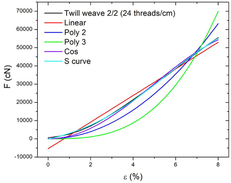
Linear, polynomial, cosine and sigmoidal fitted curves of the twill weave 2/2 fabric of 24 threads/cm density.

Table 1 lists the adjusted R-squared values of each of the models for the selected woven fabrics and the appropriate equations for the chosen fitting models. The results suggest that the fitting level depends on the type of fabric and type of chosen model. In this article, the high fitting levels (highest R²) are noticed for the plain weave (24 threads/cm) fabric for all chosen fitted models except linear (values close to 1), while the high level of fitting was provided by the cosine and sigmoidal curves models for all woven fabrics. Cosine and especially sigmoidal curves provide overall excellent accuracy, but it is worth noting that considerably simpler parabolic approximation also gives very good fit for plane weave, and even linear approximation for satin and twill weave. Maybe cubic curve would fit better for knitted fabric.

Table 1.

Curve fit equations and adj. R² values of the selected woven fabrics.

Woven fabric	Curve fit
Equation	y = A + B × x	y = A × x²	y = A × x³	y = B – B × cos(x × A)	y = A₁ + (A₂ – A₁)/(1 + 10^{((logx₀–x) × p))}
R ²
Plain weave (20 threads/cm)	0.96869	0.97200	0.81640	0.99902	0.99982
Plain weave (24 threads/cm)	0.91830	0.99842	0.93803	0.99835	0.99999
Satin 4/1(3) (24 threads/cm)	0.99334	0.88941	0.63095	0.98917	0.99967
Twill weave (24 threads/cm)	0.98097	0.94913	0.75735	0.99728	0.99956

Computational mechanical model of fabric based on parabolic tensile law

In this section, let us implement previously considered parabolic tensile approximation to a ‘structural’ situation involving fabric. As a representative situation of such type, in which there is an uneven distribution of stress, consider the tensile load on fabric specimen applied by means of a rigid crossbar with certain eccentricity, that is, non-symmetrically, Figure 5(a). Let the material be assumed as nonlinearly elastic with parabolic law, but only in the tensile range, while in the compression it has virtually zero stiffness, it is flexible and buckles easily and any compressive stress is cut to zero. The adopted stress–strain diagram is shown in Figure 5(b).

Figure 5.

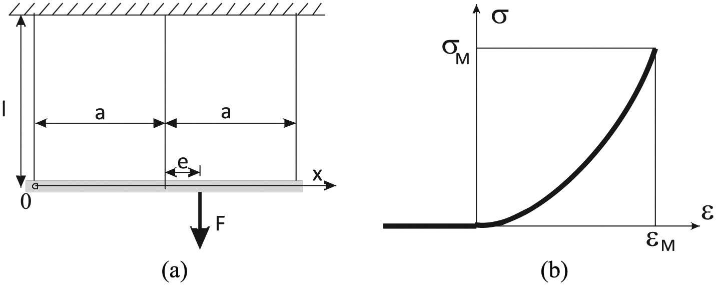
Specimen in (a) tensile loading and (b) assumed stress–strain diagram.

If stress and strain at the breaking point, as the maximum possible stress and strain in the fabric, are denoted as σ_M and ε_M, respectively (Figure 5(b)), the assumed tensile law can be written in the form

σ = k ε^{2}, k = \frac{σ_{M}}{ε_{M}^{2}}

(1)

Due to non-symmetric load, deformation of the specimen can be described by two parameters: elongation at central point v_c and angle of rotation of the crossbar ϕ (see Figure 6). First, let us try to establish the relationship between the load parameters (tensile force F and eccentricity e) and displacements v_c and ϕ. To do so, like in any stress–strain analysis, we need geometric and static conditions, on top of the material law. The displacement v of a given point of the crossbar, that is, elongation at the corresponding point of the specimen cross section, can be approximately expressed, introducing coordinate x as in Figure 5(a) or 6, in the form

v = v_{c} + φ (x - a)

(2)

Figure 6.

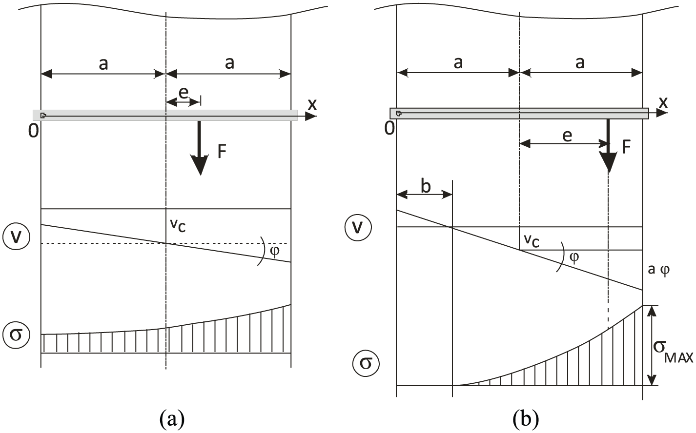
Deformed shape and stress distributions for (a) small and (b) large eccentricity.

The strain in the specimen is then, denoting by l the length of the specimen

ε = \frac{1}{l} [v_{c} + φ (x - a)]

(3)

The stress in the specimen is assumed to be uniaxial, that is, the effect of transverse constraint of the rigid crossbar and the fixed upper clamp is neglected and the stress is then

σ = \frac{k}{l^{2}} [\begin{array}{l} φ^{2} x^{2} + (2 v_{c} φ - 2 a φ^{2}) x + v_{c}^{2} \\ - 2 a v_{c} φ + φ^{2} a^{2} \end{array}]

(4)

Static conditions are in fact the equilibrium equations of the crossbar

F = \int_{ε > 0} σ d A = t \int_{ε > 0} σ d x; F (a + e) = t \int_{ε > 0} x σ d A

(5)

In equation (5), t is introduced as the thickness of the body. Let us first consider the case of small eccentricity, when v(0) > 0, that is, aϕ<v_c – the deformed shape and stress distribution are depicted in Figure 6(a).

If equation (4) is introduced to equation (5), integration in the limits from x = 0 to x = 2a gives the expressions for force F and eccentricity e in the form

F = \frac{2 a t k}{l^{2}} [v_{c}^{2} + \frac{1}{3} a^{2} φ^{2}]; e = \frac{2}{3} a \frac{v_{c} a φ}{v_{c}^{2} + \frac{1}{3} a^{2} φ^{2}}

(6)

This is valid only until aϕ=v_c or e = a/2. This corresponds to the case when the point of action of the tensile force reaches the edge of the ‘core’ of the cross section (central region in which normal force produces the stress of equal sign in all points of the cross section). For higher values of e, we talk of large eccentricity and the situation is depicted in Figure 6(b). Again, the static conditions require that the tensile force be equal to the area of the stress diagram in Figure 6(b), and that it acts in the centre of gravity of the diagram. The following equations are derived from these conditions

\begin{array}{l} b = 2 a (2 \frac{e}{a} - 1); v_{c} = (3 - 4 \frac{e}{a}) a φ; \\ F = \frac{32}{3} \frac{2 a t k}{l^{2}} {(1 - \frac{e}{a})}^{3} a^{2} φ^{2} \end{array}

(7)

Note that b represents the width of the specimen portion in which strain is negative and thus stress is equal to zero (Figure 6(b)).

Now let us consider the impact of eccentricity e to the degree of increase in maximum stress at the tensile load by a given constant value of the force F. This can be referred to as stress concentration due to load eccentricity. In the case without eccentricity, we have σ = F/2at = const., and this value of stress can be kept for later reference. In the limit case between small and large eccentricity, that is, at e = a/2, use of the formula for the area limited by parabolic arc in equilibrium of forces on the crossbar delivers the expression σ_MAX = 3 F/2at. In the case of small eccentricity, equation (6) upon elimination of aϕ lead to the following quadratic equation in $v_{c}^{2}$

v_{c}^{4} - v_{c}^{2} \frac{F l^{2}}{2 a t k} + \frac{3}{16} {(\frac{e}{a})}^{2} \frac{F^{2} l^{4}}{a^{2} t^{2} k^{2}} = 0

(8)

The solution of equation (8) is introduced, using again the relations (equation (6)), in the expression for maximum stress (equation (9))

σ_{M A X} = \frac{k}{l^{2}} {(v_{c} + a φ)}^{2}

(9)

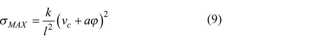
The following expression for maximum stress is then obtained

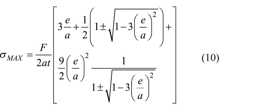
σ_{M A X} = \frac{F}{2 a t} [\begin{array}{l} 3 \frac{e}{a} + \frac{1}{2} (1 \pm \sqrt{1 - 3 {(\frac{e}{a})}^{2}}) + \\ \frac{9}{2} {(\frac{e}{a})}^{2} \frac{1}{1 \pm \sqrt{1 - 3 {(\frac{e}{a})}^{2}}} \end{array}]

(10)

Physically meaningful solution is extracted from equation (10) to comply with the mentioned σ_MAX = 3F/2at when e = a/2. The expression for maximum stress is then rearranged and reduced to

σ_{M A X} = \frac{F}{2 a t} [2 + 3 \frac{e}{a} - \sqrt{1 - 3 {(\frac{e}{a})}^{2}}]

(11)

In the case of large eccentricity (Figure 6(b)), the static condition can be written in the form

σ_{M A X} (2 a - b) \frac{t}{3} = F

(12)

The expression for maximum stress, using first of the expressions (equation (7)), takes the form

σ_{M A X} = \frac{F}{2 a t} \frac{3}{2 (1 - \frac{e}{a})}

(13)

The results (equations (11) and (13)) are shown in Table 2 and Figure 7. Maximum stress is normalised with reference to the uniform stress with zero eccentricity σ_ref = F/2at, while the eccentricity is normalised with respect to the half width of the specimen a.

Table 2.

Maximum stress in terms of force eccentricity.

e/a	0	0.1	0.2	0.3	0.4	0.5	0.6	0.7	0.8	0.85	0.9	0.95
σ_MAX/σ_ref	1	1.315	1.662	2.046	2.479	3	3.75	5	7.5	10	15	30

Figure 7.

Diagram maximum stress–eccentricity for given force F = const.

Solutions (equations (11) and (13)) are checked to provide continuity in the transition point e = a/2 not only in value, but also in slope, so in the curve in Figure 7 there is C₁ continuity in that point. Obviously, stress concentration factor defined by equation (13) tends to infinity as e approaches a.

Numerical simulation of tensile test with load eccentricity

In this section, let us try to computationally predict the outcome of the eccentric tensile test (force–displacement curve, ultimate force and elongation) based on the assumed parabolic tensile approximation, using the expressions derived in the previous section. Let the reference ultimate force be the one recorded by the usual symmetric tensile test F_M = 2atσ_M. The reduced ultimate force due to eccentricity, or as we refer to it apparent ultimate force $F_{M}^{*}$ , follows from the condition that the maximum tensile stress be equal to the ultimate stress σ_M. The apparent reduction of ultimate force follows readily from equations (11) and (13). In the case of small eccentricity e < a/2 it reads

F_{M}^{*} = \frac{F_{M}}{2 + 3 \frac{e}{a} - \sqrt{1 - 3 {(\frac{e}{a})}^{2}}}

(14)

In the case of large eccentricity e > a/2, the apparent ultimate force follows from equation (13) in the form

F_{M}^{*} = \frac{2}{3} F_{M} (1 - \frac{e}{a})

(15)

Note that the factor of ultimate force reduction would form a table similar to Table 1, in which the numbers would be reciprocal (inverse) to the factor of increase in maximum stress.

Finally, let us look for the computational prediction of the curve F – Δl of tensile test with eccentric load. The apparent elongation (displacement of the point of action of the force) can be approximately taken as

Δ l^{*} = v_{c} + e φ

(16)

In the case of small eccentricity, again the solution of equation (8) for v_c is required, along with the expression for the angle ϕ following from equation (6)

a φ = \frac{1}{v_{c}} \frac{3}{2} \frac{e}{a} \frac{F l^{2}}{2 a t k}

(17)

When the physically meaningful solution for v_c is inserted in equations (17) and (16), the apparent elongation takes the form

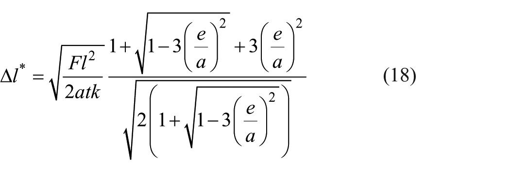
Δ l^{*} = \sqrt{\frac{F l^{2}}{2 a t k}} \frac{1 + \sqrt{1 - 3 {(\frac{e}{a})}^{2}} + 3 {(\frac{e}{a})}^{2}}{\sqrt{2 (1 + \sqrt{1 - 3 {(\frac{e}{a})}^{2}})}}

(18)

This can be squared to produce

\frac{F}{2 a t} = {(\frac{Δ l^{*}}{l})}^{2} k^{'}

(19)

This means that the apparent stress–strain curve is again parabolic, only instead of parameter k of equation (1) here we have the corrected parameter k’ due to eccentricity, which has the form

k^{'} = 2 k \frac{1 + \sqrt{1 - 3 {(\frac{e}{a})}^{2}}}{{[1 + \sqrt{1 - 3 {(\frac{e}{a})}^{2}} + 3 {(\frac{e}{a})}^{2}]}^{2}}

(20)

In the case of large eccentricity, apparent elongation (equation (16)) using equation (7) is obtained in the form

Δ l^{*} = 3 l \sqrt{\frac{3 F}{64 a t k (1 - \frac{e}{a})}}

(21)

This again produces the force–elongation relationship of the form equation (19), only now the corrected parameter k’ has the form

k^{'} = \frac{32}{27} k (1 - \frac{e}{a})

(22)

The computed relative values of correction parameter, apparent breaking force and apparent ultimate strain are given in Table 3 for four values of eccentricity.

Table 3.

Relative values of k’, $F_{M}^{*}$ and $ε_{M}^{*}$ in terms of eccentricity.

e/a	0.2	0.4	0.6	0.8
k’/k	0.915	0.7105	0.474	0.237
$F_{M}^{}$ /F_M*	0.617	0.4034	0.2667	0.1333
$ε_{M}^{}$ /ε_M*	0.811	0.7535	0.75	0.75

Computed curves relating tensile force and apparent elongation are shown in the tensile diagram of Figure 8. Note that at large eccentricities, apparent ultimate elongation remains the same regardless of the value of eccentricity, since ultimate force and parameter k are proportionally reduced, in fact, a simple calculation based on equations (15), (19) and (22) leads to ε_M^*/ε_M = 0.75 (see Table 3). This is similar to the recently reported result for simpler linear approximation in the tensile range.¹⁵

Figure 8.

Computed curves for tensile test with eccentricities.

Conclusion

Nonlinearity in tensile response of woven fabrics can be approximately described by a number of theoretical models. Trigonometric and especially sigmoidal curves provide excellent accuracy in fitting experimental tensile curves, while considerably simpler linear and second-order polynomial models offer good balance between accuracy and simplicity for some woven fabrics. The second-order parabolic approximation is applied in the example of stress–deformation analysis where the uniaxial tensile stress is distributed unevenly in the body. Tensile loading with deviation from symmetry applied by means of a rigid crossbar is considered as the representative example of such case. The analysis is performed using static and geometric conditions and the assumed approximate material law. Unlike in solid bodies, where this type of analysis is considered as combination of pure tension and pure bending, in the case of large eccentricity the carrying portion of the specimen is reduced due to the lack of compressive stress capacity, which represents the separate source of nonlinearity. The analysis can be subdivided into two separate situations: at small eccentricity tensile stress is distributed over the whole cross section, while at large eccentricity, the carrying portion is reduced. Factor of maximum stress increase theoretically tends to infinity as the relative eccentricity approaches unity. In the load–elongation simulation of tensile test with out-of-centre force, tensile diagrams indicate the reduced apparent stiffness and reduced ultimate loads due to eccentricity.

It should be noted that the present analysis does not pretend to offer general solutions, but merely a specific solution for the case when parabolic approximation is adequate (plain weave). Numbers in Table 1 suggest that trigonometric and sigmoidal approximations offer better overall fit – they could be included in the analysis in a similar way as the considered parabolic approximation, with surely more elaborate mathematical background. Solutions obtained in such a way could be considered closer to general.

One should also keep in mind the limitations due to the approximation of small rotations (equations (2) and (16)). Remember that, for example, sinϕ = ϕ is in error by under 5% at ϕ = 30^o = 0.5236 rad and by over 20% at ϕ = 60^o = 1.0476 rad. Therefore, the present analysis only holds for moderate rotations consistent with limited extensibility – the unlimited growth of stress as relative eccentricity approaches unity (Figure 7) must anyway be stopped by the onset of breaking. Possible geometric redistribution of load at large rotations is also neglected. Still, the authors do believe that within these limitations the mechanical behaviour of fabric as ‘tension only material’ as opposed to solid bodies is adequately described by the present model.

Footnotes

Declaration of conflicting interests

The author(s) declared no potential conflicts of interest with respect to the research, authorship, and/or publication of this article.

Funding

The author(s) disclosed receipt of the following financial support for the research, authorship, and/or publication of this article: This work has been fully supported by Croatian Science Foundation under the project number IP-2018-01-3170.

References

Brnada

Deformacije tkanina uvjetovane anizotropnošću [Deformation of woven fabrics caused by anisotropy, in Croatian]. PhD Thesis, Faculty of Textile Technology, University of Zagreb, Zagreb, 2017.

Barburski

Masajtis

Modeling of the change in structure of woven fabric under mechanical loading. Fibers Text East Eur 2009; 17: 39–44.

Malik

Hussain

et al . Development of models to predict tensile strength of cotton woven fabrics. J Eng Fiber Fabr 2011; 6: 46–53.

Tehrani-Dehkordi

Nosraty

Tensile behavior simulation of woven fabric with different weave pattern based on finite element method. J Text Polym 2015; 3: 34–39.

Postle

Carnaby

De Jong

The mechanics of wool structures. Chichester: Ellis Horwood, 1988.

Boisse

Gasser

Hagege

Billoet

J-L.

Analysis of the mechanical behavior of woven fibrous material using virtual tests at the unit cell level. J Mater Sci 2005; 40: 5955–5962.

Lomov

Boisse

de Luycker

et al . Full-field strain measurements in textile deformability studies. Compos Part A: Appl Sci Manuf 2008; 39: 1232–1244.

Rahnev

. Virtual energy evaluation of the fibers stress-strain state. In: Proceedings of the 14th AUTEX world textile conference, Bursa, 26–28 May 2014.

Rahnev

. Probabilistic localization of the yield point into the rheogram of the textile thread. In: Proceedings of the 15th AUTEX world textile conference, Bucharest, 10–12 June 2015.

10.

Jiang

Effect of load eccentricity on the stress-strain relationship of FRP-conﬁned concrete columns. Compos Mater 2013; 98: 228–241.

11.

Khashaba

Aldousari

Najjar

IMR

. Behavior of [0]₈ woven composites under combined bending and tension loading: part-I – experimental and analytical. J Compos Mater 2012; 46: 1345–1355.

12.

Wysmulski

Debski

Stability analysis of composite columns under eccentric load. Appl Compos Mater 2019; 26: 9743–9748.

13.

Seitl

Rios

Cifuentes

et al . Effect of the load eccentricity on fracture behaviour of cementitious materials subjected to the modified compact tension test. Solid State Phenomena 2017; 258: 518–521.

14.

Tang

Sun

Compressive behavior of sustainable steel-FRP composite bars with different slenderness ratios. Sustainability 2019; 11: 1118–1133.

15.

Šomođi