Data Inconsistency Evaluation for Cyberphysical System

Abstract

Cyberphysical systems (CPSs) have been widely applied in a variety of applications to collect data, while data is often dirty in reality. We pay attention to the way of evaluating data inconsistency which is a major concern for evaluating quality of data and its source. This paper is the first study on data inconsistency evaluation problem for CPS based on conditional functional dependencies. Given a database instance D including n tuples and a CFD set $\mathrm{\Sigma }$ including r CFDs, data inconsistency is defined as the ratio of the size of minimum culprit in D, where a culprit is a set of tuples leading to integrity errors. Firstly, we give a sufficient analysis on the complexity and inapproximability of minimum culprit problem. Then, we provide a practical algorithm that gives a 2-approximation of the data dirtiness in $O(rn\log n)$ time based on independent residual subgraph. To deal with the large dynamic data, we provide a compact structure based on B-tree for storing independent residual subgraph in order to update inconsistency efficiently. At last, we test our algorithm on both synthetic and real-life datasets; the experiment results show the scalability of our algorithm and the quality of the evaluation result.

1. Introduction

Cyberphysical Systems (CPSs) have been widely applied in a variety of applications to collect data, such as temperature, heart rate, and speed, from the physical world and make decisions based on the analysis of the data, thereby controlling and optimizing the physical objects in the real world, and they have a great influence on the way we observe and change the world [1]. CPS obtains the information of the physical world through many sensors and impacts the environment by actuators. Data sensed and sampled by sensors usually contains valuable information about the physical world, and its volume is growing. For better understanding and changing the physical environment, data collection and analysis are of the essence [2]. The knowledge extracted from the data also guides the behavior of actuators in CPS; for instance, sensors and actuators cooperate with each other to monitor some area [3] and react when a certain event is detected [4, 5]. Data gathered by sensors will not just be thrown away when they have been transmitted to the processors, but they will also be stored for further analysis. Unfortunately, not all the information gathered by different CPSs is reliable due to hardware and communication limits [6]. Many deployment experiences have shown that low data quality is the most serious problem that impacts CPS performance. Tolle et al. pointed out that faulty data can occur in various unexpected ways and less than 69% of their data could be used for meaningful interpretation [7]. Szewczyk et al. also found that about 30% of data are faulty in their deployment [8]. What makes the situation worse is that the quality of data is not easily judged. It is important to find a way to identify the quality of data gathered by CPSs to estimate the availability of data. Meanwhile, the data quality also reflects the reliability of the system. In this paper, we utilized data inconsistency to measure the data quality and we store all the data in a relational database.

Once these systems get pervasive and ubiquitously available, large amounts of data will be collected. They may include faked information. Such case highlights the quality of the data in the decision-making system and other CPSs; it is crucial for the success of the applications. Without high-quality data, no high-quality service based on the right decision could be provided, for instance, aggregation and routing services [9–15].

1.1. Motivation

In CPSs, data is collected mostly from the physical world. However, data availability would be reduced by faulty data which is not reporting the real value of the monitoring objects. The idea in this paper is that the database techniques of data inconsistency can be utilized to model and manage the data quality for CPS, in order to evaluate data source quality, CPS data quality, and so on. Based on this, we propose the new measurement and technique for its efficient computation.

In database technique, data consistency is one of the most important aspects of data quality; it is usually defined based on integrity constraints. They are semantic conditions that a database should satisfy in order to be an appropriate model of external reality. In practice, a database may not satisfy those integrity constraints, and for that reason it is said to be inconsistent or dirty. As a type of integrity constraint, conditional functional dependency (CFD) [16] has been proposed to capture inconsistency in data, which is a generalization of functional dependency (FD) [17] and has more powerful expressibility than FD. Based on CFD, many works on data quality have appeared; for example, [18–20] focus on inconsistency detection problem, while [21–26] focus on the data repairing problem. Besides inconsistency detection and data repairing, an important problem is data inconsistency evaluation which aims to quantify how dirty the data is.

Traditional evaluation methods for data source are mostly based on statistics. Compared with them, the logical method proposed in this paper is more flexible and fundamental. And the proposed method has a higher capability of expression. To the best of our knowledge, there is no existing work on providing a specific formula quantifying the data inconsistency based on CFD. We now give an example for modeling CPS data using CFDs. Consider the example below.

Example 1.

A CPS group maintains a relation of sensing data for its laboratory for several years:

$$\begin{array}{cc}& \mathrm{C}\mathrm{M}\left(\mathrm{s}\mathrm{i}\mathrm{d},\mathrm{l}\mathrm{o}\mathrm{c},\mathrm{t}\mathrm{i}\mathrm{m}\mathrm{e},\mathrm{w}\mathrm{e}\mathrm{e}\mathrm{k},\mathrm{d}\mathrm{a}\mathrm{t}\mathrm{e},\mathrm{t}\mathrm{e}\mathrm{m}\mathrm{p},\mathrm{v}\mathrm{i}\mathrm{b}\mathrm{r}\mathrm{a}\mathrm{t}\mathrm{e}\right).\end{array}$$

(1)

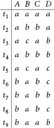
Each climate monitor tuple contains information about a record t (a unique sensor id $\mathrm{s}\mathrm{i}\mathrm{d}$ , location of sensor loc, time information about data reporting (time, week, and date), temperature, and vibrate). A sampled fragment D from all the data is shown in Table 1.

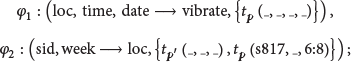
Two CFDs defined over such sampled data are shown as follows:

$$\begin{array}{cc}& {\phi }_{\mathrm{1}}:\left(\mathrm{loc},\text{\hspace{0.17em}time},\text{\hspace{0.17em}date}⟶\text{vibrate},\left\{t_p\left(\_,\_,\_,\_\right)\right\}\right),\\ {\phi }_{\mathrm{2}}:\left(\text{sid},\text{week}⟶\mathrm{loc},\left\{t_{p^{\prime }}\left(\_,\_,\_\right),t_p\left(\mathrm{s}\mathrm{817},\_,\mathrm{6}\text{:}\mathrm{8}\right)\right\}\right);\end{array}$$

(2)

intuitively, ${\phi }_{\mathrm{1}}$ restrains the notion that the vibrate status of each location is the same at the same time, while ${\phi }_{\mathrm{2}}$ specifies that the location of each sensor cannot be changed in the same week; however, for the special one “ $\mathrm{s}817$ ,” its position cannot be changed no matter the time. According to such two CFDs, D is inconsistent, since there exists violation in them as follows:

• (i)

  Tuple pair $\left(t_{\mathrm{1}},t_{\mathrm{4}}\right)$ are violations with respect to ${\phi }_{\mathrm{1}}$ , because they reported different “vibrate” status.

• (ii)

  Tuple $t_{\mathrm{4}}$ is a violation with respect to ${\phi }_{\mathrm{2}}$ , because “s817” at location “6:8” cannot be changed.

• (iii)

  Tuple pairs $\left(t_{\mathrm{1}},t_{\mathrm{3}}\right)$ and $\left(t_{\mathrm{2}},t_{\mathrm{3}}\right)$ are violations with respect to ${\phi }_{\mathrm{2}}$ , because “s816” reported different “location” at the same week.

It is easy to see that the size of minimum culprit is $\mathrm{2}$ because any culprit cannot have less than $\mathrm{2}$ tuples; for example, subset $\{t_{\mathrm{3}},t_{\mathrm{4}}\}$ is a minimum culprit. That is to say, the data we sampled is not very reliable, and, to make it clear, at least 33.3% of the data should be cleaned.

Table 1

Sampled data.

	sid	loc	Time	Week	Date	Temp.	Vibrate
$$t_{\mathit{1}}$$	s816	6:8.1	14:10	0079	11-04	48	0
$$t_{\mathit{2}}$$	s816	6:8.1	14:10	0079	11-05	24	1
$$t_{\mathit{3}}$$	s816	7:4.2	14:10	0079	11-06	22	1
$$t_{\mathit{4}}$$	s817	6:8.1	14:10	0079	11-04	24	1
$$t_{\mathit{5}}$$	s817	6:8	14:10	0080	11-09	24	0
$$t_{\mathit{6}}$$	s817	6:8	14:10	0080	11-10	22	0

Motivated by this, we consider how to efficiently compute this inconsistency measurement when the integrity constraint is conditional functional dependency in this paper. Technically, to the best of our knowledge, there is no existing work considering this aspect. There are some detection techniques [18–20, 27] but they are not able to reveal how dirty the data is directly. For confidence computation [28], our problem generalizes the confidence of a single CFD; actually, this measurement is also the confidence of a set of CFDs. For repairing techniques, our problem can be seen as a special case of [29], because the complementary minimum culprit can be seen as C-repair (cardinality repair) of an inconsistent database; however, it is much more expensive using the techniques proposed by [29] directly, especially for dynamic data, and the algorithm given in this paper is more efficient and seems optimal. Briefly, there are three challenges. $(1)$ The first challenge is how to evaluate the inconsistency efficiently. It is proved that the inconsistency evaluation problem we study is NP-complete even if there are only two CFDs in rule set and there are only three attributes in relation schema. Therefore, we should provide an efficient approximation algorithm for evaluating the data inconsistency. $(2)$ Because most existing repair algorithms that could perform repair encounter a huge searching space when data is large and they have to take an expensive cost on performance, the approximation algorithm is also expected to be more efficient than the C-repair algorithms and to be able to guarantee the approximation ratio and evaluate large data more than data in memory. $(3)$ For the dynamic data, an external memory data structure is necessary to make the approximation algorithm able to deal with the update of tuples efficiently rather than recomputing the inconsistency from scratch.

1.2. Contributions

This paper first studies how to compute the data inconsistency for CPS data efficiently with respect to CFDs; the main contributions in this paper are as follows:

• (a)

We formally define the inconsistency evaluation problem. The inconsistency of a given database instance D is defined based on minimum culprit, the minimum subset of D, whose complementary value in D is consistent with respect to all the given CFDs, and we use the proportion of minimum culprit to quantize the inconsistency of a database. It is proved that it is monotonic and insensitive to a small change on the database. And we prove that the minimum culprit problem is still NP-complete even if $(1)$   Σ has only two variable CFDs; $(2)$ the relation has only $\mathrm{3}$ attributes; and $(3)$ the number of violations caused by each tuple is not more than $\mathrm{6}$ .

(b)

Based on the conflict graph model, we transform the inconsistency evaluation problem into the minimum vertex cover problem based on conflict graph model. Based on finding the maximal matching of independent residual subgraph, we give a $\mathrm{2}$ -approximation algorithm with $O\left(rn\log n\right)$ time complexity where r is the number of given CFDs and always a small constant. To deal with large dynamic data, we design a compact structure for indexing all tuples and give the method for its maintenance. Some useful properties of independent residual subgraph prevent storing edges in the compact structure so that the storage cost of the graph is $O\left(rn\right)$ and the update cost is only $O\left(r\log n\right)$ .

(c)

Using TPCH for large-scale data and IMDB and DBLP for real-life data, we conduct experiments on PC. We find that the adjusted counterpart outperforms the evaluation algorithm if several CFDs are of small confidence while the others are not. In addition, our algorithms scale well with both the size of the data and the number of CFDs.

2. Background

An l-ary relation schema can be represented by $R(A_{\mathrm{1}},A_{\mathrm{2}},\dots ,A_l)$ , where R is the relation name and all $A_j$ 's ( $\mathrm{1}\le j\le l$ ) are the attributes of R. Let $\mathrm{a}\mathrm{t}\mathrm{t}\mathrm{r}(R)$ be $\{A_{\mathrm{1}},\dots ,A_l\}$ , and let $\mathrm{d}\mathrm{o}\mathrm{m}(A_j)$ be the domain of attribute $A_j$ . An instance D of relation R is a set of l-ary tuples, denoted by $D=\{t_{\mathrm{1}},t_{\mathrm{2}},\dots ,t_n\}$ , where each tuple $t_i\mathrm{\hspace{0.17em}\hspace{0.17em}}(\mathrm{1}\le i\le n)$ belongs to the set $\mathrm{d}\mathrm{o}\mathrm{m}(A_{\mathrm{1}})\times \mathrm{d}\mathrm{o}\mathrm{m}(A_{\mathrm{2}})\times \cdots \times \mathrm{d}\mathrm{o}\mathrm{m}(A_l)$ . Let $t_i\left[A_j\right]$ be the value of $t_i$ on attribute $A_j$ .

Conditional functional dependency, CFD for short, is a class of integrity constraints capturing the consistency of data, whose formal definition can be found in [24]. Next, the syntax and semantic definitions of CFD will be reviewed briefly.

• (i)

Syntax. A CFD rule φ defined over relation R is a pair $(X\to Y,T_p)$ , where X and Y are two distinctive attribute lists satisfying $X\cup Y\subseteq \mathrm{a}\mathrm{t}\mathrm{t}\mathrm{r}\left(R\right)$ , $X\to Y$ is a standard FD, and $T_p$ is a pattern tableau over attributes $X\cup Y$ . For each tuple $t_p\in T_p$ and each attribute $A\in X\cup Y$ , the value $t_p[A]$ can be either a constant “a” in $\mathrm{d}\mathrm{o}\mathrm{m}(A)$ or a wild card “_”. For a rule φ, we use $\mathrm{L}\mathrm{H}\mathrm{S}(\phi )$ to denote X and $\mathrm{R}\mathrm{H}\mathrm{S}(\phi )$ to denote Y.

(ii)

Semantic. Given a tuple t and a pattern tuple $t_p$ , t is said to match $t_p$ , denoted by $t\asymp t_p$ , if either $t[A]=t_p[A]$ or $t_p[A]$ = “_” is satisfied for each attribute A. Two tuples $t_{\mathrm{1}}$ and $t_{\mathrm{2}}$ satisfy φ, denoted by $\left(t_{\mathrm{1}},t_{\mathrm{2}}\right)\models \phi$ , if when $t_{\mathrm{1}}[X]=t_{\mathrm{2}}[X]\asymp t_p[X]$ , there must be $t_{\mathrm{1}}[Y]=t_{\mathrm{2}}[Y]\asymp t_p[Y]$ ; if $t_{\mathrm{1}}[X]=t_{\mathrm{2}}[X]\asymp t_p[X]$ but $t_{\mathrm{1}}[Y]\ne t_{\mathrm{2}}[Y]$ , then tuple pair $\left(t_{\mathrm{1}},t_{\mathrm{2}}\right)$ is a violation. Particularly, a single tuple $t\models \phi$ , if when $t[X]\asymp t_p[X]$ , we must have $t[Y]\asymp t_p[Y]$ . Given a relational instance D and a CFD rule φ, D is said to satisfy φ (i.e., $D\models \phi$ ) iff, (a) for each tuple $t\in D$ , $t\models \phi$ and, (b) for any two tuples $t_{\mathrm{1}}$ and $t_{\mathrm{2}}$ in D, $\left(t_{\mathrm{1}},t_{\mathrm{2}}\right)\models \phi$ . Given a CFD set Σ, D is consistent with respect to Σ, if it satisfies all rules in set Σ; otherwise, it is inconsistent or dirty, denoted by $D⊭\Sigma$ . For example, in Table 1, tuple pair $\left(t_{\mathrm{1}},t_{\mathrm{2}}\right)$ is a violation with respect to ${\phi }_{\mathrm{1}}$ shown in Example 1 (i.e., $\left(t_{\mathrm{1}},t_{\mathrm{2}}\right)⊭{\phi }_{\mathrm{1}}$ ) due to the fact that “ $t_{\mathrm{1}}[\mathrm{l}\mathrm{o}\mathrm{c},\mathrm{t}\mathrm{i}\mathrm{m}\mathrm{e},\mathrm{d}\mathrm{a}\mathrm{t}\mathrm{e}]=t_{\mathrm{4}}[\mathrm{l}\mathrm{o}\mathrm{c},\mathrm{t}\mathrm{i}\mathrm{m}\mathrm{e},\mathrm{d}\mathrm{a}\mathrm{t}\mathrm{e}]\asymp t_p[\mathrm{l}\mathrm{o}\mathrm{c},\mathrm{t}\mathrm{i}\mathrm{m}\mathrm{e},\mathrm{d}\mathrm{a}\mathrm{t}\mathrm{e}]$ ”, but “ $t_{\mathrm{1}}[\mathrm{v}\mathrm{i}\mathrm{b}\mathrm{r}\mathrm{a}\mathrm{t}\mathrm{e}]=$ ‘0’ $\ne t_{\mathrm{4}}[\mathrm{v}\mathrm{i}\mathrm{b}\mathrm{r}\mathrm{a}\mathrm{t}\mathrm{e}]=$ ‘1’”; therefore, D is inconsistent or dirty because of the existence of violation.

A CFD is said to be simple if there is only one row in its pattern tableau such as both CFDs shown in Example 1. Additionally, two special fragments of simple CFD can be defined as follows:

• (i)

A simple CFD $\phi =(X\to Y,T_p)$ is said to be a variable CFD, if, for each $A\in Y$ , $t_p[A]\ne$ “_”; for example, ${\phi }_{\mathrm{1}}$ is a variable CFD.

(ii)

A simple CFD $\phi =(X\to Y,T_p)$ is said to be a constant CFD, if, for each $A\in Y$ , $t_p[A]=$ “_”; for example, the second pattern of ${\phi }_{\mathrm{2}}$ can be changed into a constant CFD.

Intuitively, a constant CFD can capture inconsistencies on single tuple, while a variable CFD can capture inconsistencies between two tuples.

In fact, given any CFD, it can be rewritten by some simple CFDs naïvely by splitting its tableau horizontally, while a simple CFD can be rewritten by at most a constant one and a variable one. Therefore, without loss of generality, only simple CFDs are used in this paper.

3. Problem Definition

This section first formally defines the data inconsistency evaluation problem and then proves that it is NP-complete.

Given a CFD set Σ and a database instance D such that $D⊭\Sigma$ , intuitively, the dirty part $D^{\prime }$ is a subset of D such that the deletion of $D^{\prime }$ will make the data clean. We can formalize this idea as follows.

Definition 2 (culprit).

Given a database instance D and a set of CFD rules Σ, culprit $C\left(D\right)$ is a subset of D satisfying $D-C\left(D\right)\models \Sigma$ .

Obviously, for fixed Σ and D, there may be many culprits. In this paper, to measure the data dirtiness, we only care about the minimum culprit. $C_{\mathrm{m}\mathrm{i}\mathrm{n}}\left(D\right)$ is the minimum culprit if, for any culprit $C\left(D\right)$ , $\left|C_{\mathrm{m}\mathrm{i}\mathrm{n}}\left(D\right)\right|\le \left|C\left(D\right)\right|$ .

Definition 3 (data dirtiness evaluation problem).

Given a database instance D and a set of CFD rules Σ, we want to compute the dirtiness of a database instance D, which is $\mathrm{d}\mathrm{i}\mathrm{r}\mathrm{t}(D,\Sigma )=\left|C_{\mathrm{m}\mathrm{i}\mathrm{n}}\left(D\right)\right|/\left|D\right|$ .

Property 1 (minimality).

Given any instance D and any CFD set Σ, $\mathrm{d}\mathrm{i}\mathrm{r}\mathrm{t}\left(D,\Sigma \right)$ is the portion of tuples that need to be edited at least in any exact repair algorithm.

Measurement $\mathrm{d}\mathrm{i}\mathrm{r}\mathrm{t}\left(D,\Sigma \right)$ is also monotonic and insensitive to a small change Δ (i.e., set of tuples) on instance D as the following proposition states.

Property 2 (monotonic and insensitive).

Given an instance D, a set of tuples Δ, and CFD set Σ, we have $\mathrm{0}\le \left|C_{\mathrm{m}\mathrm{i}\mathrm{n}}\left(D\cup \Delta \right)\right|-\left|C_{\mathrm{m}\mathrm{i}\mathrm{n}}\left(D\right)\right|\le \left|\Delta \right|$ .

This implies $\mathrm{0}\le |\mathrm{d}\mathrm{i}\mathrm{r}\mathrm{t}(D\cup \Delta ,\Sigma )-\mathrm{d}\mathrm{i}\mathrm{r}\mathrm{t}(D,\Sigma )|\le \left|\Delta \right|/(|D|+|\Delta |)$ .

Remark 4.

That is to say, the inconsistency of data measured by Definition 2 changes gently with small update. Usually, this trend of variation agrees with the reality; this is really because “(1) most of the data is often correct, especially for large data, and (2) a small update has a tiny impact on the dirtiness of the entire dataset.”

Similar to [30], we next have the following theorem on the complexity of minimum culprit problem with more restricted condition on the input. Here, the decision version of minimum culprit problem, k-culprit problem for short, is that, given a database instance D and a CFD set Σ, it is to decide whether there is a culprit C of D with respect to Σ and the size $\left|C\right|\le k$ .

Theorem 5.

Given an instance D of relation R and CFD set Σ, k-culprit problem is NP-complete, even if (1) there are only 2 variable CFDs in Σ, (2) R is a 3-ary relation, and (3) for each tuple $t\in D$ there are at most 6 violations including t.

Proof.

 

NP. There is an NP algorithm as follows: $(1)$ guess a subset C of D with size of k; $(2)$ check whether $D-C\models \Sigma$ , that is, to check whether each tuple pair in $D-C$ satisfies all CFDs of Σ; $(3)$ output “ $yes$ ” when $D-C\models \Sigma$ and “ $no$ ” otherwise. For each instantiation, the checking step can be done in polynomial time. Thus, the problem is in NP.

NP-Hardness. The lower bound is established by a reduction from $\mathrm{3}$ -SAT problem to k-culprit problem. An instance of $\mathrm{3}$ -SAT problem includes a set U of n variables $x_{\mathrm{0}},\dots ,x_{n-\mathrm{1}}$ and a collection S of m clauses $s_{\mathrm{0}},\dots ,s_{m-\mathrm{1}}$ , while, in each clause $s_j={\alpha }_{j\mathrm{1}}+{\alpha }_{j\mathrm{2}}+{\alpha }_{j\mathrm{3}}$ , each ${\alpha }_{jq}\mathrm{\hspace{0.17em}\hspace{0.17em}}(\mathrm{1}\le q\le \mathrm{3})$ is the qth literal of $s_j$ . Given an instance of $\mathrm{3}$ -SAT problem, it is to decide whether there is a satisfying truth assignment for S. The $\mathrm{3}$ -SAT problem is NP-complete, and it remains NP-complete even if, for each $x_i\in U$ , there are at most $\mathrm{5}$ clauses in S that contain either $x_i$ or ${\overline{x}}_i$ .

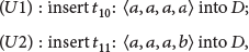
A polynomial reduction from $\mathrm{3}$ -SAT to k-culprit problem can be constructed as follows. $(1)$ Given an instance of $\mathrm{3}$ -SAT, we introduce a 3-ary relation $R\left(A,B,C\right)$ and a variable CFD set Σ including ${\phi }_{\mathrm{1}}:\left(A\to B,\left\{t_p\left(\_,\_\right)\right\}\right)$ and ${\phi }_{\mathrm{2}}:\left(C\to B,\left\{t_p\left(\_,\_\right)\right\}\right)$ . $(2)$ Build an instance D over R. For each variable $x_i$ , insert two tuples $t_{\mathrm{2}i}\left(x_i,x_i,x_i\right)$ and $t_{\mathrm{2}i+\mathrm{1}}\left(x_i,{\overline{x}}_i,x_i\right)$ into D. For each literal ${\alpha }_{jq}$ in clause $S_j$ , if it is a positive literal of variable $x_i$ , add tuple $t_{\mathrm{2}n+\mathrm{3}j+k}\left(s_j,x_i,x_i\right)$ to D; if it is a positive literal of variable $x_i$ , add tuple $t_{\mathrm{2}n+\mathrm{3}j+k}\left(s_j,{\overline{x}}_i,x_i\right)$ to D. (3) At last, let $k=n+\mathrm{2}m$ . Note that $(1)$ the instance D can be constructed in $O\left(n+m\right)$ ; $(2)$ there are $\mathrm{3}$ attributes in R and two variable CFDs in Σ; $(3)$ for each tuple t in T the number of violations caused by t is at most $\mathrm{6}$ , if each variable exhibits at most $\mathrm{5}$ clauses.

Suppose that the $\mathrm{3}$ -SAT instance is satisfiable; that is, there is a satisfying truth assignment $\rho :U\to {\left\{\mathrm{0,1}\right\}}^n$ for S; then, there is a culprit C of D such that its size is at most $n+\mathrm{2}m$ . Concretely, it can be computed as follows, for each variable $x_i$ ; $(1)$ if $\rho \left(x_i\right)=\mathrm{1}$ , delete tuple $t_{\mathrm{2}i}$ from D. Then, for each clause $s_j$ , if ${\alpha }_{jq}$ is a positive literal of $x_i$ and $t_{\mathrm{2}n+\mathrm{3}j+\mathrm{1}},t_{\mathrm{2}n+\mathrm{3}j+\mathrm{2}},t_{\mathrm{2}n+\mathrm{3}j+\mathrm{3}}\in D$ , delete $t_{\mathrm{2}n+\mathrm{3}j+q}$ from D; $(2)$ if $\rho \left(x_i\right)=\mathrm{0}$ , delete tuple $t_{\mathrm{2}i+\mathrm{1}}$ from D. Then, for each clause $s_j$ , if ${\alpha }_{jq}$ is a negative literal of $x_i$ and $t_{\mathrm{2}n+\mathrm{3}j+\mathrm{1}}$ , $t_{\mathrm{2}n+\mathrm{3}j+\mathrm{2}}$ , and $t_{\mathrm{2}n+\mathrm{3}j+\mathrm{3}}\in D$ , delete $t_{\mathrm{2}n+\mathrm{3}j+q}$ from D. We have that, for each i, either $t_{\mathrm{2}i}$ or $t_{\mathrm{2}i+\mathrm{1}}$ is deleted from D, and, for each j, either of $\left\{t_{\mathrm{2}n+\mathrm{3}j+\mathrm{1}},t_{\mathrm{2}n+\mathrm{3}j+\mathrm{2}},t_{\mathrm{2}n+\mathrm{3}j+\mathrm{3}}\right\}$ is deleted from D for each j. This is because, in each clause, there is at least one literal that is made $true$ by assignment ρ . Therefore, there is a set C of the rest of the tuples such that $D-C\models \Sigma$ and $\left|C\right|\le n+\mathrm{2}m=k$ .

To see the converse, let C be the culprit such that $\left|C\right|\le k=n+\mathrm{2}m$ . CFD ${\phi }_{\mathrm{1}}$ restricts the notion that either $t_{\mathrm{2}i}$ or $t_{\mathrm{2}i+\mathrm{1}}$ should be deleted from D, for each $\mathrm{0}\le i\le n-\mathrm{1}$ , and at least two tuples of $\left\{t_{\mathrm{2}n+\mathrm{3}j+\mathrm{1}},t_{\mathrm{2}n+\mathrm{3}j+\mathrm{1}},t_{\mathrm{2}n+\mathrm{3}j+\mathrm{1}}\right\}$ should be deleted from D. That is, the size of C is at least $n+\mathrm{2}m$ . Therefore $\left|C\right|$ is exactly $n+\mathrm{2}m$ . Moreover, CFD ${\phi }_{\mathrm{2}}$ restricts the notion that there is only one literal of each variable in $D-C$ . Then, there is a satisfying truth assignment ρ for S such that, for each $\mathrm{0}\le i\le n-\mathrm{1}$ ,

$$\begin{array}{cc}& \rho \left(x_i\right)=\left\{\begin{array}{cc}\mathrm{0}\hfill & \mathrm{i}\mathrm{f}\hspace{0.17em}\hspace{0.17em}{t}_{\mathrm{2}i}\in C,\hfill \\ \mathrm{1}\hfill & \mathrm{i}\mathrm{f}\hspace{0.17em}\hspace{0.17em}{t}_{\mathrm{2}i+\mathrm{1}}\in C.\hfill \end{array}\right.\end{array}$$

(3)

4. Evaluation Algorithm

For any database instance D, let $D_s$ be the subset of D where each tuple violates at least one constant CFD in Σ; then, we have

$$\begin{array}{cc}& C_{\mathrm{m}\mathrm{i}\mathrm{n}}\left(D\right)=\left|D_s\right|+\left|C_{\mathrm{m}\mathrm{i}\mathrm{n}}\left(D-D_s\right)\right|;\end{array}$$

(4)

this is because any culprit C of D satisfying $C-D_s$ must be larger than $C_{\mathrm{m}\mathrm{i}\mathrm{n}}\left(D-D_s\right)$ . Therefore, data dirtiness can be computed as

$$\begin{array}{cc}& \mathrm{d}\mathrm{i}\mathrm{r}\mathrm{t}\left(D,\Sigma \right)=\frac{\left|D_s\right|+\left|C_{\mathrm{m}\mathrm{i}\mathrm{n}}\left(D-D_s\right)\right|}{\left|D\right|},\end{array}$$

(5)

where $D_s$ can be detected by scanning the database once. Without loss of generality, we do not let Σ contain constant CFD from now on.

Definition 6 (conflict graph [31]).

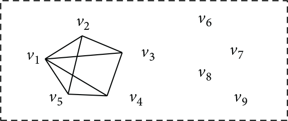
Given an instance D and a CFD set Σ with r CFDs, the conflict graph $G\left(D,\Sigma \right)$ is an undirected graph $〈V,E〉$ , where V is the vertex set and E is the edge set. In conflict graph $G\left(D,\Sigma \right)$ , each vertex $v_i\in V$ refers to the tuple $t_i\in D$ and edge $v_i{v}_j\in E$ , if $\exists \phi \in \Sigma$ , $\left(t_i,t_j\right)⊭\phi$ .

Example 7.

One has instance D with tuples $t_{\mathrm{1}}~t_{\mathrm{9}}$ as in (6) and $\Sigma =\left\{{\phi }_{\mathrm{1}}:\left(A\to B,\left\{t_p\left(\_,\_\right)\right\}\right),{\phi }_{\mathrm{2}}:\left(C\to D,\left\{t_p\left(\_,\_\right)\right\}\right)\right\}$ .

Instance D is shown as follows:

$$\begin{array}{cc}& \begin{array}{c}\begin{array}{c}\begin{array}{ccccc}& A& B& C& D\\ t_1& a& a& a& a\\ t_2& a& b& b& a\\ t_3& a& c& a& b\\ t_4& a& b& b& b\\ t_5& a& c& a& c\\ t_6& b& a& b& c\\ t_7& b& a& b& b\\ t_8& b& a& b& c\\ t_9& b& a& a& b\end{array}\end{array}\end{array}\end{array}$$

(6)

Conflict graphs $G\left(D,\Sigma \right)$ , $G\left(D,\left\{{\phi }_{\mathrm{1}}\right\}\right)$ , and $G\left(D,\left\{{\phi }_{\mathrm{2}}\right\}\right)$ are shown in Figures 1, 2, and 3. We see that $v_{\mathrm{1}}$ is adjacent to $v_{\mathrm{2}}$ because $t_{\mathrm{1}}$ conflicts with $t_{\mathrm{2}}$ with respect to ${\phi }_{\mathrm{1}}$ ; they have the same value on A but different values on B. Obviously, both $G\left(D,\left\{{\phi }_{\mathrm{1}}\right\}\right)$ and $G\left(D,\left\{{\phi }_{\mathrm{2}}\right\}\right)$ are the subgraphs of $G\left(D,\Sigma \right)$ .

Figure 1

Conflict graph $G(D,\Sigma )$ .

Figure 2

$G(D$ , $\left\{{\phi }_{\mathrm{1}}\right\})$ .

Figure 3

$G(D$ , $\left\{{\phi }_{\mathrm{2}}\right\})$ .

There is a naïve $\mathrm{2}$ -approximate algorithm (Algorithm 1). The minimum culprit can be transformed as the minimum vertex cover on the conflict graph which can be built by the input database and CFDs, and it is easy to see that the size of minimum vertex cover of the conflict graph $G\left(D,\Sigma \right)$ equals the size of minimum culprit of D. Therefore, a naïve $\mathrm{2}$ -approximation algorithm (Algorithm 1) will be obtained immediately.

Algorithm 1: Linear algorithm.

Input: Database instance D = $\left\{t_{\mathit{1}},\dots ,t_n\right\}$ , CFD set $\mathrm{\Sigma }=\left\{{\phi }_{\mathit{1}},\dots ,{\phi }_r\right\}$ .

Output: $\mathrm{d}\mathrm{i}\mathrm{r}\mathrm{t}(D,\mathrm{\Sigma })$ which is the dirtiness of database D w.r.t. $\mathrm{\Sigma }$ .

(1) $G\left(V,E\right)\leftarrow \left(\mathrm{⌀},\mathrm{⌀}\right)$ , $M\leftarrow \mathrm{⌀}$ ;

(2) for all  tuple pair $\left(t_i,t_j\right)$ in D  do

(3)  for all   ${\phi }_k\in \mathrm{\Sigma }$ such that $\mathrm{1}\le k\le r$   do

(4)   if   $(t_i,t_j)⊭{\phi }_k$   then

(5)    add vertices $v_i$ and $v_j$ into V;

(6)    add edge $v_i{v}_j$ into E;

(7)    GOTO line (2);

(8) $M\leftarrow MaximalMatching(G(V,E))$ ;

(9) return   $\mathrm{2}\left|M\right|/\left|D\right|$ ;

Algorithm 1 works like this: lines (1)–(6): build a conflict graph G for the given database instance D and the CFD set Σ; line (7): compute the minimum vertex cover approximately. One can call the classic approximation algorithm [32] to find maximal matching $M\left(G\left(D,\Sigma \right)\right)$ greedily, where a matching in G is a set of pairwise nonadjacent edges and the matching is maximal if it is not a proper subset of any other matching in G. For any maximal matching M, the amount of vertexes in M (i.e., $\mathrm{2}\left|M\right|$ ) is at most twice as much as the size of minimum vertex cover, a $\mathrm{2}$ -approximation of $\left|C_{\mathrm{m}\mathrm{i}\mathrm{n}}\left(D\right)\right|$ .

5. Reduce Quadratic for Large Dynamic Data

We propose another $\mathrm{2}$ -approximation dirtiness evaluation algorithm DDEva to overcome the shortcomings stated above. Then, an index based on B-tree is designed to enable $O\left(rn\log n\right)$ time and $O\left(rn\right)$ space implementation of DDEva over large data, where r is the number of CFDs given in a general form rather than a simple CFD. It prevents the potential quadratic storage of edges. At last, an $O\left(r\log n\right)$ update method based on the efficient update of maximal matching and conflict graph is proposed to deal with dynamic data. Generally, the number of general CFDs, r, is a small constant, so that the algorithm we proposed works efficiently as shown in the experiments. We still use simple CFD in order to simplify the description below, but note that our algorithm can process the general CFDs natively.

5.1. Some Notations and Observations

For clarity, we first declare the following notations formally. (A) Given a CFD set Σ, it has r variable CFDs, and the jth CFD is ${\phi }_j$ . The conflict graph $G\left(D,\left\{{\phi }_j\right\}\right)$ is denoted by $G_j$ for short. Recall Definition 6; obviously, $G_j$ is a subgraph of $G\left(D,\Sigma \right)$ . (B) For any matching M, let $V_M$ be the set of all vertices in M. The size of M is denoted by $\left|M\right|$ which is the number of edges in it; obviously, $\left|V_M\right|=\mathrm{2}\times \left|M\right|$ . For any graph G, let $M\left(G\right)$ be the maximal matching of G; (C) given a graph $G\left(V,E\right)$ and a matching M, let $G-M$ be a graph $G^{\prime }\left(V^{\prime },E^{\prime }\right)$ , where $V^{\prime }=V\setminus V_M$ and $E^{\prime }$ is obtained by removing all edges covered by $V_M$ from E; (D) let $K_{{\omega }_{\mathrm{1}},\dots ,{\omega }_l}$ represent a complete multipartite graph with l vertex equiv-classes, such that any pair of vertices in the same equiv-class ω are nonadjacent while any pair of vertices in different equiv-classes are adjacent. For each equiv-class ${\omega }_i$ , let $\left|{\omega }_i\right|$ be the number of vertices in it.

Given a CFD set Σ of r variable CFDs, let $G_j$ be the conflict graph $G\left(D,\left\{{\phi }_j\right\}\right)$ . Interestingly, we have the following useful observation of conflict graph with respect to one CFD.

Observation 1.

Each conflict graph $G_j$ is a forest of multipartite graph; that is, it is composed of several nonoverlapping connected components, and each component is a complete multipartite graph.

It is easy to find maximal matching for each complete multipartite connected component in each $G_j$ . However, the sum of each $G_j$ 's maximal matching sizes is not a $\mathrm{2}$ -approximation of minimum vertex cover due to the overlaps among those matching scenarios. In order to remove these overlaps, we next define a series of independent residual subgraphs $〈{\Delta }_{\mathrm{1}},\dots ,{\Delta }_r〉$ for $G\left(D,\Sigma \right)$ , in which each ${\Delta }_j$ is a counterpart of the conflict graph $G_j$ .

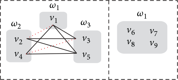
Definition 8 (independent residual subgraph).

Given a database instance D and CFD set $\Sigma =\left\{{\phi }_j\mid \mathrm{1}\le j\le r\right\}$ , the independent residual subgraph is a subgraph of $G\left(D,\Sigma \right)$ , ir-subgraph for short, such that

$$\begin{array}{cc}& {\Delta }_j=\left\{\begin{array}{cc}{G}_{\mathrm{1}}\hfill & \text{if\hspace{0.17em}\hspace{0.17em}}j=\mathrm{1},\hfill \\ G_j-M_{\mathrm{1},j-\mathrm{1}}\hfill & \text{if\hspace{0.17em}\hspace{0.17em}}\mathrm{1}<j\le r,\hfill \end{array}\right.\end{array}$$

(7)

where $M_{\mathrm{1},j-\mathrm{1}}={\bigcup }_{i=\mathrm{1}}^{j-\mathrm{1}}‍M\left({\Delta }_i\right)$ .

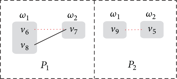
Following Example 7, Figure 4 shows ${\Delta }_{\mathrm{1}}=G_{\mathrm{1}}$ with the dash line, and Figure 5 shows ${\Delta }_{\mathrm{2}}=G_{\mathrm{2}}-M\left({\Delta }_{\mathrm{1}}\right)$ ; ${\Delta }_{\mathrm{2}}$ is obtained by removing all the vertexes $v_{\mathrm{1}}$ , $v_{\mathrm{2}}$ , $v_{\mathrm{3}}$ , and $v_{\mathrm{4}}$ and their adjacent edges from G since such four vertexes are all in the maximal matching of ${\Delta }_{\mathrm{1}}$ represented by dash edges.

Figure 4

${\Delta }_{\mathrm{1}}$ and $M\left({\Delta }_{\mathrm{1}}\right)$ .

Figure 5

${\Delta }_{\mathrm{2}}$ and $M\left({\Delta }_{\mathrm{2}}\right)$ .

Observation 2.

Each ir-subgraph ${\Delta }_j$ is also a forest of complete multipartite graph.

This observation is correct because ${\Delta }_j$ is still a complete multipartite graph when any vertex v and its adjacent edges are removed from $G_j$ . For example, in Figure 5, ${\Delta }_{\mathrm{2}}$ is still a forest of complete multipartite graph.

Interestingly, we find that the union of maximal matchings $M\left({\Delta }_{\mathrm{1}}\right)$ (dash edges in Figure 4) and $M\left({\Delta }_{\mathrm{2}}\right)$ (dash edges in Figure 5) is exactly a maximal matching of $G\left(D,\Sigma \right)$ (dash edges in Figure 6). This inspires a proposition for computing the maximal matching of conflict graph $G\left(D,\Sigma \right)$ as follows.

Figure 6

Maximal matching $M(G)$ .

Proposition 9.

$M_{\mathrm{1},r}$ is a maximal matching of $G\left(D,\Sigma \right)$ , and $\left|M_{\mathrm{1},r}\right|={\sum }_{j=\mathrm{1}}^r\left|M\left({\Delta }_j\right)\right|$ .

5.2. Algorithm for Dirtiness Evaluation

In contrast to the naïve algorithm, we propose Algorithm 2 to compute the data dirtiness in an $O\left(rn\log n\right)$ time rather than the quadratic cost while r is a small constant generally. It works as follows: r ir-subgraphs are built first instead of the conflict graph $G\left(D,\Sigma \right)$ ; compute maximal matching of each ir-subgraph independently to get the value $\left|V_{M_{\mathrm{1},r}}\right|$ which is a $\mathrm{2}$ -approximation of the size of minimum vertex cover. Proposition 9 guarantees the correctness of this algorithm.

Algorithm 2: $DDEva(D,\mathrm{\Sigma })$ .

Input: Database instance D, CFD set $\mathrm{\Sigma }=\left\{{\phi }_j\mid \mathit{1}\le j\le r\right\}$ .

Output: $\mathrm{d}\mathrm{i}\mathrm{r}\mathrm{t}(D,\mathrm{\Sigma })$ which is the dirtiness of database D with respect to $\mathrm{\Sigma }$ .

(1)  $M\leftarrow \mathrm{⌀}$ ;

(2) for all  j such that $\mathrm{1}\le j\le r$   do

(3)  build $G_j$ for D with respect to ${\phi }_j$ ;

(4)   ${\mathrm{\Delta }}_j\leftarrow G_j$ ;

(5)  for all   $v_i\in {\mathrm{\Delta }}_j$   do

(6)   if   $v_i\in M$   then

(7)    remove $v_i$ and its adjacent edges from ${\mathrm{\Delta }}_j$ ;

(8)   $M({\mathrm{\Delta }}_j)\leftarrow GreedyMaximalMatching({\mathrm{\Delta }}_j)$ ;

(9)   $M\leftarrow M\cup M({\mathrm{\Delta }}_j)$ ;

(10) return   $|V_M|/|D|$ ;

Briefly, there are two key points to reduce the quadratic cost, respectively; each ir-subgraph ${\Delta }_j$ can be built within $O\left(n\log n\right)$ , and the maximal matching of each ir-subgraph can be specified quickly without scanning any edge of it.

5.2.1. Building ir-Subgraphs

Let the jth CFD be ${\phi }_j:\left(X\to Y,T_p\right)$ ; to get ${\Delta }_j$ , we will build the conflict graph $G_j$ first and then remove all vertices of $V_{M_{\mathrm{1},j-\mathrm{1}}}$ and their adjacent edges. Recall Observation 1; each connected component of $G_j$ is a complete multipartite graph which can be built by partitioning without pairwise comparison. Concretely, we can partition all tuples of D according to the attribute values on X and Y; each connected component refers to the tuples with the same attribute value on X, and each equiv-class in the component refers to the tuples with the same attribute value on Y. Because we do not need to store edges in complete multipartite graph, only vertices in $V_{M_{\mathrm{1},j-\mathrm{1}}}$ need to be removed from $G_j$ . As the size of $V_{M_{\mathrm{1},j-\mathrm{1}}}$ is always no more than n, it will take at most $O\left(\log n\right)$ time cost to check whether a vertex $v\in V_{M_{\mathrm{1},j-\mathrm{1}}}$ based on a lookup data structure. Therefore, an ir-subgraph can be built within an $O\left(rn\log n\right)$ time.

5.2.2. Finding Maximal Matching Greedily

Due to Observation 2, each connected component of ir-subgraph is also a complete multipartite graph. We can quickly specify an arbitrary maximal matching of each connected component without scanning any edge so that the time cost for computing the maximal matching only depends on the number of vertices rather than edges.

Algorithm 3 is proposed to find a maximal matching quickly. Concretely, the maximal matching of each ir-subgraph can be obtained by the union of the maximal matchings of each component. For each component $P_i$ containing l equiv-classes, namely, ${\omega }_{\mathrm{1}},\dots ,{\omega }_l$ , we group the l equiv-classes into two groups $〈L,R〉$ . During the scan on $P_i$ , each equiv-class is added to the group with smaller cardinality greedily where cardinality of a group S is $\left|S\right|={\sum }_{i=\mathrm{1}}^s\left|{\omega }_i\right|$ , if $S=\left\{{\omega }_{\mathrm{1}},\dots ,{\omega }_s\right\}$ . Then, for a grouping $〈L,R〉$ , we build the maximal matching $M〈L,R〉$ like this; for each vertex in group L, match it with a vertex of R orderly. The time cost of Algorithm 3 does not depend on the number of edges but only depends on the number of vertexes.

Algorithm 3: $MaximalMatching(\Delta )$ .

Input: ir-subgraph Δ .

Output: a maximal matching M (Δ).

(1)  $M\leftarrow \mathrm{⌀}$ ;

(2) for  each component $C_i\in \mathrm{\Delta }$   do

(3)   $L,R\leftarrow \mathrm{⌀}$ ;

(4)  for all  i such that $\mathrm{1}\le i\le l$   do

(5)   if   $|L|\le |R|$   then

(6)    put ${\omega }_i$ into L;

(7)   else

(8)    put ${\omega }_i$ into R;

(9)   $M\leftarrow M\cup M〈L,R〉$ ;

(10) return  M;

Example 10.

Following Example 7, the grouping of ${\Delta }_{\mathrm{1}}$ and ${\Delta }_{\mathrm{2}}$ is shown in Figures 7(a) and 7(b); maximal matchings are represented by dashes. Recall Example 7; there are two components $P_{\mathrm{1}}$ and $P_{\mathrm{2}}$ in the ir-subgraph ${\Delta }_{\mathrm{1}}$ . In $P_{\mathrm{1}}$ , equiv-class ${\omega }_{\mathrm{1}}$ only contains $v_{\mathrm{1}}$ , equiv-class ${\omega }_{\mathrm{2}}$ includes $v_{\mathrm{2}}$ and $v_{\mathrm{4}}$ , and equiv-class ${\omega }_{\mathrm{3}}$ includes $v_{\mathrm{3}}$ and $v_{\mathrm{5}}$ . Algorithm 3 first adds ${\omega }_{\mathrm{1}}$ to group L. Since $\left|R\right|=\mathrm{0}$ , then ${\omega }_{\mathrm{2}}$ is added to group R by Algorithm 3. At last, ${\omega }_{\mathrm{3}}$ is added to group L due to $\left|R\right|>\left|L\right|$ . The maximal matching of $P_{\mathrm{1}}$ is obtained by matching the vertices between L and R one by one. However, in $P_{\mathrm{2}}$ , there is only one equiv-class so that group R is empty; thus, the maximal matching of $P_{\mathrm{2}}$ is an empty set. Therefore, we get a maximal matching $\left\{\left(v_{\mathrm{1}},v_{\mathrm{2}}\right),\left(v_{\mathrm{3}},v_{\mathrm{4}}\right)\right\}$ for ${\Delta }_{\mathrm{1}}$ . In a similar way, we find a maximal matching $\left\{\left(v_{\mathrm{6}},v_{\mathrm{7}}\right),\left(v_{\mathrm{5}},v_{\mathrm{9}}\right)\right\}$ for ${\Delta }_{\mathrm{2}}$ . Finally, the union of both matchings is exactly a maximal matching of $G\left(D,\Sigma \right)$ as shown in Figure 6 which is represented by dashes. Obviously, maximal matching finding can be done in an $O\left(n\right)$ time for each ir-subgraph. Additionally, we have an observation that, in each component $P_i$ , all of the unmatched vertexes belong to one equiv-class ${\omega }_j$ ( $\mathrm{1}\le j\le l$ ) which is called tail class $\tau \left(P_i\right)$ , such as in ${\Delta }_{\mathrm{1}}$ ; $\tau \left(P_{\mathrm{1}}\right)$ is ${\omega }_{\mathrm{3}}$ and $\tau \left(P_{\mathrm{2}}\right)$ is ${\omega }_{\mathrm{1}}$ as shown by a dashed rectangle in Figure 7. Obviously, there is at most one tail class in a component.

Figure 7

Computing maximal matching independently.

5.3. Update

According to Definition 8, all the ir-subgraphs are updated based on update of maximal matching. We next show how to maintain the maximal matching, following an efficient ir-subgraph update method.

5.3.1. Update Maximal Matching

Given an ir-subgraph Δ, when a vertex update $(v,\mathrm{o}\mathrm{p})$ arises, subroutine $UpdateGrouping(\Delta ,v,\mathrm{o}\mathrm{p})$ will update the grouping of component P that v is involved in. Concretely, suppose that v belongs to some equiv-class ω of P; then, $UpdateGrouping$ will update grouping $〈L,R〉$ upon the following two cases (E1)~(E2):

• (E1)

Vertex Deletion ( $op=delete$ ). Without loss of generality, let $\left|L\right|>\left|R\right|$ . It is obvious that tail class $\tau \left(P\right)\in L$ currently; then, grouping $〈L,R〉$ needs to be updated, iff (a) $\omega \in R$ and (b) $\left|L-\left\{\tau \left(P\right)\right\}\right|=\left|R\right|$ . If (a) and (b) are satisfied, $UpdateGrouping$ will delete vertex v from ω and switch $\tau \left(P\right)$ into R from L; otherwise, it only delete v from ω . And if $\left|L\right|<\left|R\right|$ , the opposite will occur.

(E2)

Vertex Insertion ( $op=insert$ ). Without loss of generality, let $\left|L\right|>\left|R\right|$ . Grouping $〈L,R〉$ needs to be updated, iff (a) $\left|L-\left\{\tau \left(P\right)\right\}\right|=\left|R\right|$ and (b) $\omega \in L$ ( $\omega \ne \tau \left(P\right)$ ). If (a) and (b) are satisfied, $UpdateGrouping$ will insert v into ω and switch ω into R from L; otherwise, it only inserts v from ω . And if $\left|L\right|<\left|R\right|$ , the opposite will occur.

After updating $〈L,R〉$ , a new maximal matching $M^{\prime }$ can be obtained in greedy order.

Observation 3.

Let M be the maximal matching of component P before grouping update, while $M^{\prime }$ is the new maximal matching obtained in greedy order after grouping update. We have that if $M^{\prime }\ne M$ , there must be one and only one vertex $v^{\prime }$ ( $v^{\prime }\ne v$ ) such that (a) $v^{\prime }\in M^{\prime }\left(\Delta \right)$ but $v^{\prime }\notin M\left(\Delta \right)$ or (b) $v^{\prime }\in M\left(\Delta \right)$ but $v^{\prime }\notin M^{\prime }\left(\Delta \right)$ .

5.3.2. Update ir-Subgraph

Algorithm 4 shows how to update the ir-subgraphs. When a tuple update arises, all ir-subgraphs are updated one by one. Specifically, starting from ${\Delta }_{\mathrm{1}}$ , $UpdateSubgraph$ updates the ir-subgraph according to the parameter “ $\mathrm{o}\mathrm{p}$ ” by calling $UpdateGrouping$ . For vertex deletion, parameter “ $\mathrm{o}\mathrm{p}$ ” is set as “ $delete$ ”; for vertex insertion, it is set as “ $insert$ ”; Algorithm 4 ends until r ir-subgraphs have been processed.

Algorithm 4: $UpdateSubgraph$ ( $t,\mathrm{o}\mathrm{p}$ ).

Input: tuple need to be processed t, operator parameter op.

Output: $ir\text{-}subgraphs$ updated.

(1) for   $i\leftarrow \mathrm{1}$ to r  do

(2)   $M^{\prime }\left({\mathrm{\Delta }}_i\right)$ , $v^{\prime }\leftarrow UpdateGrouping({\mathrm{\Delta }}_i,v,\mathrm{o}\mathrm{p})$ ;

(3)  if   $v^{\prime }\in M^{\prime }\left({\mathrm{\Delta }}_i\right)$   and   $\hspace{0.17em}{v}^{\prime }\notin M\left({\mathrm{\Delta }}_i\right)$   then

(4)    $v\leftarrow v^{\prime }$ , $\mathrm{o}\mathrm{p}\leftarrow delete$ ;

(5)  if   $v^{\prime }\in M\left({\mathrm{\Delta }}_i\right)$   and   $v^{\prime }\notin M^{\prime }\left({\mathrm{\Delta }}_i\right)$   then

(6)    $v\leftarrow v^{\prime }$ , $\mathrm{o}\mathrm{p}\leftarrow insert$ ;

This algorithm is correct. Actually, for each ${\Delta }_j$ , if update v does not result in a change on maximal matching $M\left({\Delta }_j\right)$ , then there must be v that does not belong to $M\left({\Delta }_j\right)$ , and it still should be inserted into or deleted from the following ir-subgraphs. If update v results in a change on maximal matching $M\left({\Delta }_j\right)$ , according to Observation 3, there must be one and only one vertex $v^{\prime }$ such that “it was matched but becomes unmatched” or “it was unmatched but becomes matched.” Then, according to the definition of ir-subgraph, $v^{\prime }$ should be either inserted into or deleted from the following ir-subgraphs. Therefore, there is also an important observation that each ir-subgraph needs to be processed only once by $UpdateSubgraph$ . In the next section, we organized each ir-subgraph as a compact structure, in which the costs of vertex operations including insertion, deletion, and lookup are $O\left(\log n\right)$ . That is, in the processing procedure of each ir-subgraph, $UpdateGrouping$ (line (2)) and vertex checking (lines (3) and (5)) can be done in $O\left(\log n\right)$ . Therefore, at most $O\left(r\log n\right)$ time cost will be taken to update the r ir-subgraphs.

Example 11.

Following Example 10, given two tuple updates,

$$\begin{array}{cc}& \left(U\mathrm{1}\right):\mathrm{i}\mathrm{n}\mathrm{s}\mathrm{e}\mathrm{r}\mathrm{t}{t}_{\mathrm{10}}\text{:\hspace{0.17em}}〈a,a,a,a〉\text{into\hspace{0.17em}}D;\\ \left(U2\right):\mathrm{i}\mathrm{n}\mathrm{s}\mathrm{e}\mathrm{r}\mathrm{t}{t}_{11}\text{:\hspace{0.17em}}〈a,a,a,b〉\text{into\hspace{0.17em}}D,\end{array}$$

(8)

the grouping updated after each insertion was shown in Figures 8(a) and 8(b).

Figure 8

Example for update processing.

Respectively, we show the procedure of processing $(U1)$ and $(U2)$ as follows:

• (U1)

In ${\Delta }_{\mathrm{1}}$ , according to the attribute values on X and Y, vertex $v_{\mathrm{10}}$ belongs to ${\omega }_{\mathrm{1}}$ of $P_{\mathrm{1}}$ . In $P_{\mathrm{1}}$ , ${\omega }_{\mathrm{1}}$ belongs to L, and vertex $v_{\mathrm{10}}$ does not result in a change on the grouping and ${\omega }_{\mathrm{3}}$ is still the tail class since $\left|L\right|>\left|R\right|$ ; however, vertex $v_{\mathrm{3}}$ is not matched any more; intuitively, it is squeezed out from the matching; it should be inserted into ${\Delta }_{\mathrm{2}}$ . After update on ${\Delta }_{\mathrm{2}}$ , class ${\omega }_{\mathrm{2}}$ has become the tail class of component $P_{\mathrm{2}}$ in ${\Delta }_{\mathrm{2}}$ .

(U2)

After insertion of vertex $v_{\mathrm{11}}$ , $UpdateSubgraph$ switches the tail class ${\omega }_{\mathrm{3}}$ into R from L since the size of $\left|L-\left\{{\omega }_{\mathrm{3}}\right\}\right|<R$ ; however, because $v_{\mathrm{3}}$ has become matched after the switch, then it is deleted from ${\Delta }_{\mathrm{2}}$ and $v_{\mathrm{9}}$ is matched with $v_{\mathrm{5}}$ in ${\Delta }_{\mathrm{2}}$ .

5.4. Implementation

In this subsection, a compact structure is given to support the following efficient implementation scenarios: $(1)$ answer the membership query of whether a vertex belongs to the maximal matching in $O\left(\log n\right)$ time and $(2)$ update each ir-subgraph and its maximal matching in $O\left(\log n\right)$ time once a tuple update arises.

5.4.1. Compact Structure for ir-Subgraph

As shown in Figure 9, we store each ir-subgraph ${\Delta }_i$ ( $\mathrm{1}\le i\le r$ ) as the index $I_i$ of database D (with B-tree implementation in this paper). Concretely, given D and variable rule ${\phi }_i:〈X\to Y,T_p〉$ , $I_i$ only indexes those tuples satisfying $\exists t_p\in T_p$ , $t\left[X\right]\asymp t_p\left[X\right]$ ; the index key is $\left(X,Y,\mathrm{i}\mathrm{d}\right)$ of each tuple. In B-tree implementation, (a) each entry in an index node refers to a vertex of ${\Delta }_i$ ; (b) all the vertices of each equiv-class and all the equiv-classes of each component are, respectively, organized as a double linked list for constant time update once the maximal matching changes. Additionally, two kinds of header entries are settled in the index.

Figure 9

Compact Structure for storing ir-subgraph Δ₁.

K-Header. For each component P, a K-header is settled for keeping relative information about the corresponding component as follows:

$y\left(P\right)\text{:}$ the attribute value on Y corresponding to the tail class $\tau \left(P\right)$ . Actually, each equiv-class in a component will be identified uniquely by the attribute value on Y.

$e(P)\text{:}$ the id of the last matched vertex in $\tau \left(P\right)$ . It is exactly less than the ids of all unmatched vertices because all vertices are sorted by id inside each equiv-class. For example, in ${\Delta }_{\mathrm{1}}$ shown in Figure 7, $e\left(P_{\mathrm{1}}\right)=$ “3”, while we let “ $e\left(P_{\mathrm{2}}\right)=-\infty$ ” as there is no vertex matched in component $P_{\mathrm{2}}$ .

$e(L)\text{:}$ it points to the tail of the double linked list of L.

$e(R)\text{:}$ it points to the tail of the double linked list of R.

W-Header. For each equiv-class ω, a W-header is settled for keeping relative information about it as follows:

$e(\omega )\text{:}$ it points to the tail of the double linked list of ω .

$g(\omega )\text{:}$ it indicates which group ω belongs to.

5.4.2. Supporting Membership Query

Given a vertex v and ir-subgraph ${\Delta }_i$ , the membership query of whether it is in the maximal matching $M\left({\Delta }_i\right)$ will be answered in $O\left(\log n\right)$ . Let v refer to the tuple t and find K-header of component P by key value $\left(t\left[X\right],-\infty ,-\infty \right)$ ; then, we have $v\in M\left({\Delta }_i\right)$ if (a) $t[Y]=y\left(P\right)$ , which means $v\in \tau \left(P\right)$ , and (b) $t[\mathrm{i}\mathrm{d}]\le e\left(P\right)$ .

5.4.3. Supporting Update on ir-Subgraphs

In the B-tree implementation, it will take only $O\left(\log n\right)$ time on average to insert or delete a vertex in an ir-subgraph. Once a tuple update results in a change on a maximal matching, $UpdateGrouping$ only updates the corresponding K-header and W-header in a constant time after finding both headers in $O\left(\log n\right)$ time.

Example 12.

Following Example 10, Figure 9 shows the storage implementation of ir-subgraph ${\Delta }_{\mathrm{1}}$ for D with respect to ${\phi }_{\mathrm{1}}:A\to B$ . For component $P_{\mathrm{1}}$ , its K-header can be found by key “ $(A:a,B:-\infty ,\mathrm{i}\mathrm{d}:-\infty )$ .” In K-header of $P_{\mathrm{1}}$ , the size of maximal matching of $P_{\mathrm{1}}$ is recorded as $\left|M\right|=\mathrm{2}$ with respect to the grouping in Figure 7 where $\left|L\right|=\mathrm{4}$ and $\left|R\right|=\mathrm{2}$ . The K-header has also recorded $y\left(P_{\mathrm{1}}\right)=$ “c” for tail class ${\omega }_{\mathrm{3}}$ which can be identified uniquely in $P_{\mathrm{1}}$ by value “c” (the attribute value on “B”), while $e\left(P\right)$ is set as $\mathrm{10}$ which refers to end vertex $v_{\mathrm{10}}$ . The pointer $e\left(L\right)$ (resp., $e\left(R\right)$ ) in K-header points to the W-header of the last class ${\omega }_{\mathrm{3}}$ (resp., ${\omega }_{\mathrm{2}}$ ) of group L (resp., R). In the index, equiv-classes ${\omega }_{\mathrm{1}}$ and ${\omega }_{\mathrm{3}}$ (resp., ${\omega }_{\mathrm{2}}$ ) in group L (resp., R) are organized as a double linked list by pointers placed in the corresponding W-header. All the vertices inside each class are also organized as a double linked list by pointers placed in the corresponding entry.

Considering the insertion of $t_{\mathrm{11}}$ , $UpdateCRG$ will update ${\Delta }_{\mathrm{1}}$ in the first iteration by implementation as the following three steps.

Step 1 (update the double linked list of vertices in each equiv-class).

Insert $v_{\mathrm{11}}$ as the new tail of the double linked list of ${\omega }_{\mathrm{1}}$ ; that is, find the last vertex before insertion of $v_{\mathrm{11}}$ and reset its pointer and then change the last vertex in W-header of ${\omega }_{\mathrm{1}}$ as “ $\mathrm{11}$ ” which is the id of vertex $v_{\mathrm{11}}$ . Here, the key of the last vertex of ${\omega }_{\mathrm{1}}$ can be fetched from W-header of ${\omega }_{\mathrm{1}}$ .

Step 2 (update the double linked list of groups L and R).

Because $\left|L\right|-\left|R\right|>\left|{\omega }_{\mathrm{3}}\right|$ after the insertion of $v_{\mathrm{11}}$ , then ${\omega }_{\mathrm{3}}$ need to be switched into R from L. Concretely, $(1)$ delete W-header of ${\omega }_{\mathrm{3}}$ from the double linked list of group L (its key is obtained by the value of attributes A and B of $t_{\mathrm{11}}$ , i.e., $〈A:a,B:c,\mathrm{i}\mathrm{d}:-\infty 〉$ ). This is implemented by setting the pointer $e\left({\omega }_{\mathrm{1}}\right)$ as “ $null$ ” and changing the pointer $e\left(L\right)$ to point to ${\omega }_{\mathrm{1}}$ ; $(2)$ insert a W-header for ${\omega }_{\mathrm{3}}$ into the double linked list of group R. This is implemented by setting the pointer $e\left({\omega }_{\mathrm{2}}\right)$ to be pointing to ${\omega }_{\mathrm{3}}$ and changing the pointer $e\left(R\right)$ to point to ${\omega }_{\mathrm{1}}$ , meanwhile changing $g\left({\omega }_{\mathrm{3}}\right)$ as “R.”

Step 3 (update the relative information recorded in K-header).

Since $\left|R\right|>\left|L\right|$ , then ${\omega }_{\mathrm{3}}$ remains the tail class of this component, but $e\left(P_{\mathrm{1}}\right)$ is updated as $\mathrm{3}$ because new point $v_{\mathrm{11}}$ matches $v_{\mathrm{3}}$ ; at last, a membership query of whether $v_{\mathrm{3}}$ is matched is necessary to decide how to update the following ir-subgraph ${\Delta }_{\mathrm{2}}$ in the next iteration of $UpdateIncG$ . $\tau \left(P_{\mathrm{1}}\right)$ and $e\left(P_{\mathrm{1}}\right)$ can be fetched from the K-header of component $P_{\mathrm{1}}$ ; then, it is checked that $v_{\mathrm{3}}\in {\omega }_{\mathrm{3}}$ and $v_{\mathrm{3}}·\mathrm{i}\mathrm{d}\le e\left(P_{\mathrm{1}}\right)=\mathrm{5}$ .

It is easy to see that, in each iteration of $UpdateCRG$ , such steps can be achieved by querying B-tree index in $O\left(\log n\right)$ time and updating the linked list in $O\left(\mathrm{1}\right)$ time. After at most r iterations, the update finishes in $O\left(r\log n\right)$ time.

6. Optimizations and Extensions

6.1. Key Value Compression

The sort key of each tuple consists of the values on X and Y and tuple id with respect to a CFD ( $X\to Y,T_p$ ). Reducing the size of the key implies improving the efficiency of finding vertex in the index. However, we can build two prefix-trees, one for X and the other for Y, respectively. Then, we assign each leaf a unique id. Then, each string with arbitrary size will be transformed into an integer; that is, each key value is compressed as a triple of integers. As the size of string of each attribute is not more than a fixed constant, then each prefix-tree has a fixed height; thus, this transformation can be done in a constant time.

6.2. The Number of Indexes

In practice, CFD is always given in a general form and it can be transformed into lots of simple rules. That is, r may be very large and many indexes need to be built; thus, there will be lots of copies of isolated vertexes stored. However, actually, our algorithm can process each CFD with general form natively; this is really because the conflict graph with respect to a general CFD is also a forest of complete multipartite graph. Therefore, only one index needs to be built for one general CFD. In practice, the number of indexes to be built equals the number of the general CFDs.

6.3. Minimum Space Cost

Due to the definition of the ir-subgraph, each ir-subgraph has to store many copies of vertexes which are unmatched in the previous ir-subgraphs. Reducing the size of each index implies the improvement of the efficiency of the index. The size of all the indexes depends on the processing order of r indexes. To reduce the space cost caused by the redundancy, we should choose the best processing order of the CFDs. However, the best order that minimizes the overall space cost cannot be precomputed and it also will change with the update of data. Therefore, we chose the processing order of CFDs as the decreasing order of factor $\mathrm{s}\mathrm{u}\mathrm{p}\mathrm{p}\left(\varphi \right)/\mathrm{c}\mathrm{o}\mathrm{n}\mathrm{f}\left(\varphi \right)$ , in which $\mathrm{s}\mathrm{u}\mathrm{p}\mathrm{p}\left(\varphi \right)$ and $\mathrm{c}\mathrm{o}\mathrm{n}\mathrm{f}\left(\varphi \right)$ are the support and confidence of a given CFD ϕ, respectively, and such two values can be obtained by sampling method [28]. Intuitively, in each index, the bigger the ratio $\mathrm{s}\mathrm{u}\mathrm{p}\mathrm{p}\left(\varphi \right)/\mathrm{c}\mathrm{o}\mathrm{n}\mathrm{f}\left(\varphi \right)$ is, the more the tuples will be matched as early as possible, so that $(1)$ there may be less tuple copies storing in the indexes of the following ir-subgraphs and $(2)$ the number of queries will be also reduced possibly when building and updating the indexes of all ir-subgraphs.

7. Experiments

We next present an experimental study of data dirtiness evaluation algorithms, measuring elapsed time and the quality of the evaluation result. Using both synthetic data TPC-H and real-life data including DBLP and IMDB, we focus on their scalability by varying the following three parameters: $(1)$    $\left|D\right|$ : the size of the original database; $(2)$    $\left|\Delta D\right|$ : the size of updates; $(3)$    $\left|\Sigma \right|$ : the number of CFDs.

7.1. Experimental Settings

We used synthetic and real-life data.

7.1.1. Datasets

(a) TPC-H [33]: we built a wider table by joining all the $\mathrm{8}$ tables. The data ranges from 2 million tuples (i.e., $\mathrm{1}\hspace{0.17em}$ M) to $\mathrm{10}$ million tuples (i.e., $\mathrm{10}\hspace{0.17em}$ M). Note that the size of $\mathrm{10}\hspace{0.17em}$ M tuples is almost as large as $\mathrm{10}\hspace{0.17em}$ GB. (b) IMDB [34]: we extracted a $\mathrm{1.12}\hspace{0.17em}$ GB relation from its XML data. The data scales from $\mathrm{1}\hspace{0.17em}$ M tuples to $\mathrm{4}\hspace{0.17em}$ M tuples where the size of $\mathrm{4}\hspace{0.17em}$ M tuples is almost as large as $\mathrm{1.12}\hspace{0.17em}$ GB. (c) DBLP [35]: we extracted a $\mathrm{1.4}\hspace{0.17em}$ GB relation from its XML data. The data scales from $\mathrm{500}\hspace{0.17em}$ K tuples to $\mathrm{3.6}\hspace{0.17em}$ M tuples where the size of $\mathrm{3.6}\hspace{0.17em}$ M tuples is almost as large as $\mathrm{1.4}\hspace{0.17em}$ GB.

7.1.2. CFDs

We designed CFDs manually, varied by modifying patterns. (a) TPC-H: the number $\left|\Sigma \right|$ of variable CFDs ranges from $\mathrm{20}$ to $\mathrm{100}$ including $\mathrm{5}\%$ FDs with $\mathrm{40}$ by default. (b) IMDB: $\left|\Sigma \right|$ scales from $\mathrm{5}$ to $\mathrm{20}$ variable CFDs including $\mathrm{3}$ FDs, with $\mathrm{10}$ by default. (c) DBLP: $\left|\Sigma \right|$ scales from $\mathrm{5}$ to $\mathrm{20}$ including $\mathrm{3}$ FDs, with $\mathrm{10}$ by default.

7.1.3. Updates

Updates contain $\mathrm{90}$ % insertions and $\mathrm{10}$ % deletions. The size of updates is up to $\mathrm{10}\hspace{0.17em}$ GB (about $\mathrm{10}\hspace{0.17em}$ M tuples) for TPC-H, up to $\mathrm{3}\hspace{0.17em}$ M tuples for DBLP, and up to $\mathrm{3}\hspace{0.17em}$ M tuples for IMDB.

7.2. Implementation

We denote by DDEva the straightforward implementation of our evaluation algorithms, while adjusted-DDEva refers to the order adjusting method based on sampling. We compare our algorithm with the naïve algorithm. In the implementation of the naïve algorithm, we use the adjacency list to store the conflict graph $G\left(D,\Sigma \right)$ and build an index for all vertexes based on their ids so that each vertex can be found efficiently. In order to lower the cost of finding all the violations as much as possible, for each CFD $\left(X\to Y,T_p\right)$ , we partition the database into different blocks according to the value of X and check all the tuple pairs for a violation in each block, rather than checking all possible tuple pairs naïvely.

All codes were written in C/C++ and compiled by Visual Studio 2005 and QT4 library. We run our algorithms on Windows 7 platform on Dell PC OptiPlex 790 with 3.10 GHz Intel Core i5 CPU, 4 GB memory, and hard disk of 5400 rpm. In the following, the algorithms are run five times under each setting and the average time is taken. In each run, we use large amount of random data to wipe I/O cache.

7.3. Experimental Results for Evaluation Algorithm

Exp-1: Impact of $\mathbf{\left|}D\mathbf{\right|}$ . In the first set of experiments, we show the impact of the size of the database D on the performance of evaluation algorithm of inconsistencies in static data. Fixing $\left|\Sigma \right|=\mathrm{40}$ (including 5% FDs), the size of D (i.e., $\left|D\right|$ ) is varied from $\mathrm{2}\hspace{0.17em}$ M to $\mathrm{10}\hspace{0.17em}$ M tuples ( $\mathrm{10}\hspace{0.17em}$ GB) for TPC-H. And for IMDB and DBLP, $\left|D\right|$ is varied from $\mathrm{500}\hspace{0.17em}$ K to $\mathrm{3}\hspace{0.17em}$ M while fixing $\left|\Sigma \right|=\mathrm{10}$ (including $\mathrm{2}$ FDs) for both datasets.

The elapsed time in seconds is shown in Figure 10 when varying $\left|D\right|$ . From the results, it is first shown that the naïve algorithm takes too much time to perform computation; we manually terminate the program when the elapsed time exceeds the top boundary. It is also shown that adjusted-DDEva outperforms DDEva for both real-life datasets while sometimes it does not for TPC-H. This is really because both real-life datasets are much less dirty with respect to many CFDs such that most tuples are matched earlier avoiding redundancy in the following indexes and the factor $\mathrm{s}\mathrm{u}\mathrm{p}\mathrm{p}\left(\varphi \right)/\mathrm{c}\mathrm{o}\mathrm{n}\mathrm{f}\left(\varphi \right)$ just captures this. Figure 10 also shows that both DDEva and adjusted-DDEva scale well with the size $\left|D\right|$ .

Figure 10

Elapsed time of DDEva and adjusted-DDEva.

Our algorithm works well on both synthetic data TPC-H and real-life data DBLP and IMDB demonstrating that $DDEva$ algorithm is able to deal with large dataset efficiently.

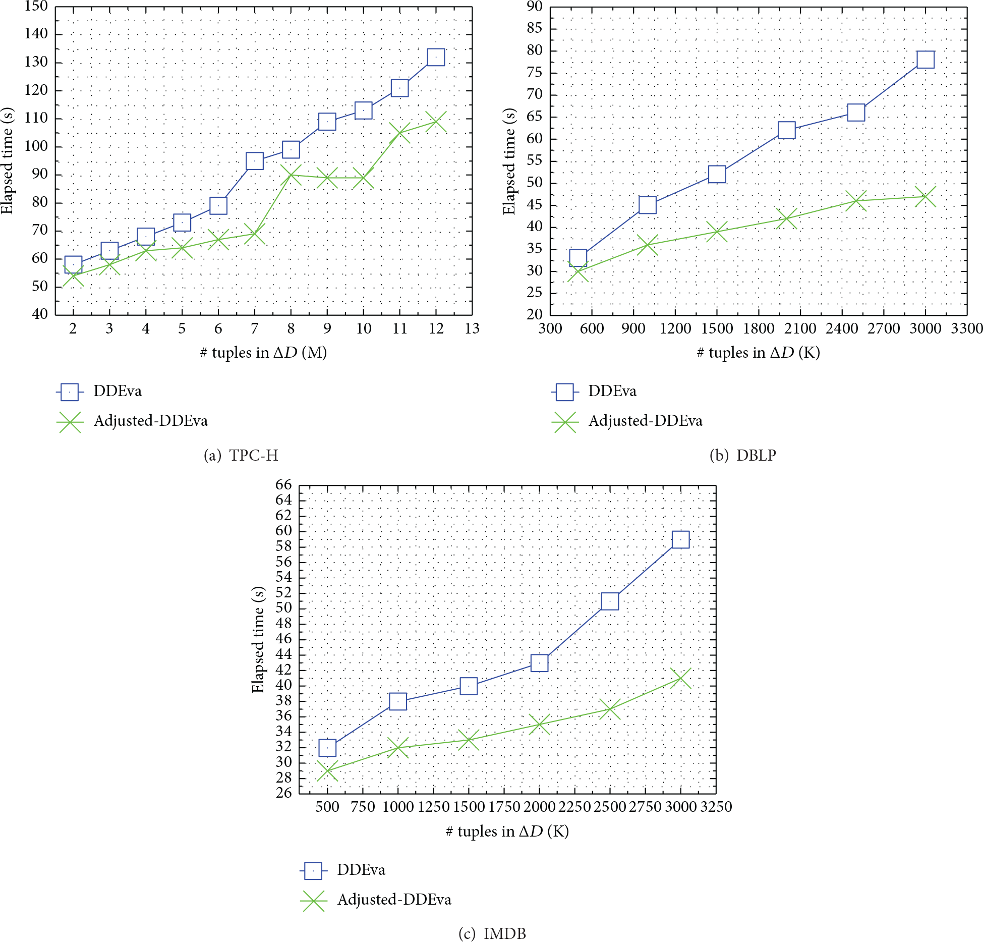
Exp-2: Impact of $\left|\Delta D\right|$ . In the second set of experiments, we show how the size of changes $\left|\Delta D\right|$ to the database affects the performance of inconsistency evaluation algorithm. Fixing $\left|\Sigma \right|=\mathrm{50}$ and $\left|D\right|=\mathrm{2}$  M, the size of $\left|\Delta D\right|$ is varied from $\mathrm{2}$  M to $\mathrm{10}$  M tuples for TPC-H. $\left|\Delta D\right|$ is varied from $\mathrm{500}$  K to $\mathrm{3000}$  K tuples for DBLP and IMDB while fixing $\left|D\right|=\mathrm{500}$  K and $\left|\Sigma \right|=\mathrm{16}$ . The elapsed times in seconds when varying $\left|\Delta D\right|$ for TPC-H (resp., DBLP and IMDB) are shown in Figure 11(a) (resp., Figures 11(b) and 11(c)).

Figure 11

Elapsed time of $DDEva$ and adjusted-DDEva.

As shown in Figures 11(a), 11(b), and 11(c), the elapsed times of adjusted-DDEva scale well up with $\left|\Delta D\right|$ , for example, $\mathrm{55}$ seconds when $\left|D\right|$ is updated from $\mathrm{2}$  M to $\mathrm{4}$  M and $\mathrm{110}$ seconds when $\left|\Delta D\right|$ is updated from $\mathrm{8}$  M to $\mathrm{10}$  M as shown in Figure 11(a).

Also, adjusted-DDEva updates the result much more efficiently than DDEva in both real-life datasets and it has a slower growth in contrast to DDEva. That is, in experiment 2, the results have shown that adjusted-DDEva updates the result much more efficiently than DDEva in both real-life datasets.

Exp-3: Impact of $\mathbf{\left|}\Sigma \mathbf{\right|}$ . In this set of experiments, we study the impact of the number of variable CFDs on data dirtiness evaluation. Fixing $\left|D\right|=\mathrm{2}$  M and $\left|\Delta D\right|=\mathrm{10}$  M for TPC-H, we varied the number of CFDs $\left|\Sigma \right|$ from $\mathrm{20}$ to $\mathrm{100}$ including $\mathrm{5}\%$ FDs. Moreover, fixing $\left|D\right|=\mathrm{500}$  K and $\left|\Delta D\right|=\mathrm{2000}$  K for DBLP and IMDB, we varied $\left|\Sigma \right|$ from $\mathrm{8}$ to $\mathrm{20}$ including $\mathrm{3}$ FDs. The elapsed times when varying $\left|\Sigma \right|$ from $\mathrm{20}$ to $\mathrm{100}$ for TPC-H (resp., from $\mathrm{8}$ to $\mathrm{20}$ for DBLP and IMDB) are shown in Figure 12(a) (resp., Figures 12(b) and 12(c)). Both $DDEva$ and $adjusted$ - $DDEva$ are able to evaluate the data dirtiness with good scalability when varying $\left|\Sigma \right|$ .

Figure 12

Elapsed time of $DDEva$ and adjusted-DDEva.

As the number of indexes will increase with $\left|\Sigma \right|$ , the elapsed time of DDEva will increase with $\left|\Sigma \right|$ . However, the elapsed time of adjusted-DDEva performance is better than that of DDEva since the size of indexes with higher rank is very small after adjusting the processing order of CFDs in Σ . The results demonstrate that adjusted-DDEva has good scalability with $\left|\Sigma \right|$ , and it works well on a larger number of CFDs.

Note that, in Figures 12(b) and 12(c), we can see that the increase of size $\left|\Sigma \right|$ does not lead to a fast growth of the adjusted-DDEva; that is really because the number of FDs included in the CFD set for DBLP and IMDB is fixed and captures most conflicts so that a large amount of random I/Os in the following indexes is prevented in practice.

Exp-4: Space Cost. In this set of experiments, we study the sizes of indexes that our algorithm needs to build. Fixing the number of general CFDs $\left|\Sigma \right|=\mathrm{5}$ , each with $\mathrm{200}$ pattern tuples generated randomly, and setting $\left|D\right|$ as $\mathrm{10}$  M for TPC-H (i.e., $\mathrm{10}$  GB) and $\mathrm{4}$  M for DBLP and IMDB (about $\mathrm{1}$  GB), we record the size of each index for the three datasets. The results are shown in Figure 13.

Figure 13

Space cost of $DDEva$ and adjusted-DDEva.

First, for each dataset, the index size decreases with the processing order; this is consistent with the definition of ir-subgraph. Second, the total space our algorithm takes does not depend on the width of the dataset due to key compression. Actually, in practice, a pair of 32-bit or 64-bit integers is enough to partition the dataset according to the values on X and Y without errors. Third, as shown in the results of this experiment, $adjusted$ - $DDEva$ takes less total space cost than its counterpart, and the first few indexes almost cover most of the matched tuples.

Exp-5: Quality of Evaluation Result. In the last set of experiments, we study the evaluation result quality of our evaluation method based on minimum culprit with respect to CFD set Σ (MC), in contrast with naïve methods based on conflicts counting (CC). Here, we introduce a variable “ ${\sigma }_{i,i-\mathrm{1}}$ ” representing the difference of data inconsistency between the ith update and the $\left(i-\mathrm{1}\right)$ th update; concretely, $(1)$ “ ${\sigma }_{i,i-\mathrm{1}}^{\mathrm{M}\mathrm{C}}$ ” is the difference of minimum culprit size estimated with respect to CFD set Σ; $(2)$ “ ${\sigma }_{i,i-\mathrm{1}}^{\mathrm{C}\mathrm{C}}$ ” is the difference of conflicts detected, respectively. To measure the result quality of two evaluation methods under assumption in $(1)$ , we compute the standard deviation of “ ${\sigma }_{i,i-\mathrm{1}}$ ” on $\mathrm{5}$ samples with $\mathrm{100}$ tuples which lead to inconsistency.

Figure 14 shows the standard deviation of variable “ ${\sigma }_{i,i-\mathrm{1}}$ ” computed for TPC-H ( $D=\mathrm{2}$  M, $\left|\Sigma \right|=\mathrm{100}$ , and $\left|\Delta D\right|$ is varied from $\mathrm{1}$  M to $\mathrm{5}$  M including only insert operation) and DBLP and IMDB ( $D=\mathrm{500}$  K, $\left|\Sigma \right|=20$ , and $\left|\Delta D\right|$ is varied from $\mathrm{500}$  K to $\mathrm{2000}$  K including only insert operation).

Figure 14

Elapsed time of $DDEva$ and adjusted-DDEva.

The figure tells us that, for each dataset, ${\sigma }_{i,i-\mathrm{1}}^{\mathrm{M}\mathrm{C}}$ is insensitive to a single update operation, but ${\sigma }_{i,i-\mathrm{1}}^{\mathrm{C}\mathrm{C}}$ is very sensitive to each single update operation which will be inconsistent with existing tuples. That is to say, the evaluation method MC studied in this paper will give a very smooth monitoring curve rather than the naïve method CC.

7.4. Summary

We find the following conclusions from the results of the experiments conducted on both synthetic data TPC-H and real-life data DBLP and IMDB. $(1)$ Our evaluation algorithms scale well with respect to the size of database $\left|D\right|$ , the size of changes to database $\left|\Delta D\right|$ , and the number of CFDs $\left|\Sigma \right|$ for large data (Exp-1 to Exp-3). $(2)$ The modified version of algorithm adjusted-DDEva outperforms its counterpart DDEva much more especially for both real-life datasets and larger $\left|\Sigma \right|$ because a few CFDs in Σ have small confidence while the others do not. $(3)$ The evaluation method proposed based on minimum culprit with respect to CFD set Σ substantially revealed how dirty the data is under the typical assumption: “ $(1)$ most of the data is often correct, especially for large data, and $(2)$ an update of a tuple with error has a very tiny impact on the dirtiness of the entire dataset” (Exp-5).

8. Related Works

Conditional functional dependency (CFD) was first proposed by the authors of [16] while the SQL techniques they provided have been applied in data cleaning broadly, which can be used to detect the inconsistencies of databases. However, there is no existing work focusing on computing the inconsistency of a database based on CFDs efficiently. The most relevant works to this paper can be categorized into inconsistency detection and resolution.

For inconsistency detection, there exist some detection techniques which are able to detect errors efficiently; SQL techniques for detecting CFD violations were given by [18]; practical algorithms for detecting violations of CFDs in fragmented and distributed relations were provided by [19] and an incremental detection algorithm was proposed by [20]. In contrast to inconsistency detection, inconsistency evaluation needs to compute the quantized dirtiness value of the data, rather than finding all violations.

For data repair, there are two kinds of works which are based on FDs/CFDs; they both aim to directly resolve the inconsistency of database. One kind of method is to repair data based on minimizing the repair cost, for example, [22, 24, 29, 36, 37]. Given the data edit operations (including tuple-level and cell-level), minimum cost repair will output repaired data with minimizing the difference between it and the original one. Our problem can be seen as a special case of [29], because the complementary minimum culprit can be seen as C-repair (cardinality repair) of an inconsistent database; however, it is much more expensive using the techniques of the authors of [27] directly, especially for dynamic data, and the algorithm given in this paper is more efficient and seems optimal. There are some other repair definitions, such as “minimum description length (MDL)” [23] and “relative trust” [21]. To the best of our knowledge, there is almost no polynomial approximation algorithm with a good ratio bound for repairing inconsistent data based on CFDs except for a few approximation algorithms with constant ratio which were provided, such as [25], while the ratio could not reach $\mathrm{2}$ , although the repair algorithm starts to need an approximate minimum vertex cover in a conflict graph, which is why they do not consider how to compute it efficiently; moreover, they cannot deal with large dynamic data well because it starts by finding all FD violations and a conflict hypergraph with respect to all FDs/CFDs should be built first which may take quadratic time and space. Another kind of method is consistent query answer (CQA) [29, 36, 38–43]; for a fixed boolean query q, $\mathrm{C}\mathrm{Q}\mathrm{A}(q)$ is the following problem: given a database D, decide whether q evaluates to true on every repair of D. Such method will not edit the data but will find a query answer among all possible repairs of original database, and, unfortunately, there is no technique in CQA that can be used in this paper directly. Moreover, there are some works considering the theoretical result of CQA under C-repair [38, 44–46], but they do not provide the technique able to solve the problem this paper studied. Additionally, if the minimality assumption fails or there are multiple optimal repairs of the data, output of repair approximation algorithm will be meaningless sometimes even if it has an accuracy guarantee. In contrast to data repair, this paper aims to output the value of dirtiness for data quality evaluation, monitoring, and so on. Therefore, approximation with constant factor is also the lower bound of repairing cost.

9. Conclusions

This paper studied the data consistency evaluation based on CFDs, in order to give a quantized quality value to users. We proved that the complexity of dirtiness evaluation is NP-complete even if the condition is simple enough; moreover, for any $\epsilon >\mathrm{0}$ , it is hard to give an approximation within $\mathrm{2}-\epsilon$ in polynomial time. The time complexity of our $\mathrm{2}$ -approximate algorithm is $O\left(n\log n\right)$ , and it scales well. To deal with the larger data and its update, the compact structure reduces the storage of conflict graph to $O\left(rn\right)$ and reduces the time of update to $O\left(r\log n\right)$ . The experiments show that our algorithm scales well with data size and the quality of its evaluation result is good.