Human Mobility Prediction Based on Social Media with Complex Event Processing

Abstract

The combination of mobile and social media sensors is foreseen to become a crucial course of action so as to comprehensively capture and understand the movement of people in large spatial regions. In that sense, the present work describes a novel personal location predictor that makes use of these two types of sensors. Firstly, it extracts the mobility models of an area capturing aspects related to particular users along with crowd-based features on the basis of geotagged tweets. Unlike previous approaches, the proposed solution mines such models in an online manner so that no previous off-line training is required. Then, on the basis of such models, a predictor able to forecast the next activity and position of a user is developed. Finally, the described approach is tested by using Twitter datasets from two different cities.

1. Introduction

Nowadays, handheld and wearable devices have actually become instrumental tools for most of our daily tasks. Among other features, such devices have been steadily enriched with more precise positioning sensors, like GPS. This has allowed collecting a large amount of high-resolution digital traces which, in turn, have eased the development of the mobility mining discipline which focuses on giving insight into the underlying spatiotemporal trajectories of the gathered traces [1]. As a result, innovative location-based services have been developed like personal advertisement campaigns [2] or pervasive navigation systems [3].

At the same time, social networking has become a very popular activity in most developed and developing societies allowing people to remain socially connected to their friends, relatives, and colleagues in an easy manner. As a matter of fact, the number of active users of social media reached 2000 million in August 2014 (http://wearesocial.net/blog/2014/08/global-social-media-users-pass-2-billion/).

During recent years, many social network and microblogging sites, such as Twitter, Facebook, or Foursquare, have included location-based capabilities into their smartphone's applications. The fact that most of the documents and data belonging to those sites can be geotagged thanks to these capabilities has enabled the advent of what has been called soft sensors combining social media and location data.

From these soft sensors, an unprecedented amount of user-generated data on human movement and activity participation has become easily available. Unlike previous mobility datasets (e.g., GPS-based ones), these new ones not only include spatiotemporal information (e.g., the spatial coordinates of a person at a particular moment) but also include textual data attached to a particular spot which provides more semantic information.

In this scope, a new course of action within the aforementioned mobility mining discipline focuses on giving insight into this new social media data so as to come up with novel human mobility models and patterns [4–6]. Nonetheless, previous studies frequently suffer from some of the following limitations:

• (i)

They center on extracting general mobility information related to a particular urban area or region without distinguishing between particular users. In that sense, inferring more personal mobility models might be useful to come up with more customized location services.

(ii)

A preprocessing step of the whole available dataset is required before generating the final models or patterns. However, under certain conditions, this requirement is not feasible as the whole dataset is not available in advance.

(iii)

Moreover, most works constrain their processing to the spatiotemporal aspects of the data (check-in posts) without considering other textual details like the content of the document. As a result, these works do not fully take advantage of social media datasets.

(iv)

Lastly, little efforts have been done so far to devise solutions able to anticipate future locations or activities of users, by taking advantage of geotagged social media documents.

In this context, the present work puts forward a novel approach for personal mobility mining based on microblogging content that fully considers the four limitations listed above.

In particular, the proposed system composes personal mobility graphs in an online fashion. A user's personal graph is endlessly generated and updated on the basis of his geotagged documents (“tweets”) gathered on the social network Twitter (https://twitter.com/). Next, such graphs are steadily aggregated to compose a hierarchy representing the mobility flows of a large spatial region.

Unlike previous approaches, these graphs include the important geographical areas of a person or region (“landmarks”), how they are interconnected, and also the frequent topics mentioned in Twitter within each place by considering not only check-in documents.

Figure 1 depicts an illustrative example of the aforementioned mobility graph hierarchy which basically comprises two different levels. The first one is compound of the personal graphs related to particular users, whereas the second level comprises a more general one representing the crowd-based mobility within the spatial region of interest.

Figure 1

Overview of the proposal.

In order to compose each graph, three key mechanisms have been used, a novel density-based clustering for the extraction of meaningful places, whereas the topic mining has been carried out by means of lightweight bag of words solution. In addition to that, due to the event nature of tweets, the orchestration of all the components has been done with the Complex Event Processing (CEP) paradigm [7]. CEP is a well-established technology to extract predefined patterns in event-based environments.

Next, on the basis of the historical data contained in the whole graph hierarchy, a multilevel Markov-model-based predictor has been designed. In brief, it incrementally accesses each graph level until a suitable prediction is generated regarding location and potential activity. In that sense, the prediction is also discretized considering temporal factors.

Last but no least, the adopted solution takes the form of a mobile client and a back-end server. The client runs and deals with personal mobility features whereas the back-end server is in charge of the crowd-sensing features.

To sum up, bearing in mind the four current limitations for mobility mining based on social media previously listed, the salient contributions of the present work can be summarized as follows: (1) a novel mobility model based on Twitter data that considers both personal and crowd-based mobility, (2) an online approach to extract such a model with no need of off-line processing, (3) the usage of different types of geotagged documents and not only check-in ones, and (4) one of the first attempts to anticipate future user's location by only relying on social media information.

The remainder of the paper is structured as follows. An overview of the approach's background is put forward in Section 2. Section 3 is devoted to describing the logic structure of the proposed system. Then, Section 4 shows a study of the proposal. Finally, the main conclusions and the future work are summed up in Section 5.

2. Related Work

An overview of the contribution of our work with respect to related domains is stated in this section.

2.1. Social Media for Human Mobility

During recent years, data from several social network sites has been mainly used to extract information related to different types of human features. Apart from sentiment analysis [8, 9], a foremost line of research in this domain focuses on mining useful information related to how people move and the underlying goals of this movement. In that sense, it is possible to classify these works under three different categories.

Firstly, one group of works aim at automatically extracting spatial regions within an urban area on the basis of their usage (e.g., leisure, home, and work) by processing geotagged tweets [6, 10, 11]. For that goal, either visual analytics [11] clustering algorithms [10] or predefine classifiers from third-party location services [6] are commonly used to process the data coming from social network sites.

Secondly, another course of action intends to automatically extract events of interest (e.g., live shows, exhibitions, and traffic jams) from social media. For instance, [12, 13] come up with smart social agendas that can be updated in real time whereas [14] makes use of tweets so as to timely detect potential earthquakes. In a road-traffic monitoring scenario, several works make use of social media data in order to either detect or semantically enrich traffic anomalies. This is the case of [15], which studies the correlation between tweets and road-traffic incidents. [16] takes social media data as input in order to explain previously detected traffic problems. Similarly, [17] collects documents from official traffic-management institutions' Twitter accounts in order to detect in real time traffic congestions.

Finally, our work is enclosed in a third line of study whose main goal is to include social media as a new data-source for detecting the movement of different kinds of people among different places [4–6, 18]. More in detail, [4] proposes a novel approach to semantically enrich spatiotemporal trajectories given data from different social media sites. This way, a more dynamic labelling is achieved. Moreover, [18] states a worldwide mobility report based geotagged Twitter data. Apart from that, [6] proposes a personal mobility mining approach to detect the frequency in which a user visits different locations on the basis of his underlaying activity. Finally, [5] processes the spatial coordinates of geotagged tweets in order to compose the spatial-temporal trajectories of a set of Twitter users. Such trajectories are defined as simple Origin-Destination matrices and the labelling of each potential origin or destination is done by means of a third-party location service.

Despite some similarities between the aforementioned solutions and our work, some key differences can also be stated. In that sense, either such works rely on previously collected datasets or, even providing real time processing, all this processing is centralized in a back-end server without providing any component running in the clients' mobile devices. In addition to that, works like [4, 6] do not use regular social media documents as incoming data but only check-in documents. These types of documents explicitly indicate when the user has been at a certain venue by appending a URL providing more details of such a venue. A clear example of social site that provides this type of content is Foursquare (https://foursquare.com/).

On the contrary, our proposal defines a proper client-server architecture able to run in smartphones. Furthermore, the solution also avoids a preprocessing step of the dataset by incrementally composing the graphs. Finally, the system has been designed to take as input regular tweets, not only check-in ones.

2.2. Location Prediction

Location prediction is based on the assumption that common people follow daily routines and, thus, have only a set of frequently visited locations [19]. This makes people's regular trips quite predictable due to their high level of repetition [20, 21].

In this scope, it is possible to mainly distinguish two different trends for personal location prediction. The former follows a geometrical approach so as to predict a path in the Euclidean space [22, 23]. In this line of work, future locations are predicted by applying a mathematical function to the current location and velocity of the target person.

The second line of work is based on pattern matching and it profits from the above-mentioned repetition assumption. In brief, solutions within this trend compare the route in progress with a set of mobility models (created on the basis of previously observed routes). If a match fires, the selected (group of) pattern(s) is used to make a prediction [24]. In that sense, Bayesian networks [25, 26], hidden Markov models [27–30], and Markov decision processes [31] have been some of the applied solutions given high-resolution mobility datasets (e.g., those comprising GPS-based traces). Despite the fact that these datasets provide more detailed mobility information, they are not really convenient for full-blown deployments as GPS feed is one of the most battery-draining sensors of a mobile device. On the contrary, our work relies on social media sources that are not so expensive in terms of energy usage as the aforementioned positioning sensors.

Regarding social media datasets, a remarkable solution for location prediction is the probabilistic model W⁴ described in [32]. By following a Bayesian-network approach, the proposed system is able to forecast the next location and activity of a user by also taking into account temporal factors. Despite the fact that the goal of such a method and our work is the same, a major difference exists. W⁴ makes up a Bayesian-network for each single user by only using his own tweets. Similarly, our work also composes a set of personal graphs by only using the geotagged tweets of the target user. Nonetheless, it also creates a mobility graph combining the tweets from all users representing the crowd-dynamics within a region. Then, both types of graphs are used to provide a prediction. Therefore, unlike W⁴, our system makes use of personal and more general mobility information to provide prediction.

Lastly, [33] provides a complete analysis of which mobility features may have an impact on next location prediction given social media diaries. Despite its interesting results, authors focus on check-in documents instead of other types of social media content.

2.3. Complex Event Processing

Complex Event Processing (CEP) is an evolution of the former publish/subscribe model in order to deal with more complex subscription patterns, so it can be regarded as a relatively recent technology [7].

Despite CEP's widespread usage, there exists a scarcity of CEP solutions which deal with spatiotemporality since only a few works actually propose practical CEP applications able to process spatiotemporal data [34]. In that sense, [35] devises a formal framework to timely detect spatiotemporal relationships between moving entities. However, such a solution only focuses on GPS-based high-resolution data discarding other types of spatiotemporal event sources.

Concerning the usage of CEP to process events generated by social network sites, only theoretical solutions to define formal event-based information models and architectures for social media processing have been put forward so far [36]. Therefore, to the best of the authors knowledge, this paper constitutes one of the first efforts to actually process social media data by means of the CEP paradigm.

3. Proposed System

This section is devoted to explain in detail the goal along with the architecture of the proposal.

3.1. Prediction Target

The main goal of the present system is to provide an accurate and early prediction of the next meaningful location, or landmark, visited by a person along with the underlying activity of such a place.

As the bottom of Figure 1 shows, we assume that the spatial and temporal spread of tweets of a user define a set of personal landmarks like his home, office, school, and so forth. In our setting, such landmarks have been defined by means of a spatial approach.

Definition 1.

A landmark for a person $\mathcal{P}$ , ${\mathcal{L}}_p$ , is a spatial region frequently visited by $\mathcal{P}$ , where he tends to share his thoughts, activities, or other interests by means of tweets.

Furthermore, the spatial and temporal distribution of tweets also composes a set of more general landmarks that are not related to a particular individual but, instead, are meaningful for a crowd of people, like the center of a city, business parks, or shopping areas. Such collective landmarks can be defined as follows.

Definition 2.

A collective landmark, ${\mathcal{L}}_c$ , is a spatial region frequently visited by more than one individual where they tend to share their thoughts, activities, or other interests by means of tweets.

Consequently, from a social media point of view, the mobility of a person is constrained to personal and collective landmarks. In this way, the route of a person can be stated as follows.

Definition 3.

A route of a person $\mathcal{P}$ , ${\mathcal{R}}_p$ , is a sequence ${\mathcal{R}}_p^s=\{{\mathcal{L}}_{\mathrm{1}},\dots ,{\mathcal{L}}_{\mathrm{1}+n}\}$ ( $n\ge \mathrm{1}$ ) of personal or collective landmarks $\mathcal{L}$ visited by $\mathcal{P}$ during a time interval $\mathcal{T}$ .

All in all, our approach focuses on predicting the next personal or crowd-based landmark $\mathcal{L}$ within a route ${\mathcal{R}}_p$ , at the same time it is being covered. This prediction is initiated when the person departs from ${\mathcal{L}}_{\mathrm{1}}$ , and it is updated in real time while new landmarks are added to the route's sequence ${\mathcal{R}}_p^s$ .

3.2. Architecture Overview

In order to achieve the prediction features explained before, the present system has been designed to run in handheld devices. Nonetheless, due to the different types of landmarks to be detected, the system architecture has been split into two parts, a client side that runs on the mobile device of each user in charge of detecting personal landmarks and a server side responsible for composing the collective ones.

The system's logic structure is depicted in Figure 2. For its design, the CEP paradigm has been followed. Thus, the system's inner structure basically consists of a palette of interconnected Event Processing Rules (EPRs) along with other modules providing different kinds of computational support.

Figure 2

System architecture. The components that are not EPRs are depicted as dashed boxes.

Each EPR takes as input one or more streams of raw or derived streams. From these streams, it is in charge of detecting a specific pattern. Each time EPR fires, a derived event is composed and asynchronously distributed to other upstream EPRs or an event sink or consumer.

3.3. Event Model

When it comes to develop a CEP system, one of the first tasks to be undertaken is the definition of the events that the system is going to make up during its execution. In this scope, Figure 3 depicts the information model of the system. As we can see from it, the event types have been structured by means of a hierarchical approach.

Figure 3

Information model of the system.

On the one hand, the tweet event represents a raw tweet written by the user. In that sense, the attributes of this event include not only the textual content of the tweet but also other important metadata like the user nick, its timestamp, and its geotagging. Next, the tweet with topic event refines it by including the most probable topics its textual content refers to.

On the other hand, landmark event further enhances the previous tweet events by also indicating if a tweet has been written inside any personal or collective landmark. Finally, the route event represents a completed route as a sequence of personal or collective landmarks as it was put forward in Definition 3.

Most route prediction approaches usually consist of a chained process comprising three stages, route composition, mobility model generation, and eventually location prediction. Therefore, the description of the system is split into these three steps.

3.4. Route Composition

This first step aims at composing the ongoing route ${\mathcal{R}}_p$ of each user $\mathcal{P}$ at the same time he writes geotagged tweets. For that goal, the four EPRs enclosed in the mobile client are involved to achieve this online composition (see Figure 2).

3.4.1. Tweet Filter EPR

First of all, this rule is in charge of filtering out the incoming user's tweets that might not provide useful information to infer his current activity. In that sense, this rule discards those tweets that are just repetitions (“retweets”) of a tweet written by a completely different user. This way, we ensure that the route will be composed of the documents originally written by the user.

Moreover, this event rule also undertakes the cleaning of the text content of the tweet. In that sense, elements that do not provide information about the user's current activity are considered as noise and, hence, removed from the text. Such elements are (1) URL links, (2) mentions to other users, and (3) stop words, including articles and pronouns.

An event-based processing rule generally comprises two different parts, (1) a condition part where the requirements for the rule to fire are listed and (2) an action part that indicates the actions to be done if the condition part is fulfilled. Consequently, the pseudocode of the tweet filter EPR looks as follows:

•  

CONDITION

•  

RawTweet AS t AND NOT t.text.contains(＇＇RT:  ＇＇)

 

ACTION

•  

new TweetEvent(t.user, t.timestamp, t.location, clean_text(t.text))

where the string ＇＇RT:  ＇＇ is the default prefix indicating a retweeted content and the clean_text function is responsible for the text cleaning process.

3.4.2. Tweet Topic EPR

The next step in the route composition is to detect which is the underling activity that each filtered tweet refers to, if any. For that goal, an approach based on a bag of words has been applied. This involves two different tasks.

To begin with, it is necessary to define a set $\mathcal{A}$ of target activities to be detected. In our setting, we defined a taxonomy of the most remarkable daily activities of a person. It is initially based on concept of activities of daily living from the healthcare domain [37] and the ontology for activities in indoor smart environments proposed in [38]. From these sources, it is possible to distinguish between two types of activities, (1) basic activities that a person usually performs on his own without any kind of cooperation with other people and (2) activities that a person can or cannot perform in conjunction/cooperation with a community. Bearing this dichotomy in mind, we defined a complete taxonomy of target activities comprising 82 topics in 5 different levels of granularity. Figure 4 depicts a simplified version of the taxonomy whereas Figures 24 and 25 in the Appendix show the complete one.

Figure 4

Simplified taxonomy of target activities.

Secondly a bag of key unigrams ${\mathcal{B}}_a$ with high correlation to each activity $a\in \mathcal{A}$ is composed. In that sense, the particular unigram set of each activity strongly depends on the particular scenario of deployment (e.g., the language of the target users, their urban environment). In that sense, Section 4 describes the generated bags of unigrams for the evaluated scenarios.

Next, the tweet topic EPR makes use of the aforementioned bags of words for the activity discovery procedure. To do so, it matches the keywords of each new tweet event t with the bag of words ${\mathcal{B}}_a$ of each activity $a\in \mathcal{A}$ . If any of the keywords of t is contained in ${\mathcal{B}}_a$ , then a is included in the set ${\mathcal{A}}_t\subseteq \mathcal{A}$ of activities mentioned in the tweet t. Note that at the end of the procedure ${\mathcal{A}}_t$ might be empty if there is not any match between the keywords and all the bags of words. As a result, a new tweet with topic event comprising ${\mathcal{A}}_t$ is generated. For the sake of completeness, the pseudocode of the rule is shown next:

•  

CONDITION

•  

TweetEvent AS t

 

ACTION

•  

new TweetWithTopicEvent(t.user, t. timestamp, t.location, t.text, find_ activities(t.text))

where the function find_activities represents the activity detection described above. Note that this function could return an empty set indicating that there have not been any match.

3.4.3. Tweet in Landmark EPR

Once the activity discovery has been done, the next step in the route composition stage is to detect the landmark $\mathcal{L}$ comprising each new tweet with topic event. As the information model in Figure 3 shows, a landmark comprises two features, its covered spatial region and the list of activities frequently associated with such a region.

Regarding the landmark's spatial region, if we consider Definitions 1 and 2, personal and collective landmarks can be regarded as spatial regions with a high density of tweets related to one or more activities. As a result, a density-based clustering has been applied to tweets' locations for landmark detection. This type of clustering has been widely applied to detect meaningful places given sets of spatiotemporal trajectories as in [39].

In short, density-based clustering is based on the concept of local neighbourhood $\mathcal{N}$ of a point p, that is, the number of points that are within a certain straight distance Eps to p:

$$\begin{array}{cc}& \mathcal{N}\left(p\right)=\left\{q\in \mathcal{S}\mid \mathrm{d}\mathrm{i}\mathrm{s}\mathrm{t}\left(p,q\right)\le Eps\right\},\end{array}$$

(1)

where $\mathcal{S}$ is the set of available points. If $|\mathcal{N}(p)|$ is over a certain threshold $MinPoints$ , then $\mathcal{N}(p)$ is considered a cluster. Furthermore, $\mathcal{N}(p)$ is density-joinable to $\mathcal{N}(q)$ ( $p\ne q$ ) if $\mathcal{N}(p)\cap \mathcal{N}(q)\ne \varnothing$ .

The density clustering algorithm applied for landmark detection is a slightly modified version of the online landmark discovery algorithm (LDM) described in [40].

In brief, LDA firstly intends to detect the set of centroids $\mathcal{C}$ from the received points $\mathcal{S}$ , where $\mathcal{C}=\{c_{\mathrm{1}},c_{\mathrm{2}},\dots ,c_n\}\subset \mathcal{S}$ and

• (i)

$|\mathcal{N}(c_i)|\ge MinPoints\hspace{0.17em}\hspace{0.17em}\forall c_i\in \mathcal{C}$ ,

(ii)

$\mathrm{d}\mathrm{i}\mathrm{s}\mathrm{t}(c_i,c_j)>Eps,\hspace{0.17em}\hspace{0.17em}i\ne j\hspace{0.17em}\hspace{0.17em}\forall c_i,c_j\in \mathcal{C}$ .

On the basis of the detected centroids, a landmark $\mathcal{L}$ is defined as a group of centroids where the neighbourhood of each centroid is density-joinable with the neighbourhood of at least another centroid in the same landmark as Figure 5 illustrates. Therefore, the LDM basically returns, given a point p, the landmark $\mathcal{L}$ of the centroid c whose neighbourhood $\mathcal{N}(c)$ comprises p, if any. At the same time, it also detects the different centroids and landmarks.

Figure 5

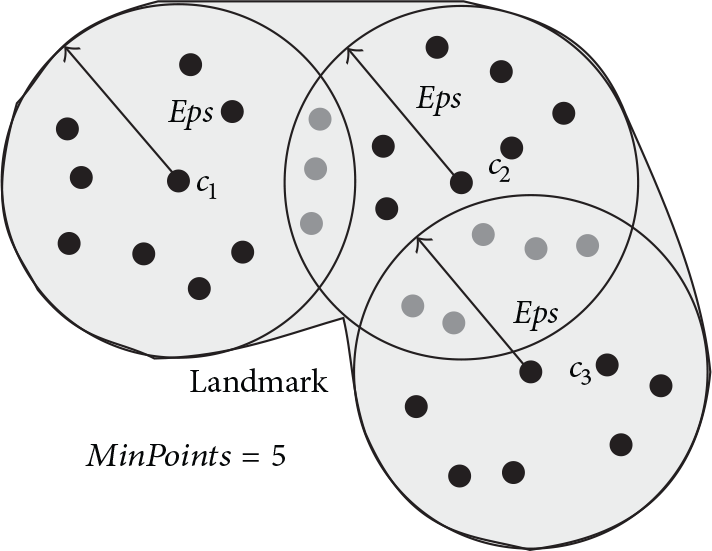
Example of a landmark returned by the LDA.

For the present work, the original algorithm has been adapted to certain characteristics of the present setting such as the spatial distribution of tweets and the fact that the client side is intended to run in handheld contrivances that should be regarded as memory-constrained devices.

Regarding the memory saving improvement, unlike the previous version of LDA, the set of available points $\mathcal{S}$ only comprises the tweet locations that are not assigned to any landmark yet along with the detected centroids instead of all the locations collected so far. For example, given the situation depicted by Figure 6, $\mathcal{N}(p_{\mathrm{7}})$ comprises the locations $p_{\mathrm{1}}$ , $p_{\mathrm{2}}$ , $p_{\mathrm{3}}$ , and $c_{\mathrm{1}}$ as locations $p_{\mathrm{4}}$ , $p_{\mathrm{5}}$ , and $p_{\mathrm{6}}$ are already assigned to landmark ${\mathcal{L}}_{\mathrm{1}}$ . The reason for this mechanism is that a location, which is not a centroid, becomes useless in the original LDA once it is included in the local neighbourhood $\mathcal{N}$ of a centroid. Therefore, it is not really necessary to keep these locations in disk.

Figure 6

Example of local neighbourhood $\mathcal{N}$ given the restricted content of $\mathcal{S}$ . The locations actually contained in $\mathcal{N}(p_{\mathrm{7}})$ are shown in orange.

Concerning the algorithm itself, it basically comprises two steps. In the first one (lines 4–10 of Algorithm 1), the algorithm tries to detect whether the incoming tweet t is already within the neighbourhood of any existing centroid. This step has been modified in order to avoid the spatial overspread of landmarks in the original approach. This caused the landmarks to cover very large spatial regions. In the present work, very large landmarks are not really convenient. The larger a landmark is, the more varied types of activities might be assigned to it. In our case, it is desirable to keep the types of activities associated with a more concise landmark.

Algorithm 1: The tweet-based landmark discovery algorithm.

Input: A tweet t.

Output: The Landmark region l containing p, if any.

(1)  $l\leftarrow \mathrm{\varnothing }$

(2)  $p\leftarrow t.location$

(3)  $p.user\leftarrow t.user$

(4) for each   $q\in \mathcal{N}(p)$   do

(5)   if   $q\in \mathcal{C}$   then

(6)     if   $p.centroid=null$   then

(7)       if   $\mathrm{d}\mathrm{i}\mathrm{s}\mathrm{t}(p,\zeta (q.landmark)\le Eps$ )  then

(8)          $l\leftarrow q.\mathrm{l}\mathrm{a}\mathrm{n}\mathrm{d}\mathrm{m}\mathrm{a}\mathrm{r}\mathrm{k}$

(9)     else if

       $\mathrm{d}\mathrm{i}\mathrm{s}\mathrm{t}(\zeta (l),\zeta (q.landmark)\le Eps\times f_{overlap}$ )

      then

(10)        $l\leftarrow \mathrm{M}\mathrm{e}\mathrm{r}\mathrm{g}\mathrm{e}(l,q.\mathrm{l}\mathrm{a}\mathrm{n}\mathrm{d}\mathrm{m}\mathrm{a}\mathrm{r}\mathrm{k})$

(11) if   $l=\mathrm{\varnothing }$   then

(12)   if   $\left|\mathcal{N}\left(p\right)\right|$  ≥  $MinPoints$   then

(13)      $\mathcal{C}\leftarrow \mathcal{C}\mathcal{}\mathcal{}\cup p$

(14)      $l\leftarrow \mathrm{n}\mathrm{e}\mathrm{w}\_\mathrm{l}\mathrm{a}\mathrm{n}\mathrm{d}\mathrm{m}\mathrm{a}\mathrm{r}\mathrm{k}(p)$

(15)      $l.\mathrm{i}\mathrm{s}\_\mathrm{n}\mathrm{e}\mathrm{w}\leftarrow \mathrm{t}\mathrm{r}\mathrm{u}\mathrm{e}$

(16)     for each   $q\in \mathcal{N}$ (p)  do

(17)       if   $q\in \mathcal{C}$   then

(18)         if   $\mathrm{d}\mathrm{i}\mathrm{s}\mathrm{t}(p,\zeta (q.landmark)\le Eps\times f_{overlap})$   then

(19)            $l\leftarrow \mathrm{M}\mathrm{e}\mathrm{r}\mathrm{g}\mathrm{e}(l,q.\mathrm{l}\mathrm{a}\mathrm{n}\mathrm{d}\mathrm{m}\mathrm{a}\mathrm{r}\mathrm{k})$

(20)       else

(21)          $\mathcal{S}\leftarrow \mathcal{S}-q$

(22) if   $l=\mathrm{\varnothing }$   then

(23)    $\mathcal{S}\leftarrow \mathcal{S}\cup p$

(24) $l.topics\leftarrow t.topics$

(25) return  l

Consequently, unlike the original LDA, the tweet location p is only considered as part of a landmark $\mathcal{L}$ if the distance between p and the landmark's middle point $\zeta (\mathcal{L})$ is less than or equals Eps (line 7). An example of this step is depicted in Figure 7. While in (a) the point p will be appended as part of the landmark, the situation in (b) will not cause p to be included avoiding the spatial growth of the landmark.

Figure 7

Example of two potential situations between an incoming tweet location p and a landmark with two centroids ( $c_{\mathrm{1}},c_{\mathrm{2}}$ ). While in (a) p will be part of the landmark, in (b) this will not occur.

Moreover, in order to avoid the overmerging problem of the original LDA, two different landmarks are now merged only if the distance between its middle points is less than or equal to $Eps\times f_{overlap}$ , where $f_{overlap}\in (\mathrm{1,2}]$ is a factor which allows adjusting the required overlapping of two landmarks to be merged.

The second step (lines 11–21) is executed if the incoming tweet location p is not included in any existing centroid's neighbourhood. In that case, the algorithm first checks if p can be considered a centroid (line 12). If that condition is accomplished, a new landmark is generated (lines 14-15), it is merged with any other surroundings (lines 17–19) and the locations, which are not centroids, in $\mathcal{N}(p)$ are removed from $\mathcal{S}$ as they are now part of landmark.

Finally, the resulting landmark is tagged with the same activities associated with the incoming tweet t (line 24). In that sense, if the algorithm has not been able to detect any landmark, the incoming location p is include in $\mathcal{S}$ (lines 22-23).

Computational Complexity. Computing the neighbourhood of a point is $\mathcal{O}(n^{\mathrm{2}})$ without a spatial index and $\mathcal{O}(n\log n)$ with R-trees [41], where n is the number of stored locations and the join computation of two clusters is also $\mathcal{O}(n^{\mathrm{2}})$ without a spatial index and $\mathcal{O}(n\log n)$ with R-trees. Therefore, the complexity of the first and second step is $\mathcal{O}(n^{\mathrm{2}}\log n)\approx \mathcal{O}(n^{\mathrm{2}})$ . On the whole, the overall complexity of the algorithm is $\mathcal{O}(n^{\mathrm{2}})$ .

On the whole, two instances of the algorithm are executed (see Figure 2); the personal landmark discovery algorithm ( $\mathrm{L}\mathrm{D}{\mathrm{A}}_p$ ) locally runs in the user's device so as to detect personal landmarks. The collective landmark discovery algorithm ( $\mathrm{L}\mathrm{D}{\mathrm{A}}_c$ ) is in the back-end server for the collective landmarks. In that sense, $\mathrm{L}\mathrm{D}{\mathrm{A}}_c$ has a slight difference with respect to $\mathrm{L}\mathrm{D}{\mathrm{A}}_p$ .

Due to Definition 2, a spatial region is considered a collective landmark only if it is frequently visited by a group of different people. In order to support this characteristic, the $\mathrm{L}\mathrm{D}{\mathrm{A}}_c$ calculates the neighbourhood of a point p, $\mathcal{N}(p)$ in a slightly different manner. First of all, $\mathcal{N}(p)$ is composed as it has been explained before. Next, it is further refined by only keeping one point per user and removing the other points of the same user. Hence, we avoid the possibility that one single user gives rise to a collective landmark.

As Figure 2 the tweet in landmark EPR composes a new landmark event from each tweet with topic event by indicating the detected personal or collective landmarks. Hence, the rule code is shown next:

•  

CONDITION

•  

TweetWithTopicEvent AS t

 

ACTION

•  

new LandmarkEvent(t.user, t. timestamp, t.topic $\mathrm{L}\mathrm{D}{\mathrm{A}}_p$ (t), $\mathrm{L}\mathrm{D}{\mathrm{A}}_c$ (t) )

In that sense, if the original tweet with topic event does not have an associated topic, then this landmark event represents that the user has visited the region for an unspecified purpose.

3.4.4. Route Composer EPRs

At this point, a stream of tweet in landmark events has been generated. On the basis of the landmarks contained in these events, the ongoing route of a user ${\mathcal{R}}_p^s$ is composed.

In order to do that, the different landmarks are appended to ${\mathcal{R}}_p^s$ by following a time-based criteria. More in detail, all the landmarks ${\mathcal{L}}_i$ in ${\mathcal{R}}_p^s=\{{\mathcal{L}}_{\mathrm{1}}\cdots \to {\mathcal{L}}_i\to {\mathcal{L}}_{i+\mathrm{1}}\to \cdots {\mathcal{L}}_{\mathrm{1}+n}\}$ should accomplish two constraints:

• (i)

${\mathcal{L}}_{i+\mathrm{1}}.timestamp-{\mathcal{L}}_i.timestamp\le {\mathcal{T}}_b^{\mathrm{m}\mathrm{a}\mathrm{x}}\hspace{0.17em}\hspace{0.17em}\forall {\mathcal{L}}_i,{\mathcal{L}}_{i+\mathrm{1}}\in {\mathcal{R}}_p^s$ ,

(ii)

${\mathcal{L}}_{\mathrm{1}+n}.timestamp-{\mathcal{L}}_{\mathrm{1}}.timestamp\le {\mathcal{T}}_r^{\mathrm{m}\mathrm{a}\mathrm{x}}$ ,

where $\mathcal{L}.timestamp$ refers to the moment at which the user visited landmark $\mathcal{L}$ . The first condition imposes that two consecutive landmarks in the sequence are separated by no more than ${\mathcal{T}}_b^{\mathrm{m}\mathrm{a}\mathrm{x}}$ time units whereas the second one ensures that the time span of the whole route is not longer than ${\mathcal{T}}_r^{\mathrm{m}\mathrm{a}\mathrm{x}}$ . Thus, we ensure that all the landmarks visited by the user are somehow related in a temporal basis.

Consequently, two different EPRs are devoted to compose ${\mathcal{R}}_p^s$ at the same time the landmark events are generated. The first one fires if a landmark event fulfils the two aforementioned conditions. Hence, it is included in as a new element at the end of the ongoing ${\mathcal{R}}_p^s$ . Here is its pseudocode:

•  

CONDITION

•  

LandmarkEvent AS l AND l.timestamp - ${\mathcal{R}}_p^s$ .getLast.timestamp ≤ ${\mathcal{T}}_b^{\mathrm{m}\mathrm{a}\mathrm{x}}$ AND l. timestamp - ${\mathcal{R}}_p^s$ .getFirst.timestamp ≤ ${\mathcal{T}}_r^{\mathrm{m}\mathrm{a}\mathrm{x}}$

 

ACTION

•  

${\mathcal{R}}_p^s$ .append(l)

The second rule just mirrors the previous one to detect if the new landmark event does not belong to the current route. If so, the current route is considered as finished and a new one must be started:

•  

CONDITION

•  

LandmarkEvent AS l AND (l.timestamp - ${\mathcal{R}}_p^s$ .getLast.timestamp > ${\mathcal{T}}_b^{\mathrm{m}\mathrm{a}\mathrm{x}}$ OR l. timestamp - ${\mathcal{R}}_p^s$ .getFirst.timestamp > ${\mathcal{T}}_r^{\mathrm{m}\mathrm{a}\mathrm{x}}$ )

 

ACTION

•  

LocalGraphManager.update( ${\mathcal{R}}_p^s$ ) AND ${\mathcal{R}}_p^s$ .restartWith(l)

Furthermore, if this second rule fires, it also sends the just-completed route to the Local Graph Manager (LGM) (see Figure 2). As it will be put forward in the following section, this module carries out the update and management of the personal mobility graph in the user's device.

3.4.5. Graph Generation

This second stage of the route prediction focuses on generating on the fly the personal and collective mobility graphs, ${\mathcal{G}}_p$ and ${\mathcal{G}}_c$ . This is done on the basis of the completed routes' sequences ${\mathcal{R}}_p^s$ generated by the previous step. More in detail, both graphs encode the statistical information from the routes as a directed multigraph where each vertex represents a unique landmark.

Figure 8 shows an illustrative example of a multigraph comprising 3 different routes, ${\mathcal{R}}_p^{\mathrm{1}}=\{{\mathcal{L}}_p^{\mathrm{1}}\{meet/talk\hspace{0.17em}\hspace{0.17em}to/with\hspace{0.17em}\hspace{0.17em}others\}$ → ${\mathcal{L}}_c^{\mathrm{2}}\{go\hspace{0.17em}\hspace{0.17em}shopping\}$ → ${\mathcal{L}}_p^{\mathrm{4}}\{working\}\}$ , ${\mathcal{R}}_p^{\mathrm{2}}=\{{\mathcal{L}}_p^{\mathrm{3}}\{working\}$ → ${\mathcal{L}}_p^{\mathrm{4}}\{individual\hspace{0.17em}\hspace{0.17em}study\}$ → ${\mathcal{L}}_c^{\mathrm{2}}\{do\hspace{0.17em}\hspace{0.17em}sports\}$ → ${\mathcal{L}}_p^{\mathrm{1}}\{sleeping\}\}$ , and ${\mathcal{R}}_p^{\mathrm{3}}=\{{\mathcal{L}}_p^{\mathrm{3}}\{working\}$ → ${\mathcal{L}}_p^{\mathrm{4}}\{individual\hspace{0.17em}\hspace{0.17em}study\}$ → ${\mathcal{L}}_c^{\mathrm{5}}\{night\hspace{0.17em}\hspace{0.17em}life\}$ → ${\mathcal{L}}_p^{\mathrm{1}}$ → ${\mathcal{L}}_c^{\mathrm{2}}\}$ . As we can see, the multigraph approach allows connecting the same pair of landmarks with different directed edges where each one is labelled with the identifier and frequency of a particular route. This way, a route is encoded in $\mathcal{G}$ as a sequence of exclusive edges connecting the landmark vertices in the same order as the route. For example, the multigraph of Figure 8 indicates that route ${\mathcal{R}}_p^{\mathrm{1}}$ has been covered 12 times by the user.

Figure 8

Example of a multigraph structure. Each edge is labelled with the tuple $\{\mathrm{r}\mathrm{o}\mathrm{u}\mathrm{t}\mathrm{e}\hspace{0.17em}\hspace{0.17em}\mathrm{i}\mathrm{d}\text{:}\mathrm{f}\mathrm{r}\mathrm{e}\mathrm{q}\mathrm{u}\mathrm{e}\mathrm{n}\mathrm{c}\mathrm{y}\}$ .

Regarding the personal mobility graph, ${\mathcal{G}}_p$ , it is updated by the Local Graph Manager (LGM) (see Figure 2) on the basis of each finished route ${\mathcal{R}}_p^s$ . In that sense, it is important to note that ${\mathcal{R}}_p^s$ is a sequence of landmark events, and each event comprises two types of landmarks, a collective and a personal one. This is consistent with the description of ${\mathcal{R}}_p^s$ given in Section 3.4.4. Thus, in order to update ${\mathcal{G}}_p$ the LGM makes use of the personal landmark of each landmark event. In the case where a landmark event does not report a personal landmark, then its collective one would be used. As a matter of fact, given a completed route ${\mathcal{R}}_p^s=\{\{{\mathcal{L}}_p^{\mathrm{3}}\mid {\mathcal{L}}_c^{\mathrm{76}}\}\{working\}$ → $\{{\mathcal{L}}_p^{\mathrm{4}}\mid {\mathcal{L}}_c^{\mathrm{21}}\}\{individual\hspace{0.17em}\hspace{0.17em}study\}$ → $\{\varnothing \mid {\mathcal{L}}_c^{\mathrm{5}}\}\{night\hspace{0.17em}\hspace{0.17em}life\}$ → $\{{\mathcal{L}}_p^{\mathrm{1}}\mid {\mathcal{L}}_c^{\mathrm{14}}\}$ → $\{\varnothing \mid {\mathcal{L}}_c^{\mathrm{2}}\}\}$ the LGM will use its simplified version ${\mathcal{R}}_{pp}^s=\{{\mathcal{L}}_p^{\mathrm{3}}\{working\}$ → ${\mathcal{L}}_p^{\mathrm{4}}\{individual\hspace{0.17em}\hspace{0.17em}study\}$ → ${\mathcal{L}}_c^{\mathrm{5}}\{night\hspace{0.17em}\hspace{0.17em}life\}$ → ${\mathcal{L}}_p^{\mathrm{1}}$ → ${\mathcal{L}}_c^{\mathrm{2}}\}$ to update ${\mathcal{G}}_p$ . This is done by means of a two-step procedure:

• (i)

Firstly, LGM checks if ${\mathcal{R}}_p^s$ is already fully included in ${\mathcal{G}}_p$ . A route is considered as fully included in ${\mathcal{G}}_p$ if all its elements $〈\mathrm{l}\mathrm{a}\mathrm{n}\mathrm{d}\mathrm{m}\mathrm{a}\mathrm{r}\mathrm{k}\{\mathrm{a}\mathrm{c}\mathrm{t}\mathrm{i}\mathrm{v}\mathrm{i}\mathrm{t}\mathrm{y}\}〉$ are already vertices of ${\mathcal{G}}_p$ and there is a route identifier whose associated edges connect these elements in the same order as in the route. If that is the case, the identifier of such route is extracted. Otherwise, a new identifier is generated.

(ii)

Secondly, the frequency attribute of each edge associated with this identifier is incremented. In case of a new identifier, a new set of edges connecting the landmarks are created. During this step, if the incoming route comprises a new landmark, a new vertex representing this new area is also generated.

Figure 9 shows two common cases of ${\mathcal{G}}_p$ update that take as reference the model in Figure 8. Figure 9(a) shows the case where ${\mathcal{R}}_p$ is fully included in ${\mathcal{G}}_p$ as route ${\mathcal{R}}_p^{\mathrm{1}}$ . In this case, the frequency of the edges representing such a route is incremented to reflect the fact that it has been covered by the user again. Figure 9(b) shows the case where ${\mathcal{R}}_p$ represents a new route that, in addition, covers a new landmark ( ${\mathcal{L}}_{\mathrm{6}}$ ). As a result, ${\mathcal{G}}_p$ is enlarged with a new vertex and a set of edges to represent the new route labelled as ${\mathcal{R}}^{\mathrm{4}}$ .

Figure 9

Examples of multigraph updates. (a) A previously covered route updates just the frequency feature of the multigraph's edges. (b) A novel route updates the multigraph by adding a new vertex and set of edges.

At the same time the personal multigraph ${\mathcal{G}}_p$ is updated in the user's device, the LGM also sends the completed route ${\mathcal{R}}_p^s$ to the Global Graph Manager (GGM) in the server side (see Figure 2). This component is in charge of generating the collective mobility graph ${\mathcal{G}}_c$ .

As the LGM, the GGM also adapts the incoming ${\mathcal{R}}_p^s$ . In this case, it discards, for each landmark event, the personal landmarks only keeping the collective ones. For instance, given the exemplary route ${\mathcal{R}}_p^s=\{\{{\mathcal{L}}_p^{\mathrm{3}}\mid {\mathcal{L}}_c^{\mathrm{76}}\}\{working\}$ → $\{{\mathcal{L}}_p^{\mathrm{4}}\mid {\mathcal{L}}_c^{\mathrm{21}}\}\{individual\hspace{0.17em}\hspace{0.17em}study\}$ → $\{\varnothing \mid {\mathcal{L}}_c^{\mathrm{5}}\}\{night\hspace{0.17em}\hspace{0.17em}life\}$ → $\{{\mathcal{L}}_p^{\mathrm{1}}\mid {\mathcal{L}}_c^{\mathrm{14}}\}$ → $\{\varnothing \mid {\mathcal{L}}_c^{\mathrm{2}}\}\}$ , the GGM will update ${\mathcal{G}}_c$ with the subsequence ${\mathcal{R}}_{pc}^s=\{{\mathcal{L}}_c^{\mathrm{76}}\{working\}$ → ${\mathcal{L}}_c^{\mathrm{21}}\{individual\hspace{0.17em}\hspace{0.17em}study\}$ → ${\mathcal{L}}_c^{\mathrm{5}}\{night\hspace{0.17em}\hspace{0.17em}life\}$ → ${\mathcal{L}}_c^{\mathrm{14}}$ → ${\mathcal{L}}_c^{\mathrm{2}}\}$ . In that sense, ${\mathcal{G}}_c$ is updated by means of the same two-step procedure described before.

Consequently, while the LGM is responsible for endlessly updating the personal graphs that comprise the frequent routes of a particular user, the GGM performs a similar task but with the collective routes that are gathered by means of a crowd-sensing approach.

Lastly, the generated mobility graphs also take into account the temporal aspects of the route. In this frame, the present work is based on the assumption that people have different routes during working days than during weekends. Hence, in order to reflect such distinction in the mobility model, two personal and collective subgraphs are composed, ${\mathcal{G}}_p^{workingday}$ , ${\mathcal{G}}_p^{weekend}$ , ${\mathcal{G}}_c^{workingday}$ , and ${\mathcal{G}}_c^{weekend}$ . While ${\mathcal{G}}^{workingday}$ graphs comprise the routes that occur from Monday to Friday, ${\mathcal{G}}^{weekend}$ is compound of the routes on Saturday and Sunday. As a result, a hierarchy of personal and collective graphs $\mathcal{H}{\mathcal{G}}_p$ and $\mathcal{H}{\mathcal{G}}_c$ is composed as Figure 10 depicts. Hence, both in the server and in the user's devices a general graph is created

Figure 10

Example of system's graph hierarchies $\mathcal{H}{\mathcal{G}}_p$ and $\mathcal{H}{\mathcal{G}}_c$ .

All in all, the update of such a hierarchy is summarized in Algorithm 2. In such code, getFirst function returns the first landmark event of the route (its origin) and ${\mathcal{D}}_{working}$ is the set of working days (e.g., from Monday to Friday). In order to execute this algorithm, a buffer temporarily stores the incoming routes to avoid concurrency problems.

Algorithm 2: Mobility graph hierarchy update process.

  Input: A completed route's sequence ${\mathcal{R}}_p^s$ .

  /⋆  This part is executed in the LGM  ⋆/

(1)  $timestam{p}_{initial}\leftarrow {\mathcal{R}}_p^s.getFirst.timestamp$

(2)  $da{y}_{week}\leftarrow timestam{p}_{initial}.dayType$

(3)  ${\mathcal{R}}_{pp}^s\leftarrow {\mathcal{R}}_p^s.simplify$ (“personal”)

(4) if   $da{y}_{week}\in {\mathcal{D}}_{working}$   then

(5)    ${\mathcal{G}}_p^{workingday}$ .update( ${\mathcal{R}}_{pp}^s$ )

(6) else

(7)    ${\mathcal{G}}_p^{weekend}$ .update( ${\mathcal{R}}_{pp}^s$ )

(8)  ${\mathcal{G}}_p$ .update( ${\mathcal{R}}_{pp}^s$ )

  /⋆  This part is executed in the GGM  ⋆/

(9)  $timestam{p}_{initial}\leftarrow {\mathcal{R}}_p^s.getFirst.timestamp$

(10) $da{y}_{week}\leftarrow timestam{p}_{initial}.dayType$

(11) ${\mathcal{R}}_{pc}^s\leftarrow {\mathcal{R}}_p^s.simplify$ (“collective”)

(12) if   $da{y}_{week}\in {\mathcal{D}}_{working}$   then

(13)    ${\mathcal{G}}_c^{workingday}$ .update( ${\mathcal{R}}_{pc}^s$ )

(14) else

(15)    ${\mathcal{G}}_c^{weekend}$ .update( ${\mathcal{R}}_{pc}^s$ )

(16) ${\mathcal{G}}_c$ .update( ${\mathcal{R}}_{pc}^s$ )

3.4.6. Location Prediction

Each time the route composer EPR enlarges or restarts ${\mathcal{R}}_p^s$ by appending a new landmark event (see Section 3.4.4), the route is delivered to the Local Predictor Maker (LPM) in order to provide a new route prediction, as Figure 2 shows.

More in detail, LPM focuses on forecasting the next landmark (in terms of spatial region and associated topic) covered by the ongoing route. In order to provide the prediction with adjustable reliability, the system also considers a domain-dependant parameter minProb that defines the minimum probability of the prediction to be considered a suitable outcome.

In a nutshell, the proposed solution firstly tries to provide a prediction by only using the statistics related to the target user in $\mathcal{H}{\mathcal{G}}_p$ (lines 4–12). If such hierarchy does not provide a suitable prediction, then the algorithm makes use of the collective statistics gathered in $\mathcal{H}{\mathcal{G}}_p$ (lines 13–20). This way, an incremental approach from the most personal information to the more crowd-based one is followed in order to forecast the next landmark visited by a user. In both cases the procedure to infer the prediction from the graph hierarchy is the same and it can be divided into two steps.

To start with, the algorithm removes from the ongoing route ${\mathcal{R}}_p^s$ the new landmarks (either personal or collective ones) that have been created while the route is being covered (line 1 of Algorithm 3). Since the route has not finished, these landmarks have not been included in the graph hierarchy yet. Therefore, they can not be considered during the prediction process. For example, if ${\mathcal{R}}_p^s=\{\{{\mathcal{L}}_p^{\mathrm{3}}\mid {\mathcal{L}}_c^{\mathrm{76}}\}\{working\}$ → $\{{\mathcal{L}}_p^{\mathrm{4}}\mid {\mathcal{L}}_c^{\mathrm{21}}\}\{academic\hspace{0.17em}\hspace{0.17em}study\}$ → $\{\varnothing \mid {\mathcal{L}}_c^{\mathrm{5}}\}\{night\hspace{0.17em}\hspace{0.17em}life\}$ → $\{{\mathcal{L}}_p^{\mathrm{1}}\mid {\mathcal{L}}_c^{\mathrm{14}}\}$ → $\{\varnothing \mid {\mathcal{L}}_c^{\mathrm{2}}\}\}$ and ${\mathcal{L}}_c^{\mathrm{76}}$ and ${\mathcal{L}}_p^{\mathrm{4}}$ are new landmarks, then the resulting route ${\mathcal{R}}_p^{s^{\prime }}$ will be ${\mathcal{R}}_p^{s^{\prime }}=\{\{{\mathcal{L}}_p^{\mathrm{3}}\mid \varnothing \}\{working\}$ → $\{\varnothing \mid {\mathcal{L}}_c^{\mathrm{21}}\}\{academic\hspace{0.17em}\hspace{0.17em}study\}$ → $\{\varnothing \mid {\mathcal{L}}_c^{\mathrm{5}}\}\{night\hspace{0.17em}\hspace{0.17em}life\}$ → $\{{\mathcal{L}}_p^{\mathrm{1}}\mid {\mathcal{L}}_c^{\mathrm{14}}\}$ → $\{\varnothing \mid {\mathcal{L}}_c^{\mathrm{2}}\}\}$ . This can be easily done as the LDA already marks the landmarks that it returns when they are composed while the ongoing route is covered (line 15 Algorithm 1).

Algorithm 3: The prediction method.

  Input: Ongoing route ${\mathcal{R}}_p^s$ , personal and collective hierarchy graphs $\mathcal{H}{\mathcal{G}}_p,\mathcal{H}{\mathcal{G}}_c$ , minimum probability $p_{\mathrm{m}\mathrm{i}\mathrm{n}}$

  Output: $l_{next}$ containing the next potential landmarks to be visited by the user p

(1)  $\mathrm{\hspace{0.17em}\hspace{0.17em}}{\mathcal{R}}_p^{s^{\prime }}\leftarrow remove\_new\_landmarks({\mathcal{R}}_p^s)$

(2)  $timestam{p}_{initial}\leftarrow {\mathcal{R}}_p^{s^{\prime }}.get\_first.timestamp$

(3)  $da{y}_{week}\leftarrow timestam{p}_{initial}.day\_type$

(4)  $\mathrm{\hspace{0.17em}\hspace{0.17em}}{\mathcal{G}}_{sel}\leftarrow \mathrm{\varnothing }$

  /⋆  Prediction with personal information  ⋆/

(5) if   $da{y}_{week}\in {\mathcal{D}}_{working}$   then

(6)    ${\mathcal{G}}_{sel}\leftarrow \mathcal{H}{\mathcal{G}}_p.{\mathcal{G}}_p^{workingday}$

(7) Else ${\mathcal{G}}_{sel}\leftarrow \mathcal{H}{\mathcal{G}}_p.{\mathcal{G}}_p^{weekend}$

(8)  $\mathcal{E}\leftarrow \mathrm{s}\mathrm{e}\mathrm{l}\mathrm{e}\mathrm{c}\mathrm{t}\_\mathrm{e}\mathrm{d}\mathrm{g}\mathrm{e}\mathrm{s}({\mathcal{R}}_p^{s^{\prime }},\mathcal{G}$ , “personal”)

(9)  $\mathrm{\hspace{0.17em}\hspace{0.17em}}{l}_{next}\leftarrow make\_prediction(\mathcal{E}$ )

(10) if   $l_{next}=\mathrm{\varnothing }$   then

(11)    $\mathcal{E}\leftarrow \mathrm{s}\mathrm{e}\mathrm{l}\mathrm{e}\mathrm{c}\mathrm{t}\_\mathrm{e}\mathrm{d}\mathrm{g}\mathrm{e}\mathrm{s}$ ( ${\mathcal{R}}_p^s,\mathcal{H}{\mathcal{G}}_p.{\mathcal{G}}_p$ , “personal”)

(12)    $l_{next}\leftarrow make\_prediction(\mathcal{E}$ )

(13) if   $l_{next}=\mathrm{\varnothing }$   then

    /⋆  Prediction with collective information  ⋆/

(14)   if   $da{y}_{week}\in {\mathcal{D}}_{working}$   then

(15)      ${\mathcal{G}}_{sel}\leftarrow \mathcal{H}{\mathcal{G}}_c.{\mathcal{G}}_c^{workingday}$

(16)   Else ${\mathcal{G}}_{sel}\leftarrow \mathcal{H}{\mathcal{G}}_c.{\mathcal{G}}_c^{weekend}$

(17)    $\mathcal{E}\leftarrow$ select_edges( ${\mathcal{R}}_p^{s^{\prime }},\mathcal{G}$ , “ $\mathrm{c}\mathrm{o}\mathrm{l}\mathrm{l}\mathrm{e}\mathrm{c}\mathrm{t}\mathrm{i}\mathrm{v}\mathrm{e}$ ”)

(18)    $l_{next}\leftarrow make\_prediction(\mathcal{E}$ )

(19)   if   $l_{next}=\mathrm{\varnothing }$   then

(20)      $\mathcal{E}\leftarrow$ select_edges( ${\mathcal{R}}_p^s,\mathcal{H}{\mathcal{G}}_c.{\mathcal{G}}_c$ , “collective”)

(21)      $l_{next}\leftarrow make\_prediction(\mathcal{E}$ )

(22) return   $l_{next}$

(23)

(24) function  select_edges $({\mathcal{R}}_p^{s^{\prime }},{\mathcal{G}}_{sel},\mathrm{t}\mathrm{y}\mathrm{p}\mathrm{e})$

(25) ${\mathcal{R}}_{pp}^s\leftarrow {\mathcal{R}}_p^{s^{\prime }}.simplify(type)$

(26) $l{e}_{last}\leftarrow {\mathcal{R}}_{pp}^{s^{\prime }}.get\_last$

(27) $i\leftarrow {\mathcal{R}}_{pp}^{s^{\prime }}.length$

(28) ${\mathcal{E}}_i\leftarrow \mathrm{g}\mathrm{e}\mathrm{t}\_\mathrm{o}\mathrm{u}\mathrm{t}\mathrm{b}\mathrm{o}\mathrm{u}\mathrm{n}\mathrm{d}\_\mathrm{e}\mathrm{d}\mathrm{g}\mathrm{e}\mathrm{s}({\mathcal{G}}_{sel},l{e}_{last}$ )

(29) i–

(30) while   $i\ge 0$   do

(31)    $le\leftarrow {\mathcal{R}}_p^{s^{\prime }}$ .get(i)

(32)    ${\mathcal{E}}_m\leftarrow \mathrm{g}\mathrm{e}\mathrm{t}\_\mathrm{o}\mathrm{u}\mathrm{t}\mathrm{b}\mathrm{o}\mathrm{u}\mathrm{n}\mathrm{d}\_\mathrm{e}\mathrm{d}\mathrm{g}\mathrm{e}\mathrm{s}({\mathcal{G}}_{sel},le)$

(33)    ${\mathcal{E}}_i\leftarrow {\mathcal{E}}_{i+\mathrm{1}}\cap {\mathcal{E}}_m$

(34)   if   ${\mathcal{E}}_i=\mathrm{\varnothing }$   then

(35)     return   ${\mathcal{E}}_{i+\mathrm{1}}$

(36)    $i\leftarrow i-\mathrm{1}$

(37) return   ${\mathcal{E}}_i$

(38)

(39) function  make_prediction( $\mathcal{E}$ )

(40) $r\leftarrow \mathrm{\varnothing }$

(41) foreach   $l\in ENDING\_VERTICES$ ( $\mathcal{E}$ )  do

(42)    ${\mathrm{p}\mathrm{r}\mathrm{o}\mathrm{b}}_l\leftarrow {{\displaystyle \sum }}_{e\in \mathcal{E}\mid e.end\_landmark=l}e.freq/{{\displaystyle \sum }}_{e\in \mathcal{E}}e.freq$

(43)   if   ${\mathrm{p}\mathrm{r}\mathrm{o}\mathrm{b}}_l\ge p_{\mathrm{m}\mathrm{i}\mathrm{n}}$   then

(44)      $r\leftarrow r\cup l$

(45) return  r

Next, ${\mathcal{R}}_p^{s^{\prime }}$ is used to select the most suitable graph in the hierarchy under consideration on the basis of the temporal constraint (lines 5–7 of Algorithm 3 for the personal hierarchy, lines 14–16 for the collective one). Then, given the selected graph ${\mathcal{G}}_{sel}$ , the algorithm detects the historical routes that best fit the ongoing route ${\mathcal{R}}_p^s$ . Since each route in a graph is reflected as a sequence of exclusive edges, this detection is done by searching the maximum set of edges that connect, in the same order, ${\mathcal{R}}_p^{s^{\prime }}$ landmarks in ${\mathcal{G}}_{sel}$ . This task is carried out by the function select_edges (lines 23–36).

This function incrementally intersects the outbound edges of all the landmarks in ${\mathcal{R}}_p^{s^{\prime }}$ (lines 28–36) so that, in each iteration of the loop, the function only retains the set ${\mathcal{E}}_{res}$ of candidate edges that connect in ${\mathcal{G}}_{sel}$ the landmarks in the specified order.

It may occur that two consecutive landmarks in ${\mathcal{R}}_p^{s^{\prime }}$ do not actually share any edge in common ${\mathcal{G}}_{sel}$ . This indicates that these two landmarks were not visited one after another before. If that is the case, the function just returns the set of candidate edges generated so far just before processing such pair of landmarks (lines 34-35). This way, the function is able to provide a set of candidate edges even though the whole sequence of landmarks in ${\mathcal{R}}_p^{s^{\prime }}$ is not fully included in ${\mathcal{G}}_{sel}$ .

The rationale to start the selection of the candidate edges with the last landmark of a route is based on the intuition that the most recent places visited by a person provide more reliable information about his next place compared to the ones at the beginning of the route. Moreover, by doing this search in reverse using the outbound edges instead of the incoming ones, we ensure that the last landmark of ${\mathcal{R}}_p^{s^{\prime }}\hspace{0.17em}\hspace{0.17em}l{e}_{last}$ actually has a set of potential candidates to be predicted at the very beginning of the process.

Finally, the function also supports the case in which there are no edges between two consecutive landmarks in ${\mathcal{R}}_p^{s^{\prime }}$ . In this case, the function just returns as a result the last set (lines 34-35)

However, the ongoing route could not match any route in the graph. Hence, the aforementioned process will lead to an empty set. In order to cope with this problem and provide an alternative set of candidate edges, we have defined a lightweight heuristic included in the select_edges function as a special case (lines 32–35 of Algorithm 3). In this case, the outbound-edge intersection is restricted to the shortest common path of ${\mathcal{R}}_p^s$ in ${\mathcal{G}}_{sel}$ in a reverse order.

For instance, provided an ongoing route ${\mathcal{R}}_p^s=\{L_c^{\mathrm{5}}\{night\hspace{0.17em}\hspace{0.17em}life\}\to L_p^{\mathrm{4}}\{individual\hspace{0.17em}\hspace{0.17em}study\}\}$ and the graph ${\mathcal{G}}_p$ depicted in Figure 8, select_edges would return the set ${\mathcal{E}}_{res}=\{\mathrm{R}\mathrm{3}\text{:}\mathrm{23},\mathrm{R}\mathrm{2}\text{:}\mathrm{9}\}$ . In this case, the aforementioned heuristic would have fired as the ongoing route does not have a path in ${\mathcal{G}}_p$ (there is no edge connecting $L_c^{\mathrm{5}}\{night\hspace{0.17em}\hspace{0.17em}life\}$ and $L_p^{\mathrm{4}}\{individual\hspace{0.17em}\hspace{0.17em}study\}$ ). Therefore, only the outbound edges of node $L_p^{\mathrm{4}}\{individual\hspace{0.17em}\hspace{0.17em}study\}$ in ${\mathcal{G}}_p$ would be considered.

Finally, the function make_prediction (lines 38–44) comprises the second and last step of the prediction method. This step is responsible for actually generating the prediction outcome of the method. This is done by exclusively using the set of edges $\mathcal{E}$ of the previous step.

More in detail, such a method makes use of the edges' attribute indicating their ending vertices. Thus, the method firstly calculates for each vertex (landmark) l in $\mathcal{E}$ (ENDING_VERTICES $(\mathcal{E})$ ) its probability $\mathrm{p}\mathrm{r}\mathrm{o}{\mathrm{b}}_l$ of being the next landmark of the ongoing route. Such a probability is calculated on the basis of the frequency attribute of the edges in $\mathcal{E}$ . Lastly, the parameter $p_{\mathrm{m}\mathrm{i}\mathrm{n}}$ is used to filter out those regions with a too low probability to be considered a suitable outcome.

Returning to our exemplary scenario, the system would extract the set $ENDING\_VERTICES(\mathcal{E})$ = $\{{\mathcal{L}}_c^{\mathrm{5}}\{night\hspace{0.17em}\hspace{0.17em}life\},{\mathcal{L}}_p^{\mathrm{1}}\{sleeping\}\}$ from the edge set ${\mathcal{E}}_{res}$ . On the basis of this set, the system would forecast that, after $L_p^{\mathrm{4}}\{individual\hspace{0.17em}\hspace{0.17em}study\}$ , the next landmark will be in ${\mathcal{L}}_c^{\mathrm{5}}\{night\hspace{0.17em}\hspace{0.17em}life\}$ with probability 0.7 ( $\mathrm{23}/(\mathrm{23}+\mathrm{9})$ ) or ${\mathcal{L}}_p^{\mathrm{1}}\{sleeping\}$ with probability 0.3 ( $\mathrm{9}/(\mathrm{23}+\mathrm{9})$ ). Provided that minProb was set to 0.5, the final prediction of the system would be $l_{next}=\{{\mathcal{L}}_c^{\mathrm{5}}\{night\hspace{0.17em}\hspace{0.17em}life\}\}$ . This means that, after being in the landmark ${\mathcal{L}}_p^{\mathrm{4}}$ to study, the user is expected to visit ${\mathcal{L}}_c^{\mathrm{5}}$ to enjoy the night life of the city.

Finally, the inferred prediction could be sent to a third-party location-based service that may profit from such anticipated prediction.

3.4.7. Workflow Summary

To sum up, bearing in mind Figure 2, the workflow of the proposed system is as follows. To begin with, the incoming tweets are filtered by the tweet filter EPR to discard those that do not provide insightful mobility information. The resulting tweets are incrementally enriched by the tweet topic and tweet landmark EPRs by appending their associate topic and ROI. Next, a set of route composer EPRs reconstructs the coarse-grained ongoing route ${\mathcal{R}}_p^s$ of each user by means of his enriched tweets. These routes are used by the local prediction maker to predict the next location of each user on the basis of the personal and collective mobility graphs. Finally, these graphs are updated by the local and global graph managers by using the completed route sequences.

4. Experimental Results

In this section we state the most important results of the proposal's evaluation.

4.1. Experiment Setup

Dataset. To evaluate our proposal we used the Twitter Crawling API (https://dev.twitter.com/) targeting two different Spanish cities, Madrid (MA) and Murcia (MU). While Madrid is the capital of Spain and one of the most important and crowded urban areas in Europe with a very dynamic lifestyle, Murcia is a middle-sized city in the southwest of Spain with a more quiet pace of life. The underlying idea was to test the system in two different urban ecosystems. In that sense, Table 1 shows some details of the generated datasets for both cities. As we can see, we manually removed certain Twitter accounts from the dataset that only posted spam content.

Table 1

Datasets' details. Numbers in brackets are the percentage with respect to the raw tweets/users.

Feature	MA	MU
Time period	23/01/2016 → 14/04/2016 (82 days)	5/06/2015 → 14/04/2016 (304 days)
Covered area	1809 km2	452 km2
# of raw tweets/users	270382/41036	82224/8796
# of RT/spam tweets	71843 (26.6%)/16958 (6.3%)	21961 (26.70%)/1858 (2.3%)
# of spam users	28 (0.1%)	6 (0.1%)
Processed # of tweets/users	181581 (67.2%)/41008 (99.9%)	58405 (71.0%)/8790 (99.9%)

Figure 11 depicts the resulting digital traces of both datasets. While the MA dataset fits into the square of latitude from 40.20 to 40.62 and longitude from −4.00 to −3.40, the MU dataset fits into the square of latitude from 37.87 to 38.08 and longitude from −1.28 to −0.96. As we can see, a remarkable density of tweets exists in the center of each city whereas the tweets in the suburbs tweets are more spread.

Figure 11

Digital traces of the datasets.

Settings. A paramount aspect in the configuration of the system is the definition of the bag of words associated with each target activity. Table 2 shows a minimized version of such bags translated into English for some elements of the taxonomy. In order to compose these bags, we selected the n most frequent words in the dataset. Then, we manually classify each word into one of the 11 target activities by considering the type of tweets the work belongs to. Lastly, Table 3 shows other system parameters.

Table 2

Activities' bag of words.

Activity	Bag of words
Resting	House, hotel, holidays, nap, sleep
Functional mobility	Go, path, walk, travel, bed
Individual study	Study
Individual leisure	Television, TV, book, newspaper, read
Cooking	Kitchen, cook
Shopping	Bookstore, shop, shopping, store, supermarket, market, IKEA, mall
Communicate with others	Meeting, family, mother, talk, speak, disco, cup, pub, square, fair, party, garden, casino, park, club, beach, carnival, wedding, birthday, festival, beer, tasting, inauguration, dance, celebrate, celebration, concert, restaurant
Eating	Wedding, birthday, tasting, food, eat, pizza, pizzeria, McDonalds, tavern, burger, cake, dish, restaurant, ice cream, hamburger, tapa, sandwich, lunch, dinner, breakfast, brunch, cup, pub, fair, party, club, carnival, wedding, birthday, festival, beer, terrace, tasting, celebration, celebrate, concert, water, coffee, drink, restaurant
Care of others	Dog, cat, pet
Leisure	Team, sport, match, stadium, training, exercise, sports center, auditorium, bullfighting, visit, field, mount
Duties	Workshop, college, school, faculty, exam, teacher, job, meeting, company

Table 3

System default configuration.

Parameter	Value	Meaning
$p_{\mathrm{m}\mathrm{i}\mathrm{n}}$	0.3	Minimum probability of a prediction
${\mathcal{T}}_b^{\mathrm{m}\mathrm{a}\mathrm{x}}$	8 h	Maximum time length between consecutive elements within a route
${\mathcal{T}}_r^{\mathrm{m}\mathrm{a}\mathrm{x}}$	24 h	Maximum time length of a route

Measurements. The evaluation of the system has been carried out in the light of two different measurements, the prediction rate (PR) and the prediction error (PE). PR counts the number of routes for which at least one landmark is provided as prediction. By means of this factor, we intend to measure the coverage of the proposal. It should be made clear that detection rate counts the predictions for each version of the route (whenever a new element is appended to its sequence). Therefore PR can be defined by means of the following formula:

$$\begin{array}{cc}& \mathrm{P}\mathrm{R}=\frac{\#\hspace{0.17em}\hspace{0.17em}{\mathcal{R}}_p^s\hspace{0.17em}\hspace{0.17em}\mathrm{w}\mathrm{i}\mathrm{t}\mathrm{h}\hspace{0.17em}\hspace{0.17em}\mathrm{p}\mathrm{r}\mathrm{e}\mathrm{d}\mathrm{i}\mathrm{c}\mathrm{t}\mathrm{i}\mathrm{o}\mathrm{n}}{\#\hspace{0.17em}\hspace{0.17em}{\mathcal{R}}_p^s}.\end{array}$$

(2)

PE is the average of all distance deviations across each prediction of all routes. This measure indicates how far the system deviates from the actual next landmark. In order to measure the distance between two landmarks, a representative location for each landmark $\mathcal{L}$ is calculated as the averaged point of all its centroids, $\zeta (\mathcal{L})$ .

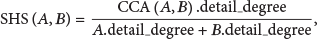
Since each landmark may be associated with an activity, the distance between the predicted and the real activity must be also considered. Due to the fact that such activities are organized in a tree structure (see Figure 4), it is possible to assess the similarity between two activities by means of a conceptual distance. For the current scope, we have used the Semantic-Hierarchical Similarity (SHS) [42] that is defined by the formula

$$\begin{array}{cc}& \mathrm{S}\mathrm{H}\mathrm{S}\left(A,B\right)=\frac{\mathrm{C}\mathrm{C}\mathrm{A}\left(A,B\right)\text{.}\mathrm{d}\mathrm{e}\mathrm{t}\mathrm{a}\mathrm{i}\mathrm{l}\_\mathrm{d}\mathrm{e}\mathrm{g}\mathrm{r}\mathrm{e}\mathrm{e}}{A\text{.}\mathrm{d}\mathrm{e}\mathrm{t}\mathrm{a}\mathrm{i}\mathrm{l}\_\mathrm{d}\mathrm{e}\mathrm{g}\mathrm{r}\mathrm{e}\mathrm{e}+B\text{.}\mathrm{d}\mathrm{e}\mathrm{t}\mathrm{a}\mathrm{i}\mathrm{l}\_\mathrm{d}\mathrm{e}\mathrm{g}\mathrm{r}\mathrm{e}\mathrm{e}},\end{array}$$

(3)

where CCA stands for Closest Common Ancestor, that is, the taxonomy element which is the closest common father of the two elements to be compared. For instance, according to Figure 4, the CCA of the elements care of others and shopping is activities within community.

On the whole, PE is calculated by the following formula:

$$\begin{array}{cc}& \mathrm{P}\mathrm{E}=w_1\times \left(1-\frac{\mathrm{d}\mathrm{i}\mathrm{s}\mathrm{t}\left(\zeta \left(l_{next}^{pred}\right),\zeta \left(l_{next}^{real}\right)\right)}{\mathrm{d}\mathrm{i}\mathrm{s}{\mathrm{t}}_{\mathrm{m}\mathrm{a}\mathrm{x}}}\right)+w_2\times \mathrm{S}\mathrm{H}\mathrm{S}\left(l.a_{next}^{pred},l.a_{next}^{real}\right),\end{array}$$

(4)

where $l_{next}^{pred}$ and $l.a_{next}^{pred}$ are the predictor outcome, $l_{next}^{real}$ and $l.a_{next}^{real}$ are the actual next landmark and its associated activity of the ongoing route, dist is the Euclidean distance, and $\mathrm{d}\mathrm{i}\mathrm{s}{\mathrm{t}}_{\mathrm{m}\mathrm{a}\mathrm{x}}$ is the maximum distance between two points in the dataset's spatial region. Due to the fact that this region takes the form of a circle with radius that equals 12 km in MU and 24 in MA, $\mathrm{d}\mathrm{i}\mathrm{s}{\mathrm{t}}_{\mathrm{m}\mathrm{a}\mathrm{x}}$ was set to 24 km for the former and 48 km for the latter. For the present set of experiments, the weight exponents have been set as $w_{\mathrm{1}}$ = 0.5 and $w_{\mathrm{2}}$ = 0.5.

It is important to remark that, by means of this definition, PE ranges from 0 (when the predicted landmark is completely different to the real one in terms of spatial location and associate activity) to 1 (when there is a perfect match between the real and the predicted landmark). Finally, if the system provided more than one $l_{next}^{pred}$ the PE is calculated as the average one among all the predicted landmarks and the actual one.

4.2. Dataset Preliminary Analysis

Before getting deep into the evaluation of the proposal, we extracted some interesting features of both datasets. In that sense, Figure 12 shows the probability distribution of spatial distance and time intervals between consecutive tweets of the same user.

Figure 12

Complementary Cumulative Distribution Function (CCDF) of spatial distance and time elapsed between consecutive tweets.

From this figure we can see that, in terms of spatial distance between consecutive tweets (Figures 12(a) and 12(b)), short distances are more likely to appear (50% of the tweets in MU and MA are separated by less than 100 m). Nonetheless, longer distances are still likely. Regarding the distribution of time intervals (Figures 12(c) and 12(d)), very long intervals are less likely than shorter ones (50% of the tweets in MU and MA are separated by more than 24 hours). Therefore, we appreciated certain laziness of the Twitter users as they tend to tweet not very frequently and usually not in very different places.

4.3. Effect of Landmark Size

One of the factors that affects most the system performance is the spatial size of the landmarks. This size is mainly defined by the Eps and MinPoints parameters of the landmark discovery algorithm. Figure 13 depicts the PR and PE of the proposal for different Eps × MinPoints configurations for $\{\mathrm{p}\mathrm{e}\mathrm{r}\mathrm{s}\mathrm{o}\mathrm{n}\mathrm{a}\mathrm{l},\mathrm{c}\mathrm{o}\mathrm{l}\mathrm{l}\mathrm{e}\mathrm{c}\mathrm{t}\mathrm{i}\mathrm{v}\mathrm{e}\}$ landmarks. These two parameters indicate the spatial size and the minimum density of points of a landmark. More in detail, we evaluated 4 different configurations, namely, $\{50\times \mathrm{2,100}\times 5\}$ , $\{150\times \mathrm{4,300}\times 8\}$ , $\{250\times \mathrm{8,500}\times 16\}$ , and $\{350\times \mathrm{16,700}\times 32\}$ , where Eps is given in meters.

Figure 13

PR and PE of the system with different configurations of Eps × MinPoints.

As we can see, the size and density of the landmarks are correlated with the PE and PR in both datasets. Regarding the decrease of PR, it has to do with the minimum density required for the landmarks. As it was put forward in Section 3.4.3, LDA does not return any landmark until it receives at least MinPoints of close tweets locations. Consequently, if we increment this factor, the system will have more locations without any assigned landmark (the ones received before getting MinPoints to conform a landmark) which, as a result, decreases the overall PR of the system.

As far as PE is concerned, its decrement trend is related to the spatial dimension of the landmarks. If we increase Eps, which defines the initial radius of a landmark, then the spatial region covered by each landmark will be larger. Hence, in case the system wrongly predicts the next landmark of a user then the distance of this predicted landmark's middle point and the real one will become larger if both elements cover wide spatial regions.

Consequently, given the stated results, we selected the configuration $\{50\times \mathrm{2,100}\times 5\}$ for the remaining evaluation. Figure 14 shows the the collective landmarks generated by the system with these parameters. In that sense, we can see that the higher concentration of collective landmarks actually corresponds to spatial areas with high density of human movement like the city centers. On the contrary, the personal landmarks are more spread across the whole region under study in each city.

Figure 14

Collective and personal landmarks for the selected Eps × MinPoints configuration.

4.4. Memory Saving Evaluation

One of the most improvements of the present work regarding the original LDA is the new mechanism that avoids keeping in memory all the locations collected so far. To give insight into the actual memory saving that we can achieve, Figure 15 shows the overall number of points the system kept in memory to generate the personal landmarks. The number of stored locations is shown with respect to the sheer number of received locations as the system proceeds.

Figure 15

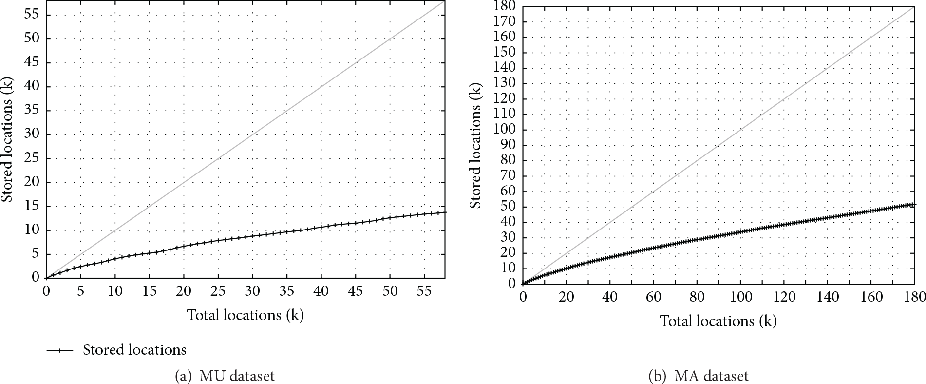
Total number of locations actually stored by the client sides of the proposal. The grey line depicts the imaginary progression of stored locations without the memory saving mechanism.

According to these results, we reduced the number of points in memory up to 75% in both scenarios. Recall that these landmarks are composed in the client side running in the users' contrivances. Thus, this saving is of great utility to enable density-based clustering techniques in memory-constrained scenarios.

4.5. System Performance Evolution

One of the key features of the system is its ability to compose mobility models and make predictions over them on the fly. However, one drawback of this approach is that the system will need a certain convergence period so as to compose a preliminary model rich enough to provide the first predictions. Figure 16 shows the PR and PE as the system processed the dataset. In order to come up with a more reliable test, we have evaluated the system with 5 different subsets each one comprising a slide of the original dataset with 70% of its tweets.

Figure 16

Evolution of the PR and PE of the system.

From this figure, we can appreciate that the PE remained more or less flat with no significant variance throughout all the experiment in both datasets. This way, when only 10% of the dataset was processed our proposal was capable of achieving around 0.85 PE. The reason for this quite high PE even when only a small piece of the dataset has been processed is the spatial distribution of the tweets. As we pointed out in Section 4.2, users tend to post tweets located relatively close among them. This limits the number of total locations that should be considered by the system and, thus, it is more likely to correctly predict the next location of a user. For the sake of clarity, Figure 17 shows the distribution of users with respect to their number of landmarks. In both datasets, the vast majority of users only have one or two different places. This facilitates the achievement of high PE.

Figure 17

Probability distribution of the number of landmarks per user in both datasets.

Concerning the PR, it follows a quite different trend in MA and MU. In the former, the PR remained stable around 13% when the system processed 20% of the dataset. However, in MU, this measurement remarkably varied during the whole experiment. These variations are due to the graph hierarchies generated in the two scenarios. In this frame, MA has much more active users than in MU. Hence, the system is able to generate a complete set of collective landmarks. Since this type of landmark provides support when it is not possible to assign a personal one and, thus, provide a prediction, the generation of a dense network of collective landmarks is a key factor for PR. Figure 18 depicts the evolution of number of collective and personal landmarks along with the sheer number of edges in the personal graphs ${\mathcal{G}}_p$ . As we can see, in MA there were much more collective landmarks compared with personal ones than in MU. This caused that the system in MA was less sensitive to the arrival of new users or locations in terms of PE than in MU.

Figure 18

Evolution of the number of personal and collective landmarks along with the number of edges in the personal graphs.

4.6. Comparison with Alternative Subapproaches

This section is devoted to comparing the present proposal with some of its slight variations so as to uncover which aspects are actually relevant so as to predict future locations and activities with social media data. For that goal, four potential alternatives of the original (O) approach have been considered; namely,

• (i)

no-activity (NA) approach stands for a predictor that does not take into account the current activity of the topic. Therefore, the nodes in the personal and collective graphs only comprise spatial information. The hierarchy of graphs remains the same as in the original approach,

(ii)

no-collective (NC) approach does not have any graph hierarchy, so only the personal graph hierarchy $\mathcal{H}{\mathcal{G}}_p$ is composed and used for prediction,

(iii)

no-activity-no-collective (NANC) approach does not take into account the activity to compose the graphs and make predictions. Moreover, only the personal graph hierarchy $\mathcal{H}{\mathcal{G}}_p$ is composed and used for prediction,

(iv)

no-time-hierarchy (NTH) approach differs from the original approach in the graph hierarchy. In this case, there is neither ${\mathcal{G}}^{workingday}$ nor ${\mathcal{G}}^{weekday}$ in the collective and personal hierarchies. Thus, they only comprise the general personal and collective graphs, ${\mathcal{G}}_p$ and ${\mathcal{G}}_c$ .

Table 4 summarizes the key features of each subsolution. While the no-collective versions (NC, NANC) could be suitable for those deployments where the frequent connection between personal mobile devices and a central server is not desired, the no-activity ones (NA, NANC) could be a proper solution for domains where only spatiotemporal knowledge should be mined.

Table 4

Alternative subapproaches summary.

Approach	Activity	Time	Crowd-sensing
Original (O)	✓	✓	✓
No-activity (NA)		✓	✓
No-collective (NC)	✓	✓
No-activity-no-collective (NANC)		✓
No-time-hierarchy (NTH)	✓		✓

Figure 19 depicts the prediction accuracy of the present proposal (original) and the aforementioned alternatives. Since some of them do not infer the activity, the PE in this figure only considers the spatial distance factor and not the SHS. Hence, a uniform evaluation is performed.

Figure 19

Comparison between the original approach and different variants.

From the aforementioned figure we can draw interesting conclusions. To start with, the most noticeable one is that we observe similar results in both datasets. Therefore, the temporal and spatial size of the dataset under consideration do not really affect the behaviour of each alternative.

Focusing on each of these alternatives, we can see that relying on a collective graph hierarchy $\mathcal{H}{\mathcal{G}}_c$ allows one to greatly improve the performance of the system. This is proved by the fact that the two subapproaches that obtain the worst results are NC and NANC. The reason for the importance of the crowd-sensed mobility model is the nature of the tweet data. For a particular user, his tweets could not be sufficient to compose a mobility model detailed enough. In that case, the usage of the models generated by aggregating data from multiple users turns out to be paramount for route prediction.

Secondly, discarding the activity as parameter to provide predictions increases the PR but inevitably also decreases the accuracy of the predictions. In that sense, the extra level of indexation that the activity provides in the mobility model allows one to meaningfully refine the prediction.

Lastly, according to Figure 19, the time-based graphs allows one to slightly increase the accuracy of the system with respect to the subapproach NTH. Like the activity, considering the time factor adds a new level of indexation in order to select the appropriate path within a graph for making a prediction. As a result, such selection is done in a more accurate manner.

4.7. Mobility Graphs Example

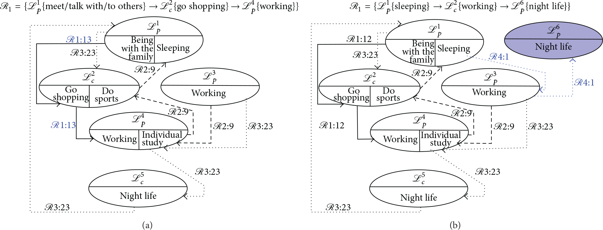
In this section, an actual personal mobility graph ${\mathcal{G}}_p$ made up by the system is described as an illustrative example of the outcome of the proposal.

4.7.1. User #1

Figure 20 shows ${\mathcal{G}}_p$ of one of the users within the MU dataset. As we can see, the system detected 4 different landmarks, 3 of them labelled with different activities.

Figure 20

Personal mobility graph of User #1 in MU.

For the sake of completeness, Figure 21 locates each landmark in a map. In that sense, ${\mathcal{L}}_p^{\mathrm{1}}$ covers a residential area at the outskirts of Murcia city. This is consistent with the home-related activities such landmark is tagged with. Concerning ${\mathcal{L}}_p^{\mathrm{2}}$ , it also comprises a high-school in its spatial area which is also consistent with the study activity. Finally, ${\mathcal{L}}_p^{\mathrm{4}}$ is enclosed in one of the most important parks of the city where usually many outdoor and night activities are organized. Therefore, the labelling of the landmark is also consistent with its location.

Figure 21

Map of landmarks of User #1 in MU.

Moreover, four types of routes of the user were uncovered ${\mathcal{R}}_p^{\mathrm{1}}=\{{\mathcal{L}}_p^{\mathrm{1}}\{eating\}$ → ${\mathcal{L}}_p^{\mathrm{3}}$ → ${\mathcal{L}}_p^{\mathrm{4}}\{drinking\}\}$ , ${\mathcal{R}}_p^{\mathrm{2}}=\{{\mathcal{L}}_p^{\mathrm{1}}\{talk/meet\hspace{0.17em}\hspace{0.17em}to/with\hspace{0.17em}\hspace{0.17em}others\}$ → ${\mathcal{L}}_p^{\mathrm{3}}$ → ${\mathcal{L}}_p^{\mathrm{4}}\{talk/meet\hspace{0.17em}\hspace{0.17em}to/with\hspace{0.17em}\hspace{0.17em}others\}\}$ , ${\mathcal{R}}_p^{\mathrm{3}}=\{{\mathcal{L}}_p^{\mathrm{1}}\{individual\hspace{0.17em}\hspace{0.17em}study\}$ → ${\mathcal{L}}_p^{\mathrm{2}}\{academic\hspace{0.17em}\hspace{0.17em}activities\}\}$ , and ${\mathcal{R}}_p^{\mathrm{4}}=\{{\mathcal{L}}_p^{\mathrm{1}}\{resting\}$ → ${\mathcal{L}}_p^{\mathrm{2}}\{academic\hspace{0.17em}\hspace{0.17em}activities\}\}$ . Bearing in mind the location and labelling of each landmark, we could infer that the first two routes stand for mobility routes related to the user's free time and the third one has to do with a routine linked to his professional/student occupation.

4.7.2. User #2

This user has been extracted from the MA dataset. The system was able to recognize three different personal landmarks according to his graph in Figure 22. Again, we can intuitively infer that ${\mathcal{L}}_p^{\mathrm{1}}$ represents the home of the user according to its associated topics, whereas the other two are more related to academic and leisure activities. In addition to that, four different routes were extracted by the system, ${\mathcal{R}}_p^{\mathrm{1}}=\{{\mathcal{L}}_p^{\mathrm{1}}\{get\hspace{0.17em}\hspace{0.17em}in/out\hspace{0.17em}\hspace{0.17em}bed\}\to {\mathcal{L}}_p^{\mathrm{1}}\to {\mathcal{L}}_p^{\mathrm{2}}\}$ , ${\mathcal{R}}_p^{\mathrm{2}}=\{{\mathcal{L}}_p^{\mathrm{2}}\{academic\hspace{0.17em}\hspace{0.17em}activities\}\to {\mathcal{L}}_p^{\mathrm{1}}\{resting\}\}$ , ${\mathcal{R}}_p^{\mathrm{3}}=\{{\mathcal{L}}_p^{\mathrm{1}}\{talk/meet\hspace{0.17em}\hspace{0.17em}to/with\hspace{0.17em}\hspace{0.17em}others\}\to {\mathcal{L}}_p^{\mathrm{3}}\{eating\}\}$ , and ${\mathcal{R}}_p^{\mathrm{4}}=\{{\mathcal{L}}_p^{\mathrm{3}}\{go\hspace{0.17em}\hspace{0.17em}clubbing\}\to {\mathcal{L}}_p^{\mathrm{1}}\{sleeping\}\}$ .

Figure 22

Personal mobility graph of User #2 in MA.

Finally, Figure 23 shows the location of the three landmarks in Madrid city.

Figure 23

Map of landmarks of User #2 in MA.

Figure 24

Basic activities taxonomy.

Figure 25

Activities within community taxonomy.

All in all, both users have one landmark with higher number of activity tags compared to the others. This landmark can be usually mapped to the user's home. In addition to that, landmarks representing the user's office/school and his favourite/most visited leisure place have been also uncovered. The discovery of these three types of regions makes sense as they are probably the places where a person spends more time and, thus, writes most of his tweets.

4.8. Results Discussion

On the whole, the present evaluation has allowed coming up with several interesting conclusions about the proposal and Twitter itself as mobility data-source:

• (i)

Firstly, an analysis of datasets of two different cities shows that half of Twitter users tend to write no more than one tweet per day and in very close locations. Therefore, they seem rather reluctant to write several tweets in many different locations.

(ii)

The spatial size configuration for the landmark should be carefully selected beforehand as this parameter meaningfully affects the system performance. According to the results for the two datasets under evaluation, it is more suitable to define small landmarks with low density of points given the aforementioned laziness of users.

(iii)

The modification of the density-based clustering to avoid keeping in memory all the processed locations achieves savings of more than 75% in terms of stored locations. This can be a suitable approach to execute this type of clustering in memory-constrained scenarios.

(iv)

Results confirm that the PR of the system is closely related to the level of detail of the graph hierarchy. In that sense, the generation of collective landmarks has proved to be an interesting approach to keep in acceptable terms the PR.

(v)

Finally, the devised hierarchy of mobility graphs comprising personal and crowd-sensed knowledge allows combining both types of information in a suitable way. In particular, the collective hierarchy $\mathcal{H}{\mathcal{G}}_p$ turns out to be paramount for a correct prediction outcome.

5. Conclusion

The endless improvement of built-in positioning sensors in personal mobile devices and the pervasiveness of social media data allows capturing an unprecedented amount of location data that is not constrained to the spatiotemporal dimension but also enlarged with semantic meaning.

The present work intends to be one of the first steps towards the full usage of both the spatiotemporal and semantic aspects of the aforementioned type of data. In particular, given the geotagged tweets within an area of interest, the devised solution is able to extract the mobility flows at different levels of detail by means of a crowd-sensing approach. In order to orchestrate the different components of the proposal, the Complex Event Processing (CEP) approach has been applied. Moreover, a complete evaluation of different features of the solution with two real-world datasets has been described.

To conclude, further work will focus on coming up with automatic detection of similarities among groups of users in terms of mobility and activity. This will generate intermediate mobility graphs, related to specific groups of users, allocated between the personal and the collective ones. This would enrich even more the proposed graph hierarchy.