Node-Gosper Curve-Based Unknown Sensor Localization Using Single Mobile Anchor in Wireless Sensor Networks

Abstract

The node-Gosper curve is a fractal space-filling curve constructed by recursively replacing each node by a seven-segment generator curve. Here, we propose a novel scheme for describing the path of a node-Gosper curve; the scheme can be used to calculate the coordinates of each turning point of the curve efficiently. The node-Gosper curve serves as a routing path for a single mobile anchor to help unknown sensors locate themselves in the wireless sensor network. In our proposed localization method, the mobile anchor travels along the node-Gosper curve, which covers the entire sensing field, and when it reaches the turning points of the node-Gosper curve, it broadcasts its current location to unknown sensors within a preset communication range. Each unknown sensor estimates its location when it receives at least three messages from the mobile anchor from different locations. Experimental results show that the proposed method outperforms several well-known mobile anchor localization methods in terms of localization accuracy and energy consumption.

1. Introduction

A wireless sensor network (WSN) consists of spatially distributed autonomous sensors that cooperatively monitor a deployed region for physical or environmental conditions, such as temperature, sound, vibration, pressure, motion, and pollutants. Sensor nodes are usually powered by batteries, and they have limited storage capacity and on-board processing and radio capabilities. Minimizing the energy consumption of sensor nodes and maximizing the network lifetime are crucial in the design of WSN routing protocols.

Many WSN applications require knowledge of the accurate location of each sensor. However, in certain hazardous environments, it is difficult to measure the positions of sensors manually. Fortunately, localization techniques for estimating the locations of sensors exist. Perhaps the most popular localization approach is to install a Global Positioning System (GPS) module on the sensors. Despite the decreasing cost of GPS receivers, it remains too costly and energy inefficient for large-scale installation in a WSN. Therefore, other techniques should be developed for solving localization problems in WSNs.

Because of advancements in mobile robot technology in recent years, it is feasible to use mobile robots, which have the capability to determine their own positions and to receive/transmit messages from/to other sensors in a WSN, as mobile anchors, and equip them with wireless sensors. Therefore, for a WSN, we can use such mobile anchors to travel along a predetermined path and broadcast their locations at each stop to unknown sensors (sensors whose positions are unknown) to help them locate themselves by using localization algorithms.

A Gosper curve [1] is a space-filling curve constructed by recursively replacing each line segment by a seven-segment generator curve. The space filled by the curve is called Gosper island. Figure 1(a) shows the first level of a Gosper curve along with the corresponding Gosper island. Suppose that we intend using the Gosper curve as the routing path for a mobile anchor for gathering or disseminating data and we consider the regions enclosed by regular hexagons as the basic regions for grouping sensors in a WSN; a routing path passing through the centers of the basic hexagons would be much more useful than a routing path passing through the chords of the hexagons (such as a Gosper curve). The special type of Gosper curve that passes through the centers of hexagons is called node-Gosper curve [2], and it is constructed by replacing each node by a seven-segment generator curve. The space filled by the node-Gosper curve is called node-Gosper island, and it is identical to the traditional Gosper island.

Figure 1

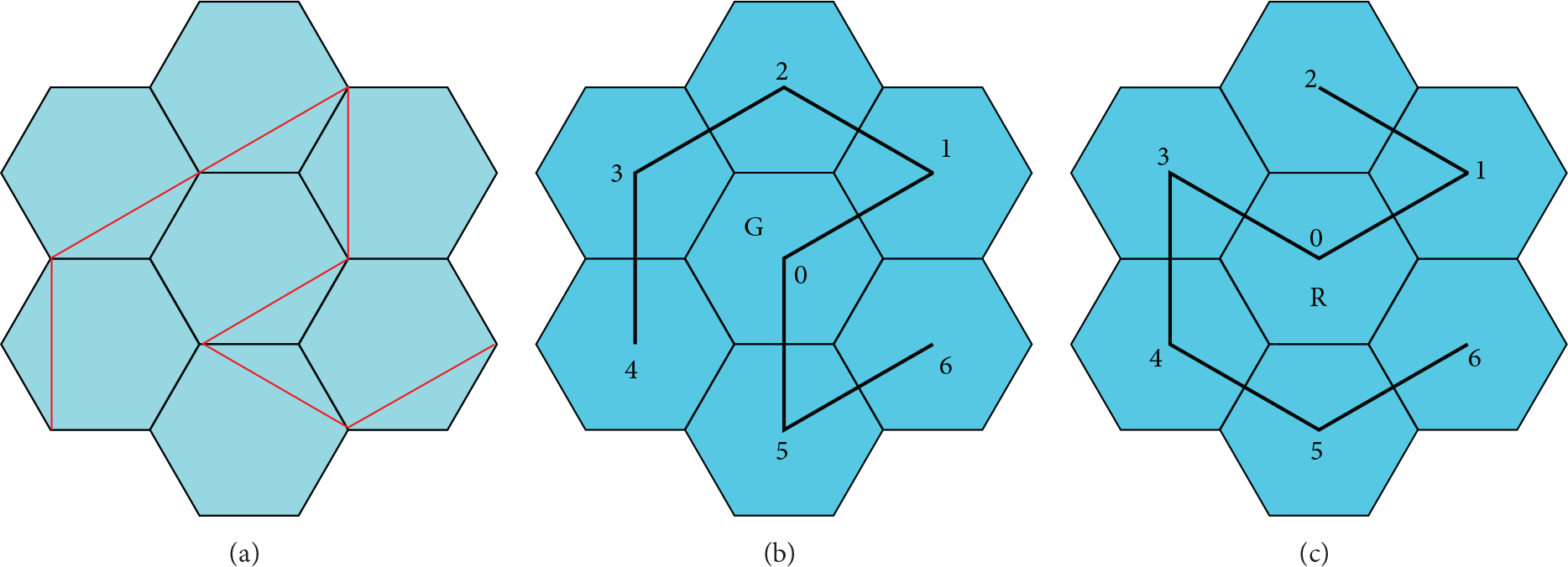
Level-1 Gosper curve and node-Gosper curves with their corresponding Gosper islands. (a) Gosper curve; (b) type-G node-Gosper curve; (c) type-R node-Gosper curve.

There are two types of node-Gosper generator curves: type-G and type-R. Node-Gosper generator curves are level-1 node-Gosper curves. Figures 1(b) and 1(c) show the two types of level-1 node-Gosper curves along with the corresponding Gosper islands. Seven copies of a Gosper island can be joined together to obtain a form that has a shape similar to the shape of the original Gosper island. The resulting form is scaled up by a factor of $\sqrt{7}$ in each dimension [2]. Figure 2 shows the level-2 and level-3 Gosper islands and the corresponding node-Gosper curves.

Figure 2

(a) Level-2 Gosper island (including its corresponding type-R node-Gosper curve) and (b) level-3 Gosper island (including its corresponding type-R node-Gosper curve).

An L-system (or Lindenmayer system) [2] is a recursive string-rewriting system that is used to model many self-similar fractal geometries. In general, we can use the following production rules of the L-system to generate node-Gosper curves:

• (1)

G $\leftarrow$ G $rr\uparrow l$ R $rr\uparrow l$ R $r\uparrow ll$ G $r\uparrow ll$ G $rr\uparrow l$ G $r\uparrow ll$ R $\hspace{0.17em}\hspace{0.17em}\mid \hspace{0.17em}\hspace{0.17em}\uparrow rr\uparrow r\uparrow ll\uparrow l\uparrow l\uparrow$

(2)

R $\leftarrow$ G $rr\uparrow l$ R $r\uparrow ll$ R $rr\uparrow l$ R $rr\uparrow l$ G $r\uparrow ll$ G $r\uparrow ll$ R $\hspace{0.17em}\hspace{0.17em}\mid \hspace{0.17em}\hspace{0.17em}\uparrow r\uparrow r\uparrow rr\uparrow l\uparrow ll\uparrow$

where G and R are nonterminals representing type-G and type-R node-Gosper curves, respectively, and l and r represent clockwise and counterclockwise rotations by 60°, respectively; $\uparrow$ represents forward motion by unit distance.

It is very convenient to use the L-system to describe the node-Gosper curve. However, the L-system cannot be used to calculate the position of a node on the path without calculating the positions of all its predecessor nodes. In this study, we determined several geometric properties of the node-Gosper curves and exploited these properties to develop a new addressing scheme for the Gosper islands. We derived a new method to describe the path of the node-Gosper curve on the basis of the new addressing scheme. The description can be used to efficiently calculate the coordinates of any turning point on the path.

In our proposed localization method, the node-Gosper curve is used as the routing path; the mobile anchor traverses this path and broadcasts its position at each turning point to the unknown sensors within its communication range to help them locate themselves.

2. Related Work

Recently, many researches have been presented on the use of mobile anchors for locating unknown sensors in a WSN. Most of them have used straight lines, triangles, or squares as the basis for constructing routing paths [7–10]. Only three regular geometric shapes, namely, triangle, square, and hexagon, can be used to tessellate a two-dimensional plane. For a given circle circumscribing each basic regular shape, the number of hexagons required to tessellate the plane is lesser than the number of triangles or squares [11]. In this study, we consider using hexagons as the basis for constructing the routing paths for localization in a WSN.

Koutsonikolas et al. [7] proposed two simple path planning schemes, namely, SCAN and DOUBLE SCAN, for the mobile anchor node; these schemes were part of the localization scheme used by them. In SCAN, the mobile anchor node travels along a single dimension (e.g., along the x-axis or y-axis), and the distance between two adjacent segments of the node trajectory defines the resolution of the trajectory. SCAN is simple and provides uniform coverage to the entire network, as shown in Figure 3(a). However, the collinearity of the beacons degrades the accuracy of the localization results. In DOUBLE SCAN, the collinearity problem is overcome by driving the anchor in both the x-axis and the y-axis directions, as shown in Figure 3(b). However, although this strategy improves the localization performance of the sensor nodes, the path length is doubled compared with that of SCAN, and, therefore, the energy overhead increases.

Figure 3

Routing paths in SCAN and DOUBLE SCAN.

In [8], the authors proposed a mobile anchor localization method, called triangle grid scan (TGS), based on the triangular tessellation of a plane. In TGS, the entire network is divided into many nonoverlapping triangular cells. A mobile anchor traverses the path in a snake-like manner, as shown in Figure 4(a), and broadcasts location messages from each vertex to the unknown sensors within the communication range.

Figure 4

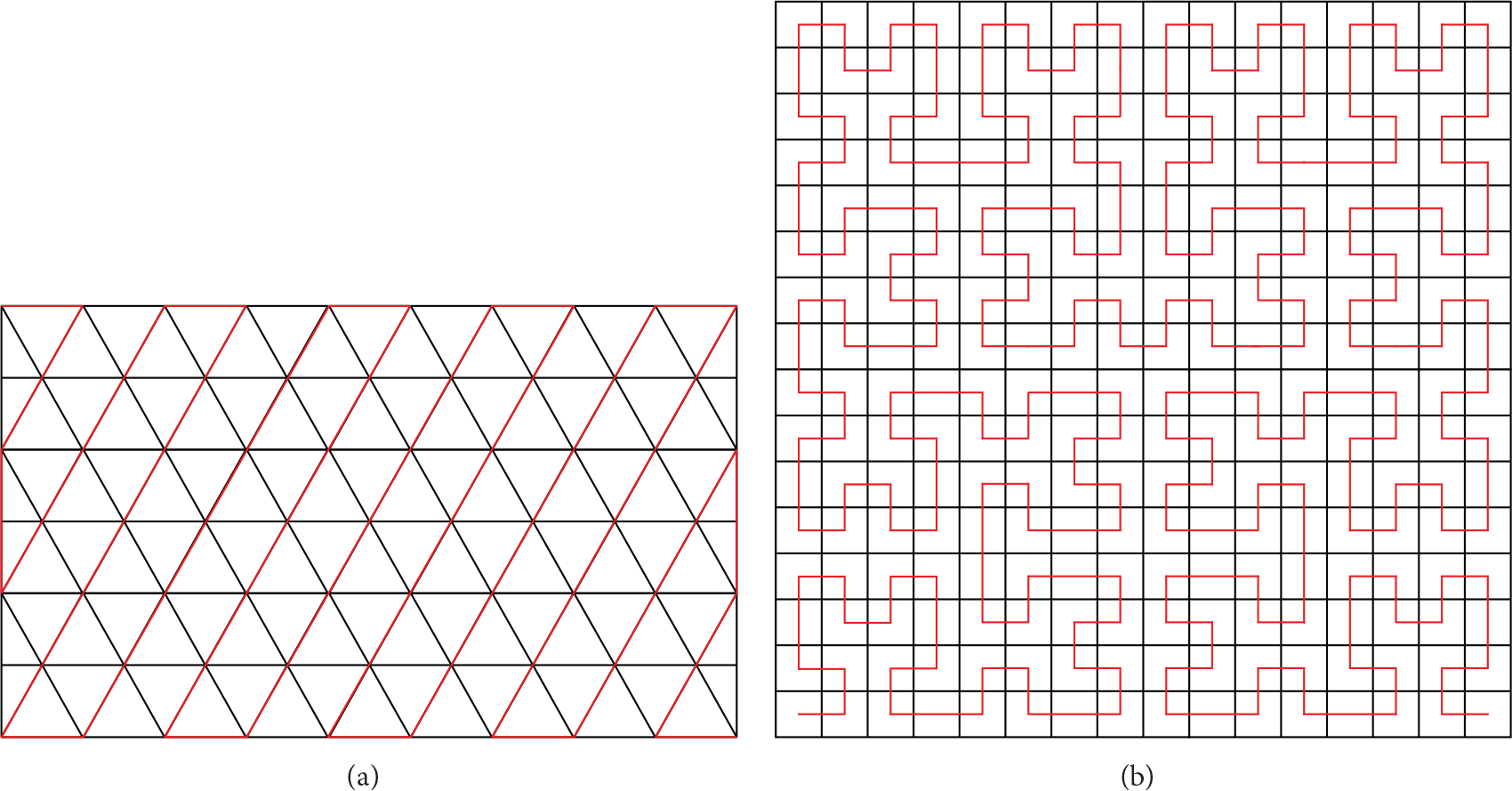
(a) Routing path in TGS and (b) fourth-order Hilbert curve in a square-tessellated plane.

In the studies reported in [9, 10], Hilbert curves served as the routing paths for the mobile anchor used for localizing unknown sensors in a WSN. The Hilbert curve is a space-filling curve that passes through the center of every square of a square grid in a plane. The basic Hilbert curve on a 2 × 2 grid is a U-shaped curve passing through the center of each square quadrant. To derive a curve of order i from a basic curve, each vertex of the basic curve is replaced by a curve of order $i-1$ , which may be appropriately rotated or flipped. Figure 4(b) shows a Hilbert curve of order four. The mobile anchor travels along the Hilbert curve and broadcasts its location at each turning point (called h-key) of the curve. Each unknown sensor receives a set of location packets from the mobile anchor, and the sensor then calculates its position through trigonometric relations from the positions of the neighboring h-keys and the estimated distances between the unknown sensor and the h-keys.

In this study, we used a node-Gosper curve, which is based on the hexagonal tessellation of a plane, as the routing path for mobile anchor localization. In Table 1, the total routing path length and the number of mobile anchor broadcasts under the same radius of circumscribed circle ( $r=10$  m) for each unit regular shape are compared for localization methods that use TGS, Hilbert, and node-Gosper curves as routing paths.

Table 1

Number of radio broadcasts and total routing path length required in the localization methods based on TGS, Hilbert, and node-Gosper curves.

Routing method ${}^{\ast }$	Sensing area (km2)	Number of radio broadcasts	Path length (m)	Number of radio broadcasts per km2 (times/km2)	Path length per km2 (m/km2)
TGS ( $\mathit{9}\times \mathit{6}$ triangles) Figure 4(a).	14.030	67	1168	4.8	83.3
Hilbert (order 4) Figure 4(b).	51.200	256	3606	5.0	70.4
Node-Gosper (level 3) Figure 2(b).	89.115	343	5923	3.8	66.5

${}^{\ast }$ Radius of the circumscribed circle of each basic regular polygon $r=\mathit{10}$  m.

Clearly, for the same normalized area (1000 m² or km²), the node-Gosper curve involves a lesser number of radio broadcasts compared with TGS and the Hilbert curve; moreover, the path length of the node-Gosper curve is shorter than those of the other two curves, implying that the use of the node-Gosper curve as the routing path for mobile anchor localization leads to less energy consumption and a shorter routing time compared with the use of the other two methods. This observation inspired further investigation into the localization method based on a node-Gosper curve.

3. Properties of Node-Gosper Curves and the Proposed Localization Method

Since a node-Gosper curve passes through the centers of hexagons in its corresponding Gosper island, in this section, we first introduce two addressing schemes related to the hexagons in a hexagonally tessellated plane. We then exploited several properties of these two addressing schemes and applied them to calculate the Cartesian coordinates of the center points of hexagons in the Gosper island. The localization method in which a node-Gosper curve is used as the routing path is presented at the end of this section.

3.1. Two Addressing Schemes for a Hexagonally Tessellated Plane

Tessellation is the process of covering a two-dimensional plane by repeating a geometric shape, without any overlap or gap. Regular tessellation refers to tessellation in which a two-dimensional plane is covered with regular polygons of the same shape and size.

There are several approaches for addressing a hexagon in a hexagonally tessellated plane (for details, the reader is referred to [12]). In this study, we used an addressing scheme based on the polar system, called ring-based addressing scheme, to index each hexagon in a plane. Here, we show how the polar system and linear combinations of vectors can be used to directly transform ring-based addresses of hexagons to their corresponding Cartesian coordinates. The authors in [13] used a similar approach to index the hexagons in a hexagonally tessellated plane; they called it honeycomb architecture and used the index system to disseminate data.

In the ring-based addressing scheme, the plane tessellated by regular hexagons is considered to comprise concentric hexagonal rings centered at the center of the plane, as shown in Figure 5(a). Suppose that the center of the plane is at the origin $(\mathrm{0,0})$ and that the plane is tessellated with regular hexagons of length r. For simplicity, we assume $r=1$ in the following discussion.

Figure 5

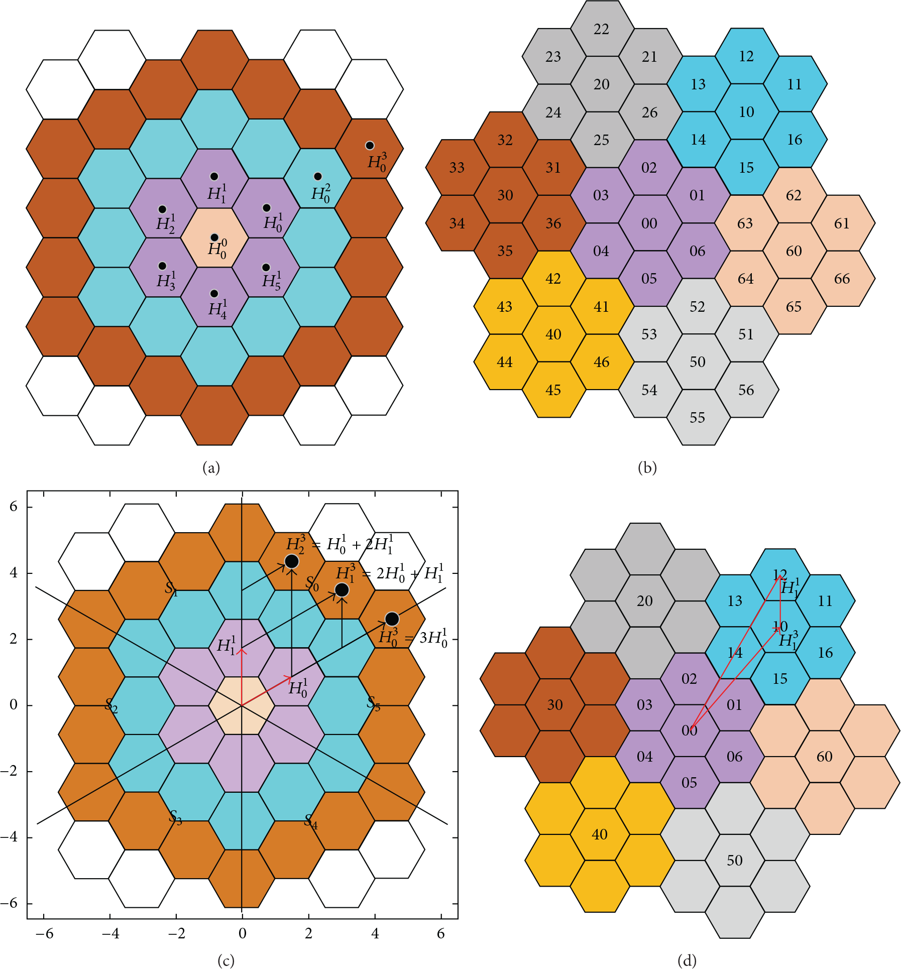
(a) Ring-based addressing scheme for hexagons in a hexagonally tessellated plane. (b) Addresses of the level-2 Gosper island according to the base-7 addressing scheme. (c) The six sectors of the hexagonally tessellated plane and the linear combinations for $H_0^{\mathrm{3}}$ , $H_1^3$ , and $H_2^3$ . (d) Cartesian coordinate calculation for the center of the hexagon with address 12.

Let the center of the central hexagon be denoted by $H_0^0$ . Thus, $H_0^0=(\mathrm{0,0})$ . The hexagons immediately surrounding the central hexagon constitute the first hexagonal ring. Similarly, the hexagons immediately surrounding the $(n-1)\mathrm{t}\mathrm{h}$ hexagonal ring constitute the $n\mathrm{t}\mathrm{h}$ hexagonal ring. The center of the $k\mathrm{t}\mathrm{h}$ hexagon in the $n\mathrm{t}\mathrm{h}$ hexagonal ring is denoted as $H_k^n$ . Figure 5(a) shows the notation used for hexagon centers in the first hexagonal ring. There are six hexagons in the first hexagonal ring, and their centers in Cartesian coordinates can be calculated from their polar coordinates as follows:

$$\begin{array}{cc}& H_i^{\mathrm{1}}=\sqrt{\mathrm{3}}\left(\cos \left(\frac{\pi }{\mathrm{6}}+\frac{i\times \pi }{\mathrm{3}}\right),\sin \left(\frac{\pi }{\mathrm{6}}+\frac{i\times \pi }{\mathrm{3}}\right)\right),\hspace{1em}\mathrm{w}\mathrm{h}\mathrm{e}\mathrm{r}\mathrm{e}\hspace{0.17em}\hspace{0.17em}i=\mathrm{0,1},\dots ,\mathrm{5}.\end{array}$$

(1)

Therefore,

$$\begin{array}{cc}& H_{\mathrm{0}}^{\mathrm{1}}=\left(\frac{\mathrm{3}}{\mathrm{2}},\frac{\sqrt{\mathrm{3}}}{\mathrm{2}}\right),\\ H_{\mathrm{1}}^{\mathrm{1}}=\left(\mathrm{0},\sqrt{\mathrm{3}}\right),\\ H_{\mathrm{2}}^{\mathrm{1}}=\left(-\frac{\mathrm{3}}{\mathrm{2}},\frac{\sqrt{\mathrm{3}}}{\mathrm{2}}\right),\\ H_{\mathrm{3}}^{\mathrm{1}}=\left(-\frac{\mathrm{3}}{\mathrm{2}},-\frac{\sqrt{\mathrm{3}}}{\mathrm{2}}\right),\\ H_{\mathrm{4}}^{\mathrm{1}}=\left(\mathrm{0},-\frac{\sqrt{\mathrm{3}}}{\mathrm{2}}\right),\\ H_{\mathrm{5}}^{\mathrm{1}}=\left(\frac{\mathrm{3}}{\mathrm{2}},-\frac{\sqrt{\mathrm{3}}}{\mathrm{2}}\right).\end{array}$$

(2)

Furthermore, the hexagonally tessellated plane can be divided into six equal-sized sectors $S_0,S_1,\dots ,S_5$ as shown in Figure 5(c). Considering $H_i^1$ to be a vector, sector $S_i$ can be represented as a linear combination of $H_i^1$ and $H_{i+1}^1$ :

$$\begin{array}{cc}& S_i=\left\{\left(x,y\right)\in R^{\mathrm{2}}\mid \left(x,y\right)=a{H}_i^{\mathrm{1}}+b{H}_{i+\mathrm{1}}^{\mathrm{1}},\hspace{0.17em}\hspace{0.17em}\forall a>\mathrm{0},\hspace{0.17em}\hspace{0.17em}b\ge \mathrm{0},\hspace{0.17em}\hspace{0.17em}a,b\in R\right\},\hspace{1em}\mathrm{w}\mathrm{h}\mathrm{e}\mathrm{r}\mathrm{e}\hspace{0.17em}\hspace{0.17em}i=\mathrm{0},\dots ,\mathrm{5},\end{array}$$

(3)

and $H_{\mathrm{6}}^{\mathrm{1}}=H_{\mathrm{0}}^{\mathrm{1}}$ .

In particular, the center of the $k\mathrm{t}\mathrm{h}$ hexagon in the $n\mathrm{t}\mathrm{h}$ hexagonal ring can be represented as the combination of $H_i^1$ and $H_{i+1}^1$ as follows:

$$\begin{array}{cc}& H_k^n=\left(n-\left(k-n\times i\right)\right)H_i^{\mathrm{1}}+\left(k-n\times i\right)H_{i+\mathrm{1}}^{\mathrm{1}},\hspace{1em}\mathrm{w}\mathrm{h}\mathrm{e}\mathrm{r}\mathrm{e}\hspace{0.17em}\hspace{0.17em}i=⌊\frac{k}{n}⌋.\end{array}$$

(4)

For example, $H_{\mathrm{0}}^{\mathrm{3}}=\mathrm{3}{H}_{\mathrm{0}}^{\mathrm{1}}=\mathrm{3}\left[\mathrm{3}/\mathrm{2},\sqrt{\mathrm{3}}/\mathrm{2}\right]=\left[\mathrm{9}/\mathrm{2},\mathrm{3}\sqrt{\mathrm{3}}/\mathrm{2}\right]$ , $H_{\mathrm{1}}^{\mathrm{3}}=\mathrm{2}{H}_{\mathrm{0}}^{\mathrm{1}}+H_{\mathrm{1}}^{\mathrm{1}}=\mathrm{2}\left[\mathrm{3}/\mathrm{2},\sqrt{\mathrm{3}}/\mathrm{2}\right]+\left[\mathrm{0},\sqrt{\mathrm{3}}\right]=[\mathrm{3,2}\sqrt{\mathrm{3}}]$ , and $H_{\mathrm{2}}^{\mathrm{3}}=H_{\mathrm{0}}^{\mathrm{1}}+\mathrm{2}{H}_{\mathrm{1}}^{\mathrm{1}}=\left[\mathrm{3}/\mathrm{2},\sqrt{\mathrm{3}}/\mathrm{2}\right]+\mathrm{2}\left[\mathrm{0},\sqrt{\mathrm{3}}\right]=\left[\mathrm{3}/\mathrm{2},\mathrm{5}\sqrt{\mathrm{3}}/\mathrm{2}\right]$ , as shown in Figure 5(c). Therefore, from (4), we can calculate the Cartesian coordinates of the center of any hexagon in the hexagonally tessellated plane.

In the original document on Gosper islands [14], the author did not provide any addressing method for indexing the hexagons in the Gosper islands. In the current study, we used an addressing method provided in [12], called base-7 addressing scheme, to index the hexagons in the Gosper islands.

In a level-n Gosper island, it is possible to uniquely index every hexagon by using an n-digit base-7 number, where each digit indicates the specific position of a lower-level Gosper island in the superlevel Gosper island, 0 indicates the center hexagon, and numerals 1–6 indicate hexagons counted counterclockwise around the center hexagon. This method of indexing each hexagon in a Gosper island is referred to as the base-7 addressing scheme. Figure 5(b) shows the indexes of hexagons in a level-2 Gosper island.

Unfortunately, directly using the base-7 addressing scheme to calculate the Cartesian coordinates of the center of a given hexagon in the Gosper island is fairly complicated, as described in a previous paper [15]. Therefore, in this study, for the hexagons in the tessellated plane, the ring-based addressing scheme was used to map the base-7 addresses of the hexagons in the Gosper island to the Cartesian coordinates of the centers of the hexagons.

3.2. Converting the Base-7 Address to Cartesian Coordinates for Gosper Islands

Clearly, in Figure 5(b), the centers of the six surrounding level-1 sub-Gosper islands in the level-2 Gosper island are located in the same hexagonal ring—the third hexagonal ring. Moreover, in Figure 6, the centers of the six surrounding sub-Gosper islands in Gosper islands at levels 2–4 are located in the 3rd, 7th, and 21st hexagonal rings, respectively.

Figure 6

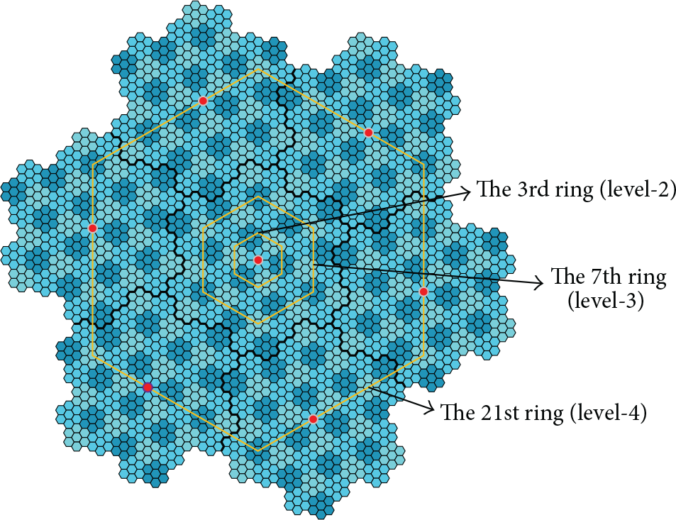
Ranks of hexagonal rings that contain the sub-Gosper island centers in Gosper islands at levels 2, 3, and 4.

In general, the rank (the position in the sequence of the concentric hexagonal rings) of the hexagonal ring in which the centers of the six surrounding sub-Gosper islands are located in a given level of Gosper island can be obtained from the following lemma. The formal proof of Lemma 1 is presented in the Appendix.

Lemma 1.

Given level n, $n\ge 1$ , of a Gosper island, the centers of its six level- $(n-1)$ surrounding sub-Gosper islands are located in the $r(n)$ th hexagonal ring, where

$$\begin{array}{cc}& r\left(n\right)=\left\{\begin{array}{cc}{\mathrm{7}}^{\left(\left(n-\mathrm{1}\right)/\mathrm{2}\right)}\hfill & if\hspace{0.17em}\hspace{0.17em}n\hspace{0.17em}\hspace{0.17em}is\hspace{0.17em}\hspace{0.17em}an\hspace{0.17em}\hspace{0.17em}odd\hspace{0.17em}\hspace{0.17em}number\hfill \\ {\mathrm{7}}^{\left(\left(n-\mathrm{2}\right)/\mathrm{2}\right)}\times \mathrm{3}\hfill & if\hspace{0.17em}\hspace{0.17em}n\hspace{0.17em}\hspace{0.17em}is\hspace{0.17em}\hspace{0.17em}an\hspace{0.17em}\hspace{0.17em}even\hspace{0.17em}\hspace{0.17em}number.\hfill \end{array}\right.\end{array}$$

(5)

For example, in the level-2 Gosper island, the centers of its six surrounding level-1 sub-Gosper islands are located in the $7^{(\left(2-2\right)/2)}\times 3=3\mathrm{r}\mathrm{d}$ hexagonal ring. In the level-3 Gosper island, the centers of its six surrounding level-2 sub-Gosper islands are located in the $7^{(\left(3-1\right)/2)}=7\mathrm{t}\mathrm{h}$ hexagonal ring, and in the level-4 Gosper island, the centers of its six surrounding level-3 sub-Gosper islands are located in the $7^{(\left(4-2\right)/2)}\times 3=21\mathrm{s}\mathrm{t}$ hexagonal ring.

We now show how Lemma 1 can be used to calculate the Cartesian coordinates of the center of any given hexagon in the level-n Gosper island addressed using the base-7 addressing scheme. In the following, for convenience of illustration, we consider the Cartesian coordinates $(x,y)$ of any point in the two-dimensional space as an Euclidean vector $[x,y]$ , if necessary.

Let $d_n{d}_{n-1}\cdots d_2{d}_1$ be the address of hexagon A in the level-n Gosper island. In particular, $d_n$ indicates that A is a hexagon in the $d_n$ th level-( $n-1$ ) sub-Gosper island. Furthermore, $d_{n-1}$ indicates that A is in the ${(d}_{n-1})\mathrm{t}\mathrm{h}$ level-( $n-2$ ) sub-Gosper island in its super-Gosper island of level ( $n-1$ ). In general, $d_{(n-k)}$ indicates that A is in the ${(d}_{n-k})$ th level-( $n-k-1$ ) sub-Gosper island in its super-Gosper island of level $(n-k)$ , where $\mathrm{0}\le k\le n-\mathrm{1}$ . Therefore, by the head-to-tail rule of vector addition, the vector of the center of A can be obtained as a linear combination of the vectors of the n centers from its level- $(n-1)$ sub-Gosper island to its inward level-0 sub-Gosper island.

Let the vector of the center point of hexagon A be denoted by center (A). The vector can be obtained as the following linear combination of vectors:

$$\begin{array}{cc}& \mathrm{C}\mathrm{e}\mathrm{n}\mathrm{t}\mathrm{e}\mathrm{r}\left(A\right)=\left\{\begin{array}{cc}{H}_{\left(d_n-\mathrm{1}\right)\times r\left(n\right)}^{r\left(n\right)}+H_{\left(d_{n-\mathrm{1}}-\mathrm{1}\right)\times r\left(n-\mathrm{1}\right)+r\left(n-\mathrm{2}\right)}^{r\left(n-\mathrm{1}\right)}+\cdots +H_{\left(d_{\mathrm{2}}-\mathrm{1}\right)\times r\left(\mathrm{2}\right)+r\left(\mathrm{1}\right)}^{r\left(\mathrm{2}\right)}+H_{\left(d_{\mathrm{1}}-\mathrm{1}\right)\times r\left(\mathrm{1}\right)}^{r\left(\mathrm{1}\right)},\hfill & \mathrm{i}\mathrm{f}\hspace{0.17em}\hspace{0.17em}n\hspace{0.17em}\hspace{0.17em}\mathrm{i}\mathrm{s}\hspace{0.17em}\hspace{0.17em}\mathrm{a}\mathrm{n}\hspace{0.17em}\hspace{0.17em}\mathrm{o}\mathrm{d}\mathrm{d}\hspace{0.17em}\hspace{0.17em}\mathrm{n}\mathrm{u}\mathrm{m}\mathrm{b}\mathrm{e}\mathrm{r}\hfill \\ H_{\left(d_n-\mathrm{1}\right)\times r\left(n\right)+r\left(n-\mathrm{1}\right)}^{r\left(n\right)}+H_{\left(d_{n-\mathrm{1}}-\mathrm{1}\right)\times r\left(n-\mathrm{1}\right)}^{r\left(n-\mathrm{1}\right)}+\cdots +H_{\left(d_{\mathrm{2}}-\mathrm{1}\right)\times r\left(\mathrm{2}\right)+r\left(\mathrm{1}\right)}^{r\left(\mathrm{2}\right)}+H_{\left(d_{\mathrm{1}}-\mathrm{1}\right)\times r\left(\mathrm{1}\right)}^{r\left(\mathrm{1}\right)},\hfill & \mathrm{i}\mathrm{f}\hspace{0.17em}\hspace{0.17em}n\hspace{0.17em}\hspace{0.17em}\mathrm{i}\mathrm{s}\hspace{0.17em}\hspace{0.17em}\mathrm{a}\mathrm{n}\hspace{0.17em}\hspace{0.17em}\mathrm{e}\mathrm{v}\mathrm{e}\mathrm{n}\hspace{0.17em}\hspace{0.17em}\mathrm{n}\mathrm{u}\mathrm{m}\mathrm{b}\mathrm{e}\mathrm{r}.\hfill \end{array}\right.\end{array}$$

(6)

Here, $H_j^i$ , as in Formula (4), denotes the vector of the center point of the hexagon located at the jth position of the ith ring and $H_j^i=\left[\mathrm{0,0}\right]$ if $j<0$ . $r(k)$ , $k\ge \mathrm{1}$ , is defined in Lemma 1, and $r\left(\mathrm{0}\right)=\mathrm{0}$ . Combining the cases of odd and even numbers, we have

$$\begin{array}{cc}& \mathrm{C}\mathrm{e}\mathrm{n}\mathrm{t}\mathrm{e}\mathrm{r}\left(A\right)={{\displaystyle \sum }}_{i=\mathrm{1}}^n{H}_{\left(d_i-\mathrm{1}\right)\times r\left(i\right)+r\left(i-\mathrm{1}\right)\times \left[\left(i-\mathrm{1}\right)\mathrm{mod}\mathrm{2}\right]}^{r\left(i\right)}.\end{array}$$

(7)

The following theorem summarizes the preceding discussion.

Theorem 2.

Given a hexagon A in the level-n Gosper island with base-7 address $d_n{d}_{n-1}\cdots d_2{d}_1$ ,

$$\begin{array}{cc}& Center\left(A\right)={{\displaystyle \sum }}_{i=\mathrm{1}}^n{H}_{\left(d_i-\mathrm{1}\right)\times r\left(i\right)+r\left(i-\mathrm{1}\right)\times \left[\left(i-\mathrm{1}\right)\mathrm{mod}\mathrm{2}\right]}^{r\left(i\right)},\end{array}$$

(8)

where $r(k)$ , $k\ge \mathrm{1}$ , is defined in Lemma 1, $r\left(\mathrm{0}\right)=\mathrm{0}$ , and $H_k^j$ is the vector of the center point of the kth hexagon in the jth hexagonal ring.

For example, in Figure 5(d), the vector of the center point of the hexagon with address 12 can be calculated from the following linear combination:

$$\begin{array}{cc}& {{\displaystyle \sum }}_{i=\mathrm{1}}^{\mathrm{2}}{H}_{\left(d_i-\mathrm{1}\right)\times r\left(i\right)+r\left(i-\mathrm{1}\right)\times \left[\left(i-\mathrm{1}\right)\mathrm{mod}\mathrm{2}\right]}^{r\left(i\right)}=H_{\left(d_{\mathrm{1}}-\mathrm{1}\right)\times r\left(\mathrm{1}\right)}^{r\left(\mathrm{1}\right)}+H_{\left(d_{\mathrm{2}}-\mathrm{1}\right)\times r\left(\mathrm{2}\right)+r\left(\mathrm{1}\right)}^{r\left(\mathrm{2}\right)}.\end{array}$$

(9)

Since $r(\mathrm{1})=\mathrm{1}$ , $r(\mathrm{2})=\mathrm{3}$ , $d_{\mathrm{1}}=\mathrm{2}$ , and $d_{\mathrm{2}}=\mathrm{1}$ , the above expression yields $H_{\mathrm{1}}^{\mathrm{1}}+H_{\mathrm{1}}^{\mathrm{3}}=H_{\mathrm{1}}^{\mathrm{1}}+\left(\mathrm{2}{H}_{\mathrm{0}}^{\mathrm{1}}+H_{\mathrm{1}}^{\mathrm{1}}\right)=\left[\mathrm{0},\sqrt{\mathrm{3}}\right]+\mathrm{2}\left[\mathrm{3}/\mathrm{2},\sqrt{\mathrm{3}}/\mathrm{2}\right]+\left[\mathrm{0},\sqrt{\mathrm{3}}\right]=\left[\mathrm{3,3}\sqrt{\mathrm{3}}\right]$ .

Thus, the Cartesian coordinates of the center point of hexagon 12 are $\left(\mathrm{3,3}\sqrt{3}\right)$ .

3.3. Path Description of Node-Gosper Curves

Using the ring-based addressing scheme, we can calculate the Cartesian coordinates of the center point of any hexagon addressed by the base-7 addressing scheme in the Gosper island.

In Section 2, we used production rules of the L-system to describe the node-Gosper curve. However, it is not easy to directly use the production rules to calculate the location of an arbitrary turning point in the node-Gosper curve. In this study, we first used the base-7 addressing scheme to describe the node-Gosper curve, and, subsequently, we used (8) of Theorem 2 to calculate the Cartesian coordinates of any turning point on the path.

For example, the path of type-G level-1 node-Gosper curve in Figure 1(b) can be described by using the base-7 addressing scheme as $6\to 5\to 0\to 1\to 2\to 3\to 4$ , and the path of type-R level-2 node-Gosper curve in Figure 2(a) can be descripted as $56\to 55\to 50\to 51\to 52\to 53\to 54\to 46\to 45\to 44\to 43\to 40\to 41\to 42\to 36\to 35\to 34\to 33\to 30\to 31\to 32\to 24\to 23\to 22\to 21\to 20\to 25\to 26\to 02\to 01\to 00\to 03\to 04\to 05\to 06\to 64\to 63\to 60\to 65\to 66\to 61\to 62\to 16\to 15\to 14\to 13\to 10\to 11\to 12$ .

3.4. Localization Method Using Node-Gosper Curve

After the identification of an easy approach to describe the node-Gosper curve and an efficient approach to calculate the Cartesian coordinates of each turning point on the path, the major steps in the proposed localization method can be described as follows:

• (1)

Determine level-k of node-Gosper curve that can cover the entire sensing field.

(2)

Describe the path of the level-k node-Gosper curve by the method in Section 3.3 for a single mobile anchor.

(3)

The single mobile anchor travels along the node-Gosper curve. When the mobile anchor reaches the turning points of the node-Gosper curve, it broadcasts a location message to the unknown sensors within its communication range.

(4)

Each unknown sensor estimates its location by a trilateration method (e.g., the trilateration method used in [3]) after it receives at least three messages from the mobile anchor from different locations (Table 2 is used to estimate the distances between the mobile anchor and the unknown sensors, and the three nearest locations are chosen if messages are received from more than three locations).

Table 2

Mean values and standard deviations of the RSSI values for various distances between two Zigbex motes. 100 measurements of the RSSI values were obtained for each distance.

Distance (m)	Mean RSSI (dBm)	Standard deviation
1	$$-\mathit{56.17}$$	0.72
2	$$-\mathit{60.90}$$	0.93
4	$$-\mathit{64.50}$$	0.79
6	$$-\mathit{65.05}$$	0.95
8	$$-\mathit{67.11}$$	0.88
10	$$-\mathit{68.66}$$	0.72
12	$$-\mathit{70.93}$$	1.05
14	$$-\mathit{72.44}$$	0.98
16	$$-\mathit{76.92}$$	0.98
18	$$-\mathit{78.40}$$	0.93
20	$$-\mathit{80.70}$$	0.71
25	$$-\mathit{81.71}$$	1.10
30	$$-\mathit{84.39}$$	0.58
35	$$-\mathit{84.74}$$	0.64
40	$$-\mathit{86.05}$$	0.89
45	$$-\mathit{89.03}$$	0.55
50	$$-\mathit{90.39}$$	0.56

4. Performance Evaluation

In this section, we simulated the proposed localization method and compared it with three other methods, namely, random movement [16], TGS [8], and Hilbert [9, 10] methods, in terms of localization accuracy and energy consumption.

4.1. Experimental Environment

In the random movement method, to increase coverage, four mobile anchors are used, and they are initially deployed at the four corners of a square sensing field. Each mobile anchor selects a random destination in the sensing field and moves to the location with a constant speed. Upon arriving at its destination, it broadcasts its location message to the unknown sensors within its communication range and then moves to its next destination by using the same procedure.

The communication range of the mobile anchor for each method is set to the least value that ensures at least three messages being received for localization. For TGS, the communication range is set to the side length of the triangle, which is $\sqrt{3}r$ (note that r is the radius of the circle circumscribing each basic polygon (triangle, square, or hexagon)). For Hilbert method, the farthest distance for a sensor s to reach at least three square centers is equal to $3r$ , which happens when s is located at the corner of the square sensing field. Similar to the Hilbert method, for the Gosper method, the farthest distance for a sensor to reach at least three hexagon centers is equal to $\sqrt{5}r$ . Finally, to ensure the coverage of the unknown sensor, the communication range of the anchor in the random movement method is set to $4r$ .

To estimate the distance between the mobile anchor and each unknown sensor, we performed the following experiment. We measured the received signal strength indicator (RSSI) values between two HBE-Zigbex sensors (produced by Hanback Electronics Co.) [17], which were installed along with a Chipcon CC2420 radio chip, separated by distances ranging from 1 to 50 m, as shown in Table 2. For each distance, we measured the RSSI value 100 times and computed their mean value and standard deviation. The RSSI value versus distance between two Zigbex motes in Table 2 is plotted in Figure 7.

Figure 7

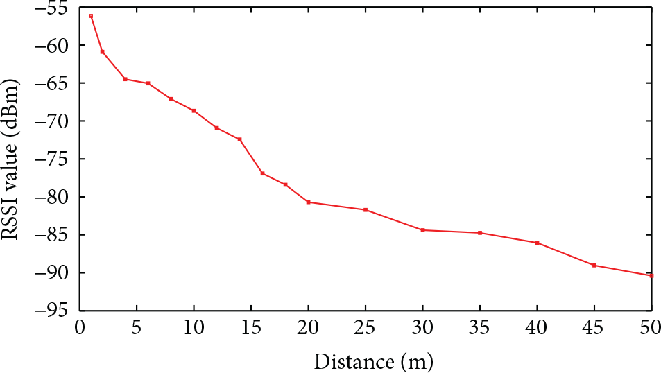
RSSI values for distances between two Zigbex motes.

In our localization method, we used the range technology which does not depend on the node density to estimate the distances between the mobile anchor and each unknown sensor. For each unknown sensor, the RSSIs from the mobile anchor at different neighboring locations were measured and converted to the estimated distances according to the mappings listed in Table 2.

We observed that the RSSI measurements between two sensors were usually oscillated around a center value. To show this phenomenon, in Figure 8, we depicted the distribution of RSSI measurements between two Zigbex sensors of distance 25 m. We also added the normal distribution curve which has the same mean and standard deviation as the RSSI distribution in Figure 8. It can be seen that the distribution of RSSI measurements is very similar to the corresponding normal distribution. This feature was also confirmed by the authors in [7, 18], although they used different communication chips to measure the RSSI values. Therefore, in the following, for simplicity, we will consider the RSSI distribution as a normal distribution.

Figure 8

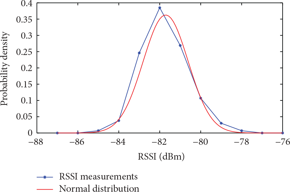
Distribution of RSSI measurements for distance 25 m and its corresponding normal distribution with the same mean and standard deviation.

It is known that, for the normal distribution, the values less than one standard deviation away from the mean account for 68% of the measured values, while two standard deviations from the mean account for 95% and three standard deviations account for 99.7%. Thus, in our experiment, we used the values of one, two, and three standard deviations as the maximum noises of the three error models for the distance estimation between the mobile anchor and each unknown sensor.

We used Table 2 to construct error models in subsequent simulation experiments. We randomly deployed unknown sensors and then measured the real distance between the mobile anchor and the unknown sensors. For error models 1–3, we added 1 to 3 standard deviations, respectively, as noise to the corresponding RSSI value and the linear interpolation is used to compute the estimated distances from the noised RSSI values. The linear interpolation is also used to compute the RSSI values for the distances which are not listed in the table and the standard deviation of the closest RSSI value is applied to each interpolated RSSI value.

The simulation environment for localization was as follows:

• (1)

Number of unknown sensors: 100.

(2)

Sensing fields:

• (a)

TGS (9 × 6, Figure 4(a)), Hilbert (fourth order, Figure 4(b)), and Gosper methods (level-3 node-Gosper curve, Figure 2(b)): the circle circumscribing each basic polygon (triangle, square, or hexagon) has a radius (r) of 10 m.

(b)

Random movement method (200 m × 200 m).

(3)

Number of anchors for the random movement method: 4.

(4)

Communication range of the mobile anchor for each method: random, $4r$ ; TGS, $\sqrt{3}r$ ; Hilbert, $3r$ ; and Gosper, $\sqrt{5}r$ .

(5)

Error models for the distance measurement between the mobile anchor and each unknown sensor: real distances plus 1 to 3 standard deviations (listed in Table 2).

(6)

Number of simulations: 100.

(7)

Range error = ((location error)/(communication range)).

(8)

Simulation tool: Matlab 2013a.

4.2. Localization Accuracy

Simulation results for the localization accuracy are shown in Figure 9.

Figure 9

(a) Location errors and (b) range errors in the random movement, TGS, Hilbert, and Gosper methods for different error models.

In the simulation, for each unknown sensor, we calculated the localization error for each method under three error models in which one to three times the standard deviation of the distance measurement between the mobile anchor and the unknown sensor are added to the real distance. As shown in Figure 9, the location error in the Gosper method (the proposed method) is almost identical to that in TGS and smaller than the location errors in the other two methods. Since the Gosper island can be triangularized, similar to TGS, for performing localization through trilateration, the localization results were similar to those of TGS. However, as shown in Table 1, under the same normalized sensing area, the Gosper method uses less number of radio broadcasts and travels shorter distance than those of TGS method.

The proposed method provided superior results compared with the Hilbert and random methods mainly because, on average, the anchor points in the Gosper method are closer to the unknown sensor in question compared with those in the other two methods. The range error of the proposed method was lesser than 0.0459 (approximately 4.6%), even for the case where three times the standard deviation was added to the real distances between the mobile anchor and the unknown sensors. This result is far superior to those of the localization methods involving static anchor nodes, such as the methods used in [3–6].

In [3], the authors proposed two static localization methods, named BLM (Bilateration Localization Method) and LSMLM (Least-Squares Multilateration Localization Method). Both methods used the hop-count technique to estimate the distances between the anchor node and each unknown node. The BLM used only two anchor nodes, and the LSMLM used up to 16 anchor nodes in order to increase the estimation accuracy. They claimed that the average range error of BLM is between 0.4 and 0.5 and it can be as low as 0.15 when LSMLS-16 (16-anchor nodes) is employed.

DV-Hop method, one of the renowned static localization methods, was proposed by Niculescu and Nath in [4]. According to the simulations reported in [4], the DV-Hop method demanded at least 20% of the sensors to be anchor nodes to improve the simulation results, and the average range errors were between 0.25 and 0.4 depending on the node density.

In [5], the authors proposed an algorithm named HCQ (hop-count quantization) to transform an integer hop-count to a real number hop-count based on the distribution of the given node's neighbors. The authors then used the transformed real number hop-count to solve the WSN localization problem with the MDS (multidimensional scaling) method. In their experiments, they used 5% of sensors as the anchor nodes, and for the case of random deployment of sensors, the range errors were between 0.2 and 0.8 depending on the node density.

In [6], the authors proposed a localization algorithm, called ellipse centroid localization algorithm, which combines the ellipse localization algorithm and the weighted centroid algorithm. In the proposed localization algorithm, for those unknown nodes that have at least two anchor nodes within their communication range, the ellipse localization algorithm was used to estimate their coordinates, and then the located nodes were extended as the anchors that increase the anchor density in the WSNs. Finally, the rest of unknown nodes were located by weighted centroid localization algorithm. In their experiments, they used 5% and 10% of sensors as the anchor nodes, and the range errors were 0.22 to 0.55 and 0.15 to 0.40, respectively, under various node densities.

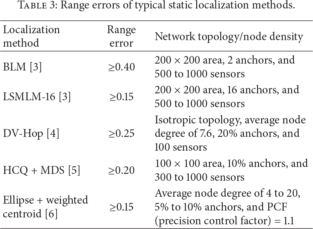
The range errors of the above static localization methods are summarized in Table 3. One can observe that all the range errors of these localization methods are larger than 0.15, which are much higher than that of our proposed localization method. The major reason our localization method has lower error rates than the static localization methods is that our method uses a mobile anchor to travel and stay at many locations (e.g., 343 locations in the level-4 node-Gosper island), which are evenly distributed within the sensing area, and to broadcast location messages to the unknown sensors. The mobile anchor staying at a specific location is, in fact, corresponding to a static anchor node located at that position for the static localization method. In general, the more the effective anchor nodes are used in a localization method, the higher the accuracy rate can be obtained by the localization method. Thus, our localization algorithm can have smaller range errors than those of the static localization methods.

Table 3

Range errors of typical static localization methods.

Localization method	Range error	Network topology/node density
BLM [3]	≥0.40	$\mathit{200}\times \mathit{200}$ area, 2 anchors, and 500 to 1000 sensors
LSMLM-16 [3]	≥0.15	$\mathit{200}\times \mathit{200}$ area, 16 anchors, and 500 to 1000 sensors
DV-Hop [4]	≥0.25	Isotropic topology, average node degree of 7.6, 20% anchors, and 100 sensors
HCQ + MDS [5]	≥0.20	$\mathit{100}\times \mathit{100}$ area, 10% anchors, and 300 to 1000 sensors
Ellipse + weighted centroid [6]	≥0.15	Average node degree of 4 to 20, 5% to 10% anchors, and PCF (precision control factor) = 1.1

4.3. Energy Consumption for the Mobile Anchors

We measured the energy consumption of the mobile anchors in the routing protocols of the random, TGS, Hilbert, and Gosper methods. We used a simple model, similar to that used in [19], for describing the radio energy dissipation; in the model, the operation of the radio and power amplifier accounts for the energy consumed by the transmitter, and the energy consumed by the receiver is used for radio operation. Suppose that the distance between the sender and the receiver is d and that there are k bits to be transmitted. The power dissipation formulas are

$$\begin{array}{cc}& E_{\mathrm{T}\mathrm{X}}\left(k,d\right)=\left\{\begin{array}{cc}k{E}_{\mathrm{e}\mathrm{l}\mathrm{e}\mathrm{c}}+k{\epsilon }_{fs}{d}^{\mathrm{2}},\hfill & d<d_{\mathrm{0}}\hfill \\ k{E}_{\mathrm{e}\mathrm{l}\mathrm{e}\mathrm{c}}+k{\epsilon }_{mp}{d}^{\mathrm{4}},\hfill & d\ge d_{\mathrm{0}},\hfill \end{array}\right.\\ E_{\mathrm{R}\mathrm{X}}\left(k\right)=E_{\mathrm{e}\mathrm{l}\mathrm{e}\mathrm{c}}\times k,\end{array}$$

(10)

where $E_{\mathrm{T}\mathrm{X}}\left(k,d\right)$ and $E_{\mathrm{R}\mathrm{X}}\left(k\right)$ are the power consumed by the transmitter and receiver, respectively. Furthermore, $E_{\mathrm{e}\mathrm{l}\mathrm{e}\mathrm{c}}$ is the energy consumed per bit by the transmitter or receiver circuit, and ${\epsilon }_{fs}{d}^2$ or ${\epsilon }_{mp}{d}^4$ is the amplifier energy that depends on the transmitter amplifier model used. The parameter $d_0$ is set to $\sqrt{{\epsilon }_{fs}/{\epsilon }_{mp}}$ , which is the power consumption threshold.

In addition to the energy consumption for radio broadcasts, we also considered the movement of a mobile car and its restarting cost at each stop. All the additional parameters required in the simulation of energy consumption are presented in Table 4.

Table 4

Additional simulation parameters.

Parameters	Values
k (location package size)	100 bits
$E_{\mathrm{e}\mathrm{l}\mathrm{e}\mathrm{c}}$ (the energy dissipated per bit)	50 nJ/bit
${\epsilon }_{fs}$ (amplifier energy for distance square)	10 pJ/bit/m2
${\epsilon }_{mp}$ (amplifier energy for distance quartic)	0.0013 pJ/bit/m4
v (velocity of mobile anchor)	3 m/sec
$E_v$ (energy consumption for mobile anchor under velocity  v)	0.003 J/sec
$E_{\mathrm{m}\mathrm{o}\mathrm{t}\mathrm{o}\mathrm{r}}$ (energy consumption when restarting the motor of mobile anchor each time)	0.005 J

The energy consumption of the mobile anchor was determined by three factors: number of radio broadcasts, distance traveled, and number of times the mobile car stopped and started. The simulation results are presented in Figure 10. The sensing areas are normalized to 1000 m² for each method. As shown in Table 1, the node-Gosper curve requires the least number of radio broadcasts and is the shortest routing path for a given normalized area. Therefore, Gosper method consumed the least energy among the four methods.

Figure 10

Energy consumption of the mobile anchors in the four localization methods (sensing areas are normalized to 1000 m²).

5. Conclusions

We propose a mobile anchor localization method involving a node-Gosper curve as the routing path, for WSNs. We showed that, for a given area, both the length and number of turning points of the node-Gosper curve are smaller than those of the Hilbert and TGS curves. Consequently, the energy consumption of a mobile anchor that uses a node-Gosper curve as the routing path is less than that of a mobile anchor using the other two curves.

Experiment results of the localization simulations showed that the range error of the proposed method was less than 4.6%, which makes the method superior to those involving random, TGS, and Hilbert paths, and far superior to several existing static localization methods for WSNs, such as the methods used in [3–6].

To calculate the center coordinates of each hexagon in the Gosper island, we proposed two addressing schemes—ring-based and base-7 addressing schemes—for the hexagonally tessellated plane and determined their properties. The ring-based addressing scheme can be used to efficiently calculate the Cartesian coordinates for the center point of any hexagon in the Gosper island. Hopefully, the new properties of the two addressing schemes exploited in this study can facilitate the procedures of image processing based on the hexagonal coordinate systems, such as the works in [15, 20–22].