
Abstract
The high outage probability of an underwater wireless sensor may lead to high energy consumption. How to reduce the outage probability should be considered for underwater acoustic sensor networks (UASNs), where battery change is very difficult. Power control, which is one of the technologies to effectively reduce the outage probability, has also been developed for UASNs. However, when using the power control method with the maximum power to transmit packets, the slow fading of the signal in UASNs leads to serious accumulative interference in the receiver, which in turn leads to an even higher outage probability. Another challenge in UASNs is the complex acoustic channel condition with time-space-frequency variation and uncertain TL, which make it difficult to obtain the channel status information (CSI). To address these issues, a novel partial power control (PPC) algorithm based on outage probability minimization in UASNs is proposed. The proposed algorithm captures transmission loss (TL) using the Markov chain Monte Carlo (MCMC) method and estimates CSI in the next moment using AR prediction. The simulation results show that the proposed algorithm can effectively reduce the accumulative interference to the receiver and then reduce the outage probability by 19.3% at the maximum.
1. Introduction
During the past decade, underwater acoustic sensor networks (UASNs) have attracted significant interest from academia and industry because of a wide range of applications, including underwater environment monitoring, offshore structural health monitoring, target tracking, and oceanography data collection [1–3]. Thus, in applications for UASNs, energy conversation needs to be taken into more consideration because battery replacement or recharging is very difficult in the deep ocean [4]. Power control, which is one of the key technologies to effectively reduce energy consumption, has been developed in UASNs [5]. For example, the water-filling power control (WFPC) method is a well-known method and has wide applications for land. For a single user, fading channel WFPC can maximize the expected rate, and it is optimal for increasing the transmission power as a function of the instantaneous channel quality. In other words, when channel conditions are good, more power and a higher data rate are sent over the channel. As the channel quality degrades, less power and a smaller rate are sent over the channel. If the instantaneous SNR falls below the cutoff value, the channel is not used [6–8]. Therefore, WFPC can reduce the energy consumption. However, these classic power control methods directly applied for underwater appear less beneficial because of more differences between UASNs and wireless sensor networks (WSNs), such as the uncertain transmission loss (TL), high accumulation interference in the receiver, and high outage probability.
Specifically, in UASNs, power control methods face the following challenges. (1) In UASNs, the velocity of underwater sound propagation is 1500 m/s, which is five orders of magnitude less than that of the radio frequency [9]. The slow fading of the signal brings more accumulation interference in UASNs than that on land. If the transmitter sends data with the maximum power, the accumulation interference in the receiver is serious. Thus, the higher the outage probability, the more the energy consumption. Therefore, it is important for the power control method in UASNs to reduce accumulation interference. (2) The uncertainty of TL brings power control great challenges. The underwater acoustic channel is one of the most complex channels so far and is affected by uncertainty in the environment factors, such as weather, ocean current, seabed, and shipping [10]. Therefore, it is hard for UASNs to capture TL. Studies on capturing the uncertainty of TL are still being conducted. Even less work has been done to study the relationship between TL and power control in UASNs. Without capturing TL, it is difficult to characterize the channel statistics, such as the probability distribution and time-coherence properties, which are important for the design of power control in UASNs. To address this issue, the partial power control (PPC) algorithm based on outage probability minimization in UASNs is proposed.
The contributions in the paper are as follows. (1) The PPC algorithm can analyze the accumulative interference of randomly deploying nodes by building the accumulative interference model and can reduce the accumulative interference by adjusting the power control factor. Therefore, the PPC algorithm can effectively reduce the outage and retransmission probability, save energy consumption, and improve the network capacity. (2) The PPC algorithm can capture TL using the MCMC method and adjust the transmission power according to the estimation of the AR prediction. Therefore, the PPC algorithm can adjust the transmission power to effectively reduce energy consumption.
The remainder of this paper is structured as follows. We discuss related work of power control in Section 2. In Section 3, the PPC algorithm based on outage probability minimization is described. In Section 4, the method to obtain reliable CSI is described. In Section 5, the numerical simulations are discussed. We conclude with our conclusions in Section 6.
2. Related Work
Power control is widely used in terrestrial wireless sensor networks such as the water-filling power control (WFPC) algorithm and the channel inversion power control (CIPC) algorithm [11]. However, most of these power control methods on land do not apply directly for UASNs. For example, the intuition behind WFPC is to take advantage of good channel conditions. When channel conditions are good, more power and higher data rates are sent over the channel. Therefore, WFPC on land can effectively reduce energy consumption and take the channel capacity into more consideration. However, because a higher outage probability will lead to more retransmission and higher energy consumption, it is important for WFPC in UASNs to take into consideration outage probability minimization as well as the capacity. In [12], the channel inversion power control algorithm for user equipment (UE) uses the truncated channel inversion power control policy with a cutoff threshold for the outage probability and spectral efficiency. Based on outage probability minimization, the CIPC algorithm can reduce energy consumption. However, because there are a lot of uncertainties in the transmission loss (TL) for UASNs, it is hard to obtain feedback from the receiver, which may lead to a higher outage probability.
In UASNs, there are many power control algorithms applied widely. In [13], joint power and rate control with constrained resources for underwater acoustic channels is proposed, and it adjusts the transmission power and the number of coded packets to obtain the average energy per bit minimization. For the optimization, Ahmed and Stojanovic impose the following two constraints: (1) the transmitter power should be within a maximum available power and (2) the number of coded packets should not exceed a maximum value. This method can adaptively reduce the transmission power according to the CSI. For UASNs, there is a scene in which many transmitters with the same power send data to the sink. Then, the sink will accumulate more interference because of the slow fading of signal, which will lead to a high outage probability.
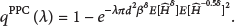
In [14], Qarabaqi and Stojanovic give an adaptive power control (ADPC) method for underwater acoustic communication. This method relies on feedback to inform the transmitter of the present channel state. In this method, the transmitter can estimate the CSI in the next moment by AR prediction method and adjust its power accordingly. This method can adaptively adjust the transmitter power and reduce energy consumption. It is a linear and conversional method for AR prediction to obtain the CSI at the next moment. However, for UASNs, there is uncertain TL. It is difficult to estimate the CSI in the next moment by AR prediction. As shown in Figure 1, an uncertain TL will cause huge variation. The TL has uncertain features that are caused by weather, ocean current, seabed, shipping, and so forth. Affected by an uncertain TL, the fluctuation of the sound source level (SL) and noise level (NL) is ±5 dB, and the variation range of the SL transmission distance varies from 25 km to 130 km. There is a 105 km difference from 25 km to 130 km. It is difficult to estimate the CSI in the next moment because of the higher variation of the TL. To address this issue, the Markov Monte Carlo method is used in this paper. The Markov chain Monte Carlo (MCMC) method is used to first sample the probability distributions of the geoacoustic parameters. Unlike previous research [15], the results of the geoacoustic inversion are only an intermediate goal. Subsampling of the multidimensional model parameter distribution is then used to map parameter uncertainties to the TL domain [16]. The MCMC method can obtain the confidence intervals (CI) of the TL. Based on the CI of the TL, the AR prediction method is used to estimate the CSI in the next moment. Therefore, the PPC algorithm can obtain reliable CSI.
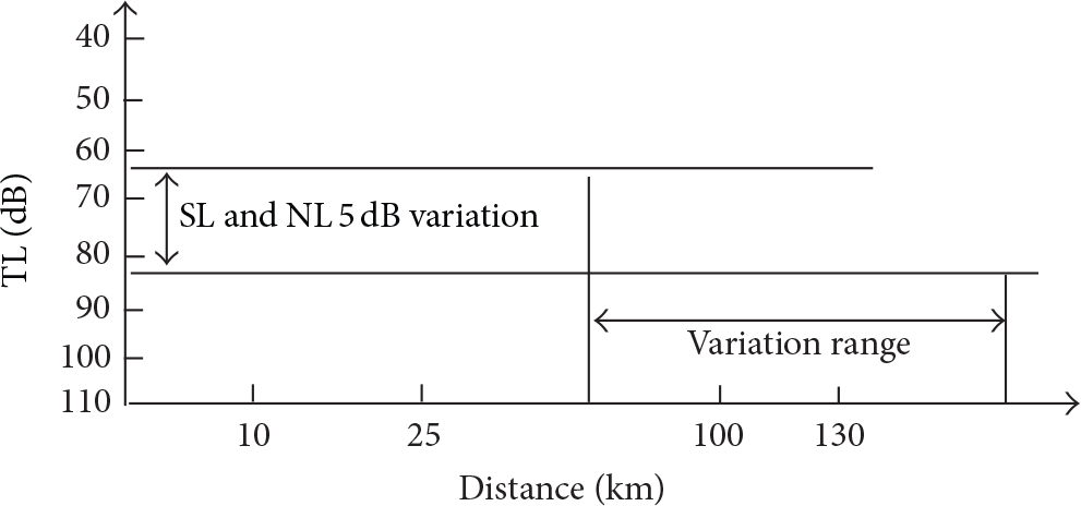
Uncertain TL will bring huge variation.
To summarize, PPC algorithms can analyze the accumulative interference, reduce the outage probability, obtain reliable CSI, and improve the network capacity.
3. PPC Based on Outage Probability Minimization
The PPC algorithm in this paper establishes a space accumulative interference model by using stochastic geometry, analyzes the accumulative interference of receiver, and then, based on the minimum outage probability, deduces the power control formula. The power control formula is related to the CSI. Because of the uncertain TL, it is difficult to obtain reliable CSI. To address the issues, in this paper, the MCMC method is used to capture the TL, and the AR prediction method is used to predict the CSI at the next moment. In general, the PPC algorithm can reduce energy consumption and improve the network capacity.
3.1. Space Accumulative Interference Model
The network is viewed at a single snapshot in time for the purpose of characterizing its spatial statistics. Every potential
Assume that, at the time of t, the transmitting nodes (
As shown in Figure 2, the model
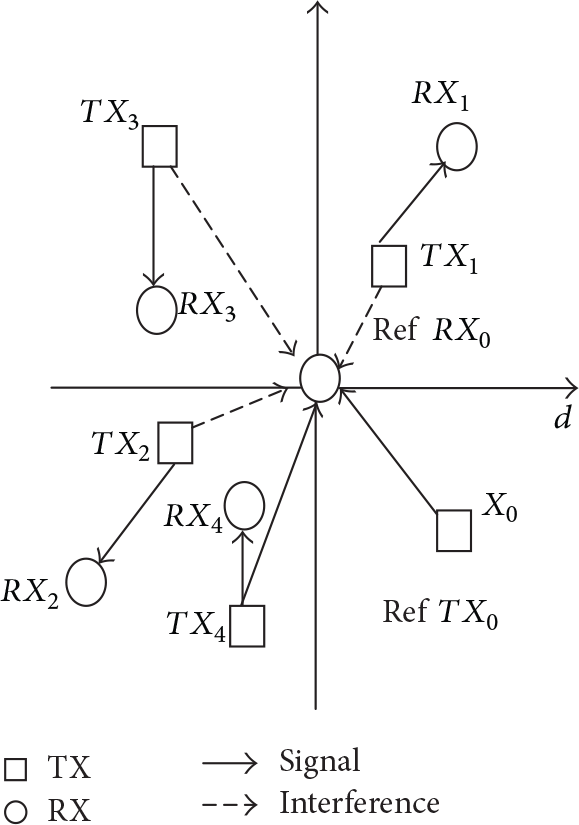
Accumulative interference model of UASNs.
The random

In the formula,
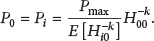
When
This formula means that the ith node transmission power is a certain proportion to the maximum power. The proportion is the ratio of any channel status distribution
3.2. The Outage Probability and Network Capacity
To prove that the PPC can minimize the outage probability, we deduce the formula of the outage probability and network capacity. According to the above space accumulative interference model, the approximate formulas of outage probability minimization and network capacity maximization are as follows.
According to formula (1), when the SINR falls below a prescribed threshold β, there is the outage probability formula as follows:

β is the SINR received threshold. Putting formula (2) into formula (3), the outage probability formula changes as follows:

When

Formula (5) is the final outage probability formula. From formula (5), we know that the outage probability is related to the transmission distance d, SINR β, and channel status distribution mean
The network capacity is defined as the total number of successful transmissions in a unit area when the outage probability is limited:
Compared with the outage probability at
(1) When

When
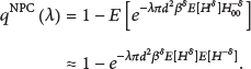
The formula of the network capacity with the maximum power is
Using NPC, from formula (8), we know the relationship between the outage probability and interference as well as the fading of the channel. In other words, the higher the user intensity, the higher the accumulative interference under the limit areas. The higher the accumulative interference and the fading of the channel, the higher the outage probability. Therefore, reducing the outage probability is key for the PPC.
From formula (9), we know that there is the relationship between the capacity network and the fading of the channel under the limit of the outage probability. The capacity network varies as the fading of the channel. Therefore, to improve the capacity of the network, knowledge of reliable CSI with the MCMC and AR methods is needed.
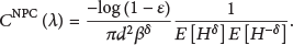
(2) When
Therefore, comparing the approximate formula to formula (8), the outage probability formula of the CIPC is the same. Comparing the formula with formula (9), the network capacity formula of the CIPC is the same. That is, the formulas are the same when
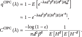
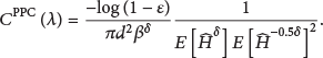
(3) When

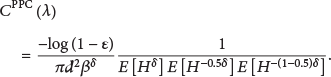
From formula (11), we know that there is a relationship between the outage probability and the fading of the channel. Compared to the fading of the channel of the NPC and ICPC, the fading of the channel in the PPC is minimized. That is, there is outage probability minimization for the PPC.
Comparing the formula with formula (8), there is a difference within the CSI. When

When

By using Holder's inequality, we can prove that
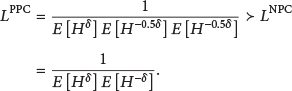
Combine formulas (15), (8), and (11), due to
Combine formulas (15), (9), and (12), if
Therefore, compared with the NPC algorithm, the PPC algorithm can obtain outage probability minimization and network capacity maximization.
When
4. Capturing the TL Using the MCMC Method and Estimating the CSI Using AR Prediction
According to formula (11), we know that the formula of the outage probability is related to the CSI. It is important for power control to estimate the CSI. Because of the uncertain TL and complex channel status, it is difficult to estimate the CSI. To address this issue, the MCMC method is used to capture the TL, and the AR prediction method is used to estimate the CSI at the next moment. The PPC algorithm can obtain reliable CSI to improve the power control.
4.1. MCMC Method
The uncertainty of the TL is the acoustic properties in the ocean, which cannot be completely accurately forecasted, measured, or analyzed because of a lot of factors, such as weather, ocean current, seabed, and shipping. Therefore, in UASNs, acquiring the CSI is challenging. Studies on capturing the TL are at the developing stage. In [19], the MCMC method captured the TL at some distance. The Markov chain Monte Carlo (MCMC) method contains two parts, MC (Monte Carlo integration) and the MC (Markov chain). The MCMC method is used to solve the parameter expectations in a complex environment, which cannot be directly calculated. The mapping process is as shown in Figure 3 in which there is U (usage domain), D (data domain), and M (environment domain).
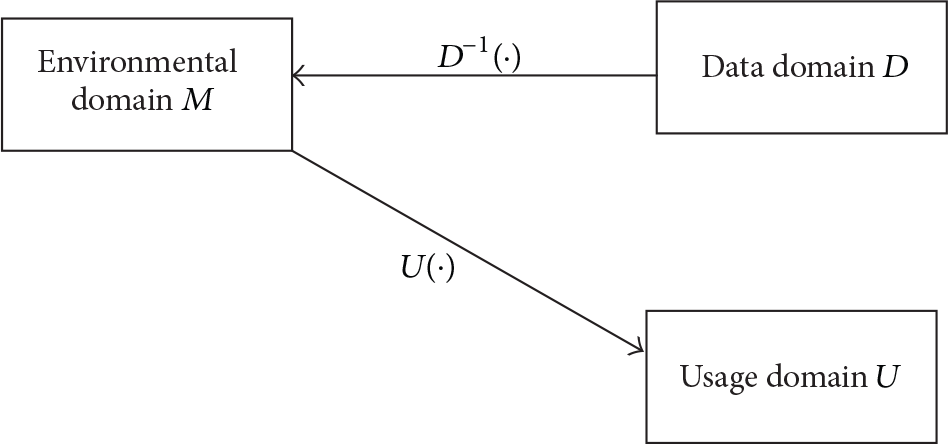
The mapping process.
The acquisition method of capturing the uncertainty value in the MCMC method is that we collect data (data domain D) by hydrophone arrays, respectively, map the data into various models (environmental domain M) (such as the deep-sea-channel model, shallow-channel model, sound velocity model, noise model, reverberation model, and signal model; these models are collectively defined as the environmental domain model M), and integrate the distribution of the usage domain U in the data domain D. The usage domain U is at a certain distance CI of the TL, written as
4.2. Estimation of CSI Based on the AR Prediction Method
After capturing the TL at a certain distance, the AR prediction method is used to estimate the CSI in order to obtain reliable CSI and improve the power control.
The AR prediction method is a linear estimation in which data after the Nth moment will be obtained based on data before the Nth moment. That is, based on historic statistics data, we can estimate the data at the next moment.
After the AR prediction, the CSI at the next moment is rewritten as
Put
The formula for network capacity maximization is
5. Results and Discussion
5.1. Capturing TL
The MCMC method is used to capture the TL. There are 160,000 sample points in Monte Carlo method in a 2 km transmission distance, and then, the sample points will be mapped M (such as the deep-channel model, shallow-channel model, sound velocity model, noise model, reverberation modeling, and signal models). The posterior probability

Capturing the TL by the MCMC method.
5.2. Estimation of CSI Based on the AR Prediction Method
After capturing the TL, we will estimate the CSI at the next moment using the AR prediction method. From Figure 5, we know the relationship between the probability distribution of the TL and transmission range. According to

Estimation of CSI based on the AR prediction method.
5.3. Outage Probability and Network Capacity When
If the transmitter sends data with maximum power (when
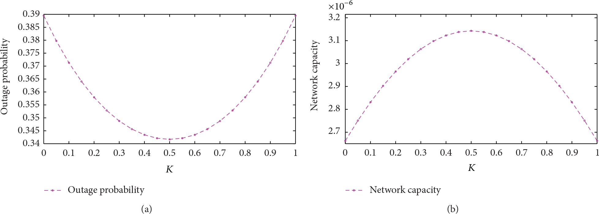
(a) Outage probability versus K. (b) Network capacity versus K.
5.4. The Outage Probability and Network Capacity of the PPC Algorithm with the Variation of the Parameters α and λ
When α varies from 1 to 2 (in other words, the transmission varies from cylindrical transmission in the shallow sea to spherical transmission in the deep sea), the fading of accumulative interference is shown in Figure 7. When

Fading slowness of the accumulative interfering versus α.
As shown in Figure 8, the outage probability varies with λ from 1/km2 to 100/km2, and we can obtain outage probability maximization when

Outage probability versus K.
5.5. Comparing the Outage Probabilities in the PPC, NPC, and WFPC Algorithms
As shown in Figure 9, the outage probability varies with transmission distance. The higher the transmission distance, the greater the outage probability. The outage probability based on NPC is high, and the outage probability of WFPC is moderate. The outage probability of ADPC and PPC is low. The PPC algorithm can obtain outage probability minimization because PPC takes the TL and accumulative interference in the receiver into consideration. NPC suffers from a high outage probability because of the greater accumulative interference in the receiver. Compared to the outage probability with the NPC algorithm, the outage probability of the PPC algorithm decreases approximately 19.3% at the maximum level. Compared with ADPC, PPC can obtain a low outage probability because of the captured TL by the MCMC method and estimated channel of the next moment by AR prediction.

Comparison between the NPC, WFPC, ADPC, and PPC algorithms.
As shown in Figure 10, when
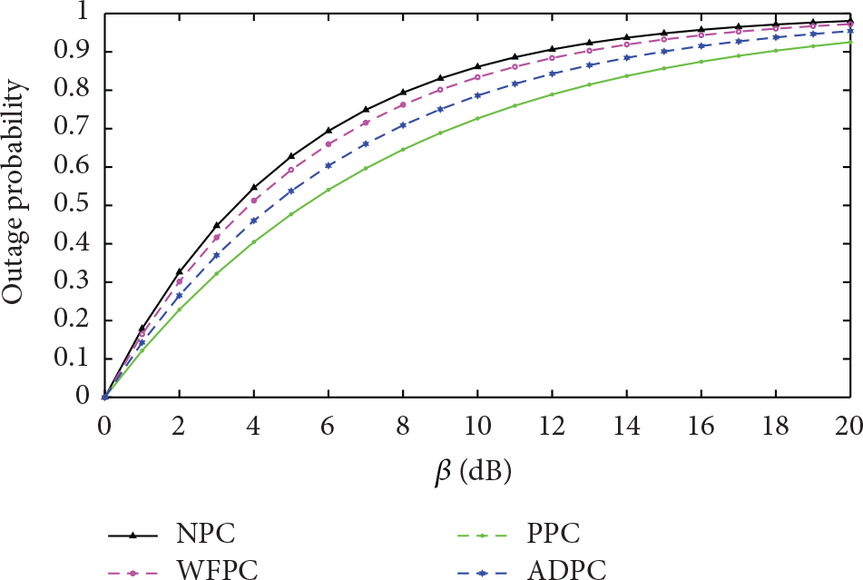
β versus the outage probability.
5.6. Effective PPC
As shown in Figure 11, PPC can adjust the effective power according to the estimation of CSI. Data are correctly received under the premise of effective channel compensation. Figure 11 shows that PPC can obtain reliable CSI at the next moment, which effectively compensates for channel attenuation. According to the CSI that reflects good channel status, more power is used. Therefore, the PPC algorithm in this paper can effectively reduce energy consumption by reducing the outage probability and obtaining reliable CSI compared to the NPC algorithm. The PPC algorithm can save energy consumption by a maximum of 11.5%.
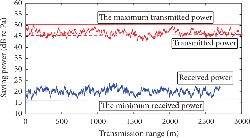
Adaptive PPC algorithm.
6. Conclusion
In UASNs, there are some features that have affected power control, such as the time-space-frequency acoustic channel, serious accumulative interference, and an uncertain TL. To overcome these difficulties, we have proposed the PPC algorithm based on outage probability minimization. The PPC algorithm uses stochastic geometry theory to establish a spatial accumulative interference model, which aims to establish the relationship between outage probability minimization and power control. To obtain the CSI, the PPC algorithm uses the MCMC method to capture the TL and uses the AR prediction method to estimate the CSI at the next moment. The simulation results show that the MCMC method can obtain 91% CI of the uncertain TL and that the AR prediction method can effectively estimate the CSI. The PPC algorithm can reliably achieve outage probability minimization and network capacity maximization. Compared to NPC, the PPC algorithm reduces the outage probability by 19.3% and saves energy consumption by a maximum of 11.5%.
Footnotes
Competing Interests
The authors declare no competing interests.
Authors' Contributions
Yun Li, Yishan Su, Zhigang Jin, and Sumit Chakravarty contributed equally to this work.
Acknowledgments
This work was supported in part by the following projects: the National Natural Science Foundation of China through Grant 61571318, Qinghai Science and Technology Project 2015-ZJ-904, the Guangxi Nature Science Fund (2015GXNSFAA139298), the Guangxi Experiment Center of Information Science (KF1406), and the Opening Project of Guangxi Colleges and Universities Key Laboratory of Unmanned Aerial Vehicle (UAV) Telemetry (WRJ2015ZR01).