Sage Journals: Discover world-class research

Abstract

A routing-benefited deployment algorithm combining static and dynamic layouts is proposed, and its comprehensive performance evaluation is given in this article. The proposed routing-benefited deployment algorithm is intended to provide a suitable network deployment and subsequent data transmission approach for underwater optical networking and communication. Static nodes are anchored for long-term monitoring, and movable nodes can adjust their depths based on the virtual force and move with the variation of area-of-interest changing. Then, nodes begin to collect data that they can monitor and transmit to sink nodes. Here, the underwater wireless optical communication model is described to actualize the real environment, and the vector-based forwarding protocol is particularly considered to compare the impact of different deployment algorithms on routing. It is shown by simulation experiment results that routing-benefited deployment algorithm outperforms several existing traditional virtual force deployment algorithms in terms of coverage, lifetime, energy consumption balance, packet-loss rate, and time-delay.

Keywords

Underwater optical wireless network static and dynamic layouts routing virtual force performance evaluation

Introduction

Underwater wireless sensor networks (UWSNs) are composed of homogeneous and/or heterogeneous sensor nodes. These nodes have the functions of data acquisition, processing, and wireless communication, which can be increasingly available for marine environment monitoring, disaster alarm and pollution detection, ocean resource exploration and exploitation, and military supervision.^1,2

UWSNs have many differences from terrestrial sensor networks. First, the UWSNs are three-dimensional (3D) rather than two-dimensional (2D) networks.³ Second, the underwater environment is complicated and fickle, and there are various disturbances such as ocean currents, marine life, seawater salinity, and temperature/pressure, which will seriously affect the performance of communication and networking.⁴ Third, underwater is an untouchable and rugged environment. In this case, energy becomes a vital resource because changing batteries seems impossible.⁵ In addition, the cost of underwater nodes is extremely high, which poses huge challenges to the deployment of UWSNs.⁶

The deployment approaches not only assign the spatial positions of varying types of sensor nodes but also design the topology, even architecture of networks. Therefore, network deployment is a determinant of energy consumption, and the capacity and reliability of networks.⁷

The deployment of underwater network nodes is divided into static deployment and dynamic deployment. Static deployment is simple and efficient, but it is only suitable for monitoring the fixed areas. The dynamically deployed nodes can adjust positions spontaneously to improve coverage ratio and connectivity ratio, but the cost of this kind of deployment is high and the mobile energy consumption is huge.⁸ Therefore, the combination of static and dynamic deployments is more suitable for the actual situation of UWSNs, which can not only save energy consumption, prolong the network lifetime but also economize costs and improve robustness.

Regarding communication methods, the channels in UWSNs mainly include electromagnetic wave–based, acoustic wave–based, and optical wave–based ones. Since seawater contains salt which is a conductive transmission medium, the electromagnetic signal can only propagate for a short distance.⁹ Besides, underwater wireless optical communications can implement several orders of magnitude higher propagation speed, lower time-delay, lower data-rate, and higher bandwidth than underwater acoustic communications.^10–12 Therefore, optical channels are more suitable for high-speed, multi-service UWSNs.¹³

Moreover, for the performance evaluation of network deployment methods, the current papers mainly consider the coverage and energy consumption performance of the network. Network deployment also greatly affects routing performance such as packet-loss rate (PLR) and time-delay.

Hence, this article proposes a routing-benefited underwater wireless sensor network deployment algorithm (RBDA). Some nodes are static nodes for long-term monitoring. The other nodes are movable, and they move in depth with the altering of area-of-interest according to the virtual force. The main contributions in this article include the following:

A deployment algorithm based on underwater wireless optical communication mode is proposed, which takes into account sunlight background noise and optical transmission loss model to make it more suitable for practical application scenarios.

Considering the network routing process, the VBF (vector-based forwarding) protocol is introduced, and routing performance is employed as one of the evaluation indicators of the deployment method.

The performances of the proposed RBDA, including network coverage (including its convergence speed), lifetime, energy consumption balance, PLR, and time-delay are evaluated and compared with some existing deployment algorithms.

The rest of this article is organized as follows. Section “Related work” provides a brief review of existing underwater deployment algorithms based on different methodologies. Some related preliminaries are outlined in section “Preliminaries.” A hybrid deployment algorithm with static and movable sensor nodes is proposed in section “Algorithm description.” The performance analysis and simulation of our deployment approach and the comparison with the existing several other methods are shown in section “Simulation results and discussion.” The summary and prospects are conducted in section “Conclusion.”

Related work

Regarding the current deployment approaches of UWSNs, they can be categorized into static and dynamic ones according to whether the nodes can move.

The core idea of the static deployment scenarios is using convex polyhedron to fill 3D space. Alam and Haas¹⁴ used four polyhedrons, namely, cube, hexagonal prism, rhombic dodecahedron, and truncated octahedron to fill the 3D area. They proposed several useful definitions, such as volumetric quotient and sensing range. Then, they proposed the concept of cell and duty-cycled scheme to extend the lifetime of the networks in Alam and Haas.¹⁵ Liu¹⁶ further proposed a cluster-based deployment algorithm based on the aforementioned method.

The deployment methods of dynamic nodes can be designed based on graph theory, virtual force, and artificial intelligence, etc.¹⁷ Among them, data centers are required to instruct other nodes in graph theory–based deployments, so it is difficult to achieve complete distributed deployment. Also, artificial intelligence methods tend to be complex in calculation. In contrast, the virtual force–based methods can ensure the distributed deployment of nodes, and the complexity is low. Therefore, they are more suitable for UWSNs composed of battery-powered nodes.

Zou and Chakrabarty¹⁸ first introduced the theory of virtual force to the deployment to 3D environments and verified the feasibility. Li et al.¹⁹ rewrote the virtual force formula, and introduced central gravity and balance force to jointly optimize the movement of nodes. Boufares et al.²⁰ gave a feasible method to derive the distance threshold for 3D deployments based on virtual force. Liu et al.²¹ continued to improve the formula of virtual force and introduced the mobile benefit model to balance the energy consumption.

Most of the deployment algorithms for UWSNs are based on acoustic networks; there are only a few pieces of research works on the deployment of underwater optical wireless sensor networks. Xing et al.²² and Wang et al.²³ proposed two types of underwater acoustic-optical hybrid wireless networks’ architectures, where the deployment of surface gateway nodes is focused in Xing et al.,²² and the network transmission protocols are concerned in Wang et al.,²³ respectively. Yadav and Kumar²⁴ designed a clustering approach for UWSNs which combined the acoustic, optical, and electromagnetic wave–based communication techniques, but the placement of nodes merely obeys a 2D Gaussian distribution.

Preliminaries

Underwater optical wireless communication model

The underwater wireless optical communication system is briefly shown in Figure 1. The electrical signal to be transmitted is modulated onto a light source (LD or LED) to output an optical signal. Next, the optical signal is transmitted through the underwater channel to the receiver, then converted into an electrical signal by photo-detector (PD), at last, recovered by the demodulator.^25,26

Figure 1.

Schematic diagram of underwater wireless optical communication system.

Assuming that the power of the optical signal emitted by the light source of the optical transmitter is P_t and the optical power of the signal received by the PD is P_r. Their functional relationship can be expressed as

P_{t} = \frac{2 π d^{2} \cos φ \sin^{2} θ}{η_{t} η_{r} A_{r}} e^{k (λ) d} P_{r}

(1)

where d is the distance between the transmitter and the receiver. θ (half-angle beam width) and φ (angle between the optical axis of the receiver and the connection between the transmitter and receiver) are shown in Figure 1. η_t and η_r denote the optical efficiency of transmitter and receiver, respectively. A_r indicates the aperture area of the receiver, and k(λ) symbolizes the attenuation coefficient, which is influenced by the wavelength of the optical signal λ, as well as the general turbidity of the water.

The PD converts the optical power P_r to photocurrent i

P_{r} = \frac{i}{ℜ}

(2)

where ℜ is the responsivity of PD, and it can be defined as

ℜ = \frac{η_{PD} q λ}{ℏ c}

(3)

where η_PD denotes the quantum efficiency of PD, q indicates the electron charge, ħ is the Planck constant, and c represents the propagation velocity of light in vacuum.

Substituting equations (2) and (3) into equation (1), then

P_{t} = \frac{2 π q η_{PD} λ i d^{2} \cos φ \sin^{2} θ}{ℏ c η_{t} η_{r} A_{r}} e^{k (λ) d}

(4)

Also, the signal-to-noise ratio (SNR) for the underwater optical wireless communication system can be expressed as

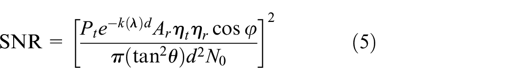
SNR = {[\frac{P_{t} e^{- k (λ) d} A_{r} η_{t} η_{r} \cos φ}{π (\tan^{2} θ) d^{2} N_{0}}]}^{2}

(5)

where N₀ is the noise equivalent power, composed of solar background shot noise power (N_b), signal shot noise power (N_s), dark current noise power (N_d), and preamplifier noise power (N_p), that is

N_{0} = \sqrt{N_{b}^{2} + N_{s}^{2} + N_{d}^{2} + N_{p}^{2}}

(6)

where the value of N_b changes with the depth of the receiver in water D, the wavelength, and power of the emitted optical signal. The value of N_s also changes with the wavelength and power of the transmitted optical signal. N_d and N_p can be regarded as constants in the simulation for the sake of simplicity since they are not affected by the transmitter, receiver, and the transmitting signal.²⁷

Applying the Shannon theorem based on known system bandwidth (W) and SNR, the data transmission bit rate (R_b) can be attained. Then, the optical energy E_t consumed by each transmitter for transmitting each symbol (bit) is

E_{t} = \frac{P_{t}}{R_{b}} = \frac{P_{t}}{W \cdot \log_{2} {1 + {[\frac{P_{t} e^{- k (λ) d} A_{r} η_{t} η_{r} \cos φ}{π (\tan^{2} θ) d^{2} N_{0}}]}^{2}}}

(7)

where P_t can be calculated by equation (4).

3D virtual force model

The basic mechanism of virtual force is that a repulsive force will be produced when two neighbor nodes are close to each other, or an attractive force will be produced when two neighbor nodes are far away from each other. In this case, nodes can adjust the distances between their neighbors and themselves to optimize spatial distribution and coverage performance of the whole network. The preinstall threshold for judging whether the distance between neighbor nodes is close or far is recorded as d_th.

The coordinates of n_i and n_j are (x_i, y_i, z_i) and (x_j, y_j, z_j), respectively, and the virtual force exerted by sensor n_j on sensor n_i is expressed as

F_{ij} = {\begin{matrix} K_{r} \frac{1}{d_{ij}} \cdot v 0 < d_{ij} < d_{th} \\ - K_{a} (d_{ij} - d_{th}) \cdot v d_{th} \leq d_{ij} \leq r_{c} \end{matrix}

(8)

where r_c is the communication radius of the node, K_r and K_a represent the repulsive coefficient and the attractive coefficient, respectively. d_ij represents the Euclidean distance between the two nodes. v is a 3D vector, which represents the direction of the virtual force as

v = \frac{(x_{i} - x_{j}, y_{i} - y_{j}, z_{i} - z_{j})}{d_{ij}}

(9)

In practical terms, realizing the 3D free movement of the nodes is too costly; it is more of engineering significance to assume that the nodes can only adjust their depths.²⁸ Hence, the moving distance is directly related to the projection of the virtual force in the vertical direction. α_ij is introduced as

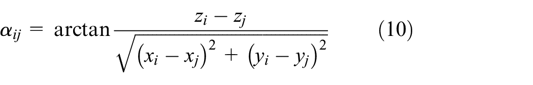
α_{ij} = \arctan \frac{z_{i} - z_{j}}{\sqrt{{(x_{i} - x_{j})}^{2} + {(y_{i} - y_{j})}^{2}}}

(10)

and then, the projection of virtual force in vertical direction exerted by sensor n_j on sensor n_i is

F_{ij}^{'} = {\begin{matrix} K_{r} \frac{1}{d_{ij}} \sin α_{ij} z 0 < d_{ij} < d_{th} \\ - K_{a} (d_{ij} - d_{th}) \sin α_{ij} z d_{th} \leq d_{ij} \leq r_{c} \end{matrix}

(11)

Besides the virtual force between nodes, when the node is close to the upper or lower boundary, a repulsive force can be also produced to prevent it from moving out of the monitoring space. The direction of this type of repulsive force is away from the boundary, and its magnitude is

| F_{b i} | = {\begin{matrix} K_{b} \cdot (d_{bi} - d_{bth}) 0 \leq d_{bi} < d_{bth} \\ 0 d_{bi} > d_{bth} \end{matrix}

(12)

where K_b is the repulsive coefficient of the boundary, d_bth is the threshold distance determining whether the repulsive force will be exerted, d_bi is the depth difference between node n_i and the closest boundary of the monitoring area.

According to equations (11) and (12), the total virtual force exerted on n_i is

F_{i} = \sum_{j = 1, j \neq i}^{N} F_{ij}^{'} + F_{b i}

(13)

where N is the total number of nodes.

The node moves upward and downward under the virtual force, the distance and direction of movement are

l_{i} = β ω l_{max} F_{i}

(14)

where l_max is the preinstall maximum moving distance with each iteration to avoid high moving energy consumption, and β (unit: s²/kg m) indicates the adjustment coefficient. ω is the mobile benefit coefficient designed for the sake of node mobility effectiveness and energy balance of networks.²¹

Underwater sensor network routing

The network layer protocol of UWSNs is one of the research hotspots for the past few years. The commonly used VBF protocol is introduced in this article to evaluate the routing performances of the deployment algorithms.

The VBF is a routing protocol based on geographic location, and its basic principle is shown in Figure 2.²⁹n_so is the source node and n_si is the sink node. Assuming that the water surface gateway nodes are sink nodes; they are evenly distributed on the water surface. The data collection nodes are source nodes, and every source node matches a sink node. The node n_i is the transmitting node, n_j is one of the upper-level neighbor nodes of n_i, and the forwarding factor µ(i, j) of n_j relative to n_i can be expressed as

μ (i, j) = κ L + \frac{(r_{c} - d_{ij} \cos δ)}{r_{c}}

(15)

where L is the distance from node n_j to the connection between the source node and the sink node, and δ is the angle between the connection from n_i to n_j and the connection between n_i to sink node. d_ij represents the distance from n_i to n_j, and κ is the adjustment factor.

Figure 2.

Schematic diagram of the VBF protocol.

Before transmitting the packet, the transmitting node calculates the forwarding factors of its upper-level neighbor nodes, and selects the upper-level neighbor node with the smallest forwarding factor as the receiving node.

PLR and average transmission time-delay are the two important routing performance parameters. The PLR is defined as

PLR = \frac{Nl}{Nc + Nl}

(16)

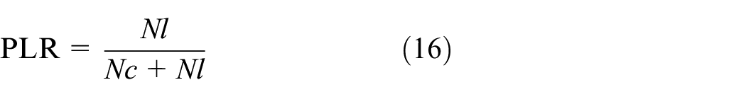
where Nc is the number of packets successfully collected and transmitted, and Nl is the number of packets unsuccessfully collected or transmitted.

Time-delay (t) refers to the time required for the network to successfully collect and transmit a data packet to the sink node. It is the sum of transmission delay (t_t), propagation delay (t_p), processing delay (t_pr), and queuing delay (t_q), that is

t = t_{t} + t_{p} + t_{pr} + t_{q}

(17)

Assuming that the size of each data packet collected is equal to lp (bit), and the queuing delay is negligible. Thus

\begin{matrix} t = (N_{r} + 1) (τ_{t} + τ_{pr}) + t_{p} = (N_{r} + 1) (\frac{lp}{R_{b}} + τ_{pr}) \\ + \sum_{k = 0}^{N_{r} - 1} \frac{d_{k (k + 1)}}{0.75 c} \end{matrix}

(18)

where N_r is the number of relay nodes. The 0th relay node is the source node, and the (N_r + 1)th relay node is the sink node. τ_t and τ_pr denote the transmission delay and the processing delay of the node to send a single data packet, respectively. d_k_(k + 1) is the Euclidean distance between the kth relay node and the (k + 1)th relay node. It should be mentioned that the propagation speed of light is approximately equal to 0.75c because of the underwater environment.

The average time-delay is defined as the ratio of the total delay (T = Σt) to the number of packets collected (Nc) during the lifetime of networks.

Algorithm description

The proposed algorithm can be divided into four main stages: deployment, redeployment, data collection, and data transmission.

Deployment and redeployment approach

3D network topology of underwater optical sensor network is depicted in Figure 3. Beneath the water surface, nodes transmit data through optical links with other nodes, AUV³⁰ (autonomous underwater vehicle) or submarine, and surface gateway nodes. The data transmission between nodes is mostly from bottom to top, and finally, to the surface gateway nodes for the sake of convenient and safe data storage and processing.³¹ Over the water surface, surface gateway nodes can directly or indirectly communicate with buoys, ships, ground stations, satellites, and so on, via radio (including radio frequency links and satellite communication links).

Figure 3.

3D network topology of underwater optical sensor network.

The underwater nodes are divided into static nodes and movable nodes. After filling the monitoring space with rhombic dodecahedrons, static nodes are anchored at the center of each rhombic dodecahedron for long-term monitoring. The movable nodes are randomly placed on the water surface. This process is called deployment.

In order to simplify the analysis, it is assumed that the gravity and buoyancy received by movable nodes are the same in size and the opposite in direction. The movable nodes adjust their depths on the basis of their exerted virtual force and move with the change of the area-of-interest. This process is called redeployment.

Besides different mobility of the two types of nodes, the rest of the functions and parameter setting are homogeneous, including as follows:

Data collection with sensing radius r_s (types of data include environmental parameters such as pressure and temperature, and services such as voices, images, and videos).

Data transmission with communication radius r_c.

Data storage, processing, and computing.

Initial energy E₀.

The movement of movable nodes consumes energy E_m

E_{m} = e_{m} \times | l |

(19)

where e_m is the energy consumption for moving per unit distance, and |l| is the moving distance.

Algorithm 1 is the pseudocode of the detailed process redeployment.

Algorithm 1. Redeployment algorithm.
Input: The number of static nodes N_s and movable nodes N_m, and their IDs n₁∼n_Ns, n_Ns₊₁∼n_Ns_+m, their original coordinates as well as their original residual energies. Preinstall threshold d_th and communication radius r_c; Output: The coordinates and residual energies of movable nodes;
1:	for i = 1:(N_s+N_m) do
2:	forj = 1:(N_s+N_m) do
3:	Compute the Euclidean distance between n_i and n_j;
4:	ifd_ij ≤ r_c then
5:	n_i obtains and stores the ID and coordinate of n_j;
6:	Compute $F_{ij}^{'}$ using equations (8)–(11);
7:	end if
8:	end for
9:	Compute F _{b i} using equation (12), then
10:	Compute l_i using equations (13) and (14);
11:	ifi > N_s then
12:	z_i ← z_i+ l_i ;
13:	Compute E_m(i) using equation (19);
14:	E_i ← E_i − E_m(i);
15:	end if
16:	end for

It should be noticed that Line_5 shows the process of information exchange between neighbor nodes: each node broadcasts a “Hello” message that includes its ID and coordinate. At the same time, each node receives its neighbors’“Hello” messages, and then calculates the distance between them, and adds this distance and neighbors’ IDs and coordinates into its storage. This process follows the Request To Send/Clear To Send (RTS/CTS) handshake protocol in medium access control (MAC) layer.³²

After the redeployment, the network coverage ratio C is calculated. It is defined as the ratio of the space that can be monitored by all nodes to the total monitoring area

C = \frac{⋃_{i = 1}^{N} V_{n} (i)}{V}

(20)

where V is the total volume of the monitoring area that is usually set as a rectangular space. V_n(i) is the volume of the area that can be monitored by the node n_i. Assuming that the nodes are equipped with omnidirectional antennas, so their monitoring area is a sphere area with the node as the sphere center and r_s as the radius.

If the coverage of the network is not convergent after adjustment, the next redeployment process continues. After the coverage ratio is converged (the numerical difference in coverage ratio between before-adjusted and after-adjusted network is less than or equal to 0.2%), the movable node will stay stable and the network starts to collect and transmit data.

Data collection and transmission

Only the data collection and transmission under the water is considered in this article. It is supposed that data randomly appears in the monitoring space, which will be collected by the nearest node. After simple processing and calculation, the data are transmitted from the bottom to the surface gateway node based on VBF protocol.

Algorithm 2 is the pseudocode of the detailed process of data collection and transmission.

Algorithm 2. Data collection and transmission algorithm.
Input: The number of both kinds of nodes N, their ID and coordinates, and their original residual energies E₁∼E_N. Sensing radius r_s and communication radius r_c, the minimum residual energy required for a node to work properly E_min. The acceptable maximum lost packets Nl_th, and the maximum amount of non-working nodes N_nwth within the lifetime. Output: The nodes’ updated residual energies. The number of collected packets Nc, and the number of lost packets Nl, the total time-delay T.
1:	Initiate Nl ← 0; Nc ← 0; T ← 0;
2:	while Nl < Nl_th do
3:	N_nw ← 0;
4:	fori = 1:N do
5:	ifE_i < E_minthen
6:	N_nw ← N_nw + 1;
7:	end if
8:	end for
9:	ifN_nw > N_nwth then
10:	break;
11:	end if
12:	Randomly generate a data packet within monitoring area;
13:	Find the closest node n_{ID_co} to packet with distance d_min;
14:	ifd_min > r_s\|\| E_{ID_co} ≤ E_minthen
15:	Nl ← Nl + 1;
16:	continue;
17:	end if
18:	Compute E_t(ID_co) using equations (4), (6), and (7), where d ← 2 × d_min;
19:	E_{ID_CO} ← E_{ID_CO}-E_t(ID_co);
20:	ID_tr ← ID_co;
21:	whilez_{ID_tr} < 0 do
22:	forj = 1:N do
23:	if $j \neq I D_{-} tr$ &&d_{jID_tr}&&z_j > z_{ID_tr} then
24:	Compute μ(ID_tr, j) using equation (15);
25:	elseμ(ID_tr, j) ← 0;
26:	end if
27:	ifμ is empty then
28:	Nl ← Nl + 1; Compute t using equation (18); T = T + t;
29:	break;
30:	else Find the node n_{id_tr} minimizing μ(ID_tr, id_tr);
31:	end if
32:	ifE_{ID_tr} ≤ E_minthen
33:	Nl ← Nl + 1; Compute t using equation (19); T = T + t;
34:	break;
35:	else Compute E_t(ID_tr); E_{ID_CO} ← E_{ID_CO}-E_t(ID_co);
36:	ID_tr ← id_tr;
37:	end if
38:	end while
39:	Nc ← Nc + 1; Compute t using equation (19); T = T + t;
40:	end while

First, check whether the lifetime ends. When too many packets are lost or too many nodes stop working, the network’s lifetime ends (Lines_2∼11). Next, the data packets will be collected (Lines_12∼20). But if the data packets appear outside the coverage of the network or the residual energy of the collecting node is not enough, the data packet will lose (Lines_14∼17). It should be noted that the signal for data collection is sent and received by the same sensor, so the distance of optical transmission is twice the distance from the node to the location of the packet (Line_18). After the data being successfully collected, data transmission will be performed according to the VBF protocol (Lines_21∼38). If there is no upper-level neighbor node (Lines_27∼29) or the residual energy of relay node is not enough (Lines_32∼34) during the transmission process, the packet-loss happens.

Simulation results and discussion

As a calculation example, the monitoring area is set to a cube area of 200 m × 200 m × 200 m. Specific parameter settings are shown in Table 1. The performance of RBDA is evaluated in five aspects: coverage ratio, lifetime, residual energy variance, PLR, and average time-delay, which are also compared with several existing classic deployment methods.^18,19,21

Table 1.

Parameter setting.

Parameter	Value
r_s	20 m
r_c	40 m
N_s:Nm	1:1
E ₀	50 J
e_m	1 mJ
E _min	1 J
l _max	10 m
φ, θ	60°, 5°
A_r	0.01 m
η_t, η_r	0.9, 0.9
η _PD	0.85
R_b	5 Mbps
λ	520 nm
k(λ)	0.2
K_r, K_a	60, 0.5
K_b	1.5
d_th	31.78 m
d_bth	20 m
τ_pr	0.2 s
lp	4 Mbit
к	0.1

Coverage ratio

The virtual force model is introduced to increase network coverage ratio. A total of 200 nodes (100 static nodes and 100 movable nodes) are deployed in the monitoring area. The network coverage ratio of different algorithms during the redeployment process with the number of iterations is shown in Figure 4.

Figure 4.

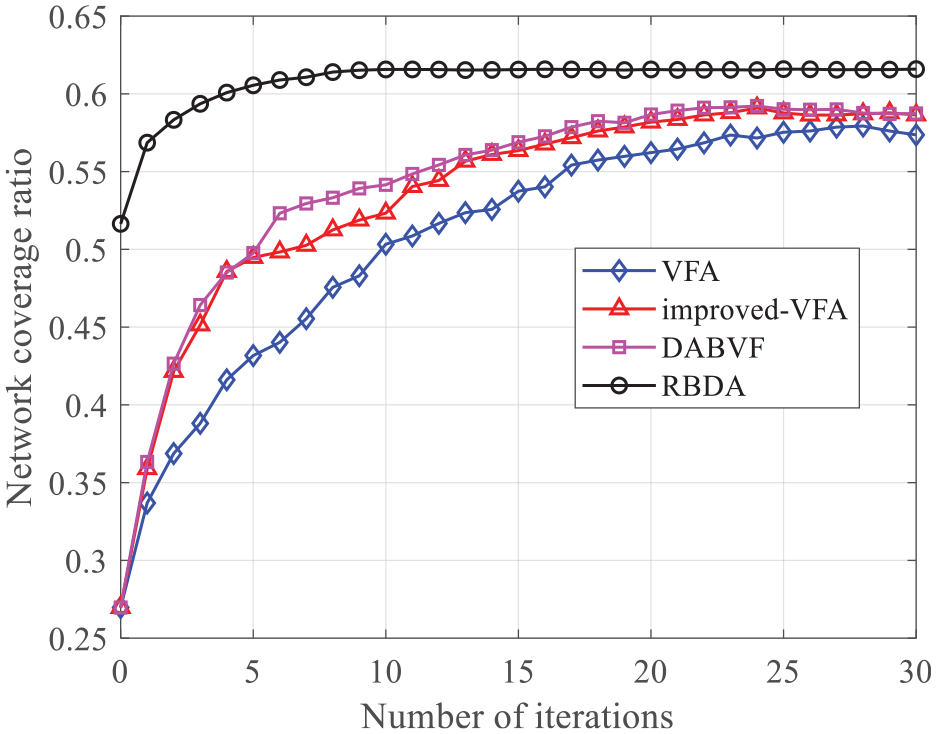
Network coverage ratio versus the number of iterations.

RBDA is significantly better than other algorithms in terms of coverage ratio, as well as the rate of convergence. The coverage ratios of the four algorithms when having been converged are 57.35% for virtual force algorithm (VFA), 58.18% for improved-VFA, 58.24% for distributed node deployment algorithm based on virtual force (DABVF), and 60.89% for RBDA, respectively. Besides, the numbers of iterations are 23 times for VFA, 20 times for improved-VFA, 18 times for DABVF, and only 7 times for RBDA when the coverage ratio of the network is converged. In this case, the RBDA can achieve the same coverage ratio as the purely dynamic deployment method with fewer nodes, and therefore, it is more cost-effective.

Lifetime and residual energy variance

The number of data packets collected within normally working state of the network is called lifetime, measuring the utilization rate of network energy. After the network stops working (lifetime ends), the variance of the residual energy of all nodes is calculated, which measures the balance of energy consumption of the network.³³

Figure 5 shows the lifetime of different algorithms with the initial number of nodes obtained by simulation. In the early deployment process of the RBDA, the moving distance of the nodes is shorter, the energy consumption is lower, and the coverage rate of the network is higher, so the lifetime of RBDA nearly doubles the other algorithms.

Figure 5.

Network lifetime versus the number of nodes.

Figure 6 shows the variance of the residual energy of different algorithms with the number of nodes. In general, the residual energy variance decreases with the number of nodes. RBDA and DABVF both introduce mobile benefit coefficient, so the residual energy variances are much lower than the other two algorithms, indicating that network energy consumptions of these two algorithms are more balanced.

Figure 6.

Residual energy variance versus the number of nodes.

Package-loss rate and average time-delay

The PLR and the time-delay are typical network routing performances. The routing performances between the RBDA and several existing deployment algorithms are simulated and compared using the same VBF protocol.

The PLRs of different algorithms with the number of nodes are shown in Figure 7. It can be seen that the PLR of RBDA is much lower than (nearly half of) the other three algorithms when the number of initial nodes is the same.

Figure 7.

Packet-loss rate versus the number of nodes.

The average time-delay of different algorithms with the number of nodes is shown in Figure 8. It can be seen that the average time-delay gradually decreases with the number of nodes. In the case of the same number of nodes, the RBDA has the lowest average packet-delay.

Figure 8.

Average time-delay versus the number of nodes.

From Figures 4 –8, regarding the common criteria of the deployment algorithms, RBDA can achieve a higher and more fast-converged coverage ratio of networks, a longer lifetime, and a more balanced energy consumption. Besides, RBDA is a routing-benefited deployment algorithm, as two important performances of routing, namely, package-loss rate and time-delay, can be greatly improved by RBDA.

Conclusion

Network deployment is important for efficient networking and reliable communication. We proposed RBDA for the underwater wireless optical sensor network using the virtual force model and VBF protocol. Also, RBDA is compared with relevant algorithms. The numerical results show that it outperforms in coverage, energy, and routing performances.

In the future, more environmental factors should be considered in the deployments, such as water currents and vortices. Localization algorithms and transmitting protocols combined with specific deployment approaches also have research value. Besides, research works for underwater wireless optical communication technologies should be more in-depth to further accelerate the practical application.

Footnotes

Handling Editor: Yanjiao Chen

Declaration of conflicting interests

The author(s) declared no potential conflicts of interest with respect to the research, authorship, and/or publication of this article.

Funding

The author(s) disclosed receipt of the following financial support for the research, authorship, and/or publication of this article: This work was supported by the National Natural Science Foundation of China (NSFC) under grant nos 61871418 and 61801079, China.

ORCID iD

Hongxi Yin

References

Xing

Yin

, et al. Joint relay selection and power allocation for underwater cooperative optical wireless networks. IEEE T Wirel Commun 2020; 19: 251–264.

Elamassie

Miramirkhani

Uysal

Performance characterization of underwater visible light communication. IEEE T Commun 2019; 67: 543–552.

Gao

, et al. A constant factor approximation for the d-hop connected dominating set in three-dimensional wireless networks. IEEE T Wirel Commun 2019; 18: 4357–4367.

Felemban

Shaikh

Qureshi

, et al. Underwater sensor network applications: a comprehensive survey. Int J Distrib Sens N 2015; 11: 1–14.

Wang

Lin

Yang

, et al. An energy-efficient compressive sensing-based clustering routing protocol for WSNs. IEEE Sens J 2019; 19: 3950–3960.

Jouhari

Ibrahimi

Tembine

, et al. Underwater wireless sensor networks: a survey on enabling technologies, localization protocols, and internet of underwater things. IEEE Access 2019; 7: 96879–96899.

Garcia

Sendra

Atenas

, et al. Underwater wireless ad-hoc networks: a survey. In: Loo

Mauri

Ortiz

(eds) Mobile ad hoc networks: current status and future trends. 1st ed. Boca Raton, FL: CRC Press, 2012, pp.379–411.

Tuna

Gungor

VC.

A survey on deployment techniques, localization algorithms, and research challenges for underwater acoustic sensor networks. Int J Commun Syst 2017; 30: e3350.

Wang

Shen

Shi

, et al. A novel energy-efficient contention-based MAC protocol used for OA-UWSN. Sensors 2019; 19: 183–196.

10.

Climent

Sanchez

Capella

, et al. Underwater acoustic wireless sensor networks: advances and future trends in physical, MAC and routing layers. Sensors 2014; 14: 795–833.

11.

Zeng

Zhang

, et al. A survey of underwater optical wireless communications. IEEE Commun Surv Tut 2017; 19: 204–238.

12.

Zhou

Yin

Yao

Wireless optical communication performance simulation and full-duplex communication experimental system with different seawater environment. In: Proceedings of the 2019 IEEE international conference on signal processing, communications and computing (ICSPCC’2019), Dalian, China, 20–23 September 2019, pp.1–4. New York: IEEE.

13.

Kaushal

Kaddoum

Underwater optical wireless communication. IEEE Access 2016; 4: 1518–1547.

14.

Alam

SMN

Haas

. Coverage and connectivity in three-dimensional networks. In: Proceedings of the 12th annual international conference on mobile computing and networking (MobiCom’06), Los Angeles, CA, 23–26 September 2006, pp.346–357. New York: ACM Press.

15.

Alam

SMN

Haas

. Topology control and network lifetime in three-dimensional wireless sensor networks. arXiv Computer Science, https://arxiv.org/abs/cs/0609047 (2006, accessed 27 October 2020).

16.

Liu

A deployment algorithm for underwater sensor networks in ocean environment. J Circuit Syst Comp 2011; 20: 1051–1066.

17.

Jiang

Wang

Liu

A sensor redeployment algorithm based on virtual forces for underwater sensor networks. Chinese J Electron 2018; 27: 413–421.

18.

Zou

Chakrabarty

. Sensor deployment and target localization based on virtual forces. In: Proceedings of the 22nd annual joint conference of the IEEE computer and communications societies (IEEE INFOCOM 2003), San Francisco, CA, 30 March–3 April 2003, pp.1293–1303. New York: IEEE.

19.

Yang

, et al. Deploying three-dimensional mobile sensor networks based on virtual forces algorithm. In: Proceedings of the China conference on wireless sensor networks (CWSN’2012), Huangshan, China, 25–27 October 2012, pp.204–216. Berlin: Springer.

20.

Boufares

Khoufi

Minet

, et al. Three dimensional mobile wireless sensor networks redeployment based on virtual forces. In: Proceedings of the 2015 international wireless communications and mobile computing conference (IWCMC), Dubrovnik, 24–28 August 2015, pp.563–568. New York: IEEE.

21.

Liu

Zhao

, et al. A distributed node deployment algorithm for underwater wireless sensor networks based on virtual forces. J Syst Architect 2019; 97: 9–19.

22.

Xing

Yin

, et al. An adaptive and energy-efficient algorithm for surface gateway deployment in underwater optical/acoustic hybrid sensor networks. IEEE Commun Lett 2018; 22: 1810–1813.

23.

Wang

Shi

, et al. Design of optical-acoustic hybrid underwater wireless sensor network. J Netw Comput Appl 2017; 92: 59–67.

24.

Yadav

Kumar

Optimal clustering in underwater wireless sensor networks: acoustic, EM and FSO communication compliant technique. IEEE Access 2017; 5: 12761–12776.

25.

Xing

Yin

Shen

, et al. Joint relay assignment and power allocation for multiuser multirelay networks over underwater wireless optical channels. IEEE Internet Things 2020; 7: 9688–9701.

26.

Nguyen

Mai

VV.

Underwater optical wireless communication-based IoUT networks: MAC performance analysis and improvement. Opt Switch Netw 2020; 37: 100570.

27.

Giles

Bankman

IN.

Underwater optical communications systems. Part 2: basic design considerations. In: Proceedings of the 2005 IEEE military communications conference (MILCOM 2005), Atlantic City, NJ, 17–20 October 2005, pp.1700–1705. New York: IEEE.

28.

Detweiler

Doniec

Vasilescu

, et al. Autonomous depth adjustment for underwater sensor networks. In: Proceedings of the 5th ACM international workshop on underwater networks (WUWNet 2010), Woods Hole, MA, 30 September–1 October 2010, pp.1–4. New York: ACM Press.

29.

Xie

Zhou

Nicolaou

, et al. Efficient vector-based forwarding for underwater sensor networks. EURASIP J Wirel Comm 2010; 2010: 195910.

30.

Kang

Aldwairi

Kim

KI.

A survey on network simulators in three-dimensional wireless ad hoc and sensor networks. Int J Distrib Sens N. Epub ahead of print 6 October 2016. DOI: 10.1177/1550147716664740.

31.

Vieira

LFM

. Underwater sensor networks. In: Loo

Mauri

Ortiz

(eds) Mobile ad hoc networks: current status and future trends. 1st ed. Boca Raton, FL: CRC Press, 2012, pp.413–424.

32.

Jiang

State-of-the-art medium access control (MAC) protocols for underwater acoustic networks: a survey based on a MAC reference model. IEEE Commun Surv Tut 2018; 20: 96–131.

33.

Lin

Min

An energy-saving routing integrated economic theory with compressive sensing to extend the lifespan of WSNs. IEEE Internet Things 2020; 7: 7636–7647.

A routing-benefited deployment approach combining static and dynamic layouts for underwater optical wireless networks

Abstract

Keywords

Introduction

Related work

Preliminaries

Underwater optical wireless communication model

3D virtual force model

Underwater sensor network routing

Algorithm description

Deployment and redeployment approach

Data collection and transmission

Simulation results and discussion

Coverage ratio

Lifetime and residual energy variance

Package-loss rate and average time-delay

Conclusion

Footnotes

Declaration of conflicting interests

Funding

ORCID iD

References