
Abstract
Blade icing problems are ubiquitous for wind turbines located in cold climate zones. Data-driven indirect icing detection methods based on supervisory control and data acquisition system have shown strong potential recently. However, the supervisory control and data acquisition data is annotated through manual observation, which will cause the data between normal condition and icing condition to be unlabeled. In addition, the amount of normal data is far more than icing data. The above two issues restrict the performance of most current data-driven models. In order to solve the label missing problem, this article proposes a Pearson correlation coefficient–based algorithm for measuring the degree of blade icing, which calculates the similarity between the unlabeled data and the icing data as its label. Aiming at the class-imbalance problem, this article constructs multiple class-balanced subsets from the original dataset by under-sampling the normal data. Temporal convolutional networks are trained to extract features and make predictions on each subset. The final prediction result is obtained by ensembling the prediction results of all temporal convolutional network models. The proposed model is validated using the actual supervisory control and data acquisition data collected from a wind farm in northern China, and the results indicate that ensuring the consecutiveness and class-balance of the data are quite advantageous for improving the detection accuracy.
Keywords
Introduction
With the depletion of global fossil energy and the trend of global warming, wind power, as one of the clean and renewable energy sources, has attracted much attention from countries around the world. Wind farms, where wind turbines (WTs) are installed to collect wind energy, are distributed across a wide range of climates, especially cold climates. 1 Cold climate areas are usually characterized by high altitude, low temperature, and high humidity, where WT blades are prone to icing. Blade icing will severely affect the power output of the WT as well as the life span of equipment, and even endanger personal safety. Therefore, it is of vital significance to realize WT blades icing detection in early stage and activate the de-icing system2,3 to remove ice. Recent icing detection methods can be divided into two categories: direct detection methods and indirect detection methods. Direct detection methods rely on additional sensors4–6 to detect physical properties changes in blades (such as emissivity, conductivity, and mass) to determine whether there is icing. However, most of the WTs in service do not have those direct detection sensors, and the installation of those sensors is complicated and expensive, so direct ice detection method is only feasible on a few of newly installed WTs.
On the contrary, with the popularization of supervisory control and data acquisition (SCADA) system in wind farms, data-driven icing detection methods have gradually become mainstream. 7 Indirect detection methods usually use machine learning techniques to reveal the inherent connection between data provided by the SCADA system and icing condition. These data include WT state data, environmental data, and WT motion data. Some researchers have established icing prediction models based on traditional machine learning methods.8–13 However, traditional machine learning models rely on feature engineering, which is time-consuming and labor-intensive. Besides, due to the restriction of model size, they often fail to make good use of temporal relationships between data. As an emerging branch of machine learning, deep learning has been widely used in fault diagnosis14–18 and achieves great success because of its outstanding ability to automatically extract effective features from big data. Among them, there is no lack of research in the field of WT icing detection. Liu et al. 19 found that the representative features automatically extracted by a deep autoencoder laid a foundation for detecting icing conditions. The authors also ensembled features from different hidden layers of the deep autoencoder model to improve detection accuracy. Yeh et al. 20 combined convolutional neural networks (CNN) and support vector machine to predict long cycle maintenance time of WTs. Yun et al. 21 established a well-behaved icing detection model using the SCADA data of one WT and applied the idea of transfer learning to make the model applicable to more WTs. As a specialist for time-series modeling, recurrent neural networks (RNN) have also been explored in WT fault detection.22,23 Benefiting from their strong feature extraction and big data processing capabilities, deep learning models have a prominent improvement in detection accuracy over traditional machine learning models.
Nevertheless, two key characteristics of the WT SCADA data that will affect the prediction accuracy are not taken into account by the above deep learning models. The first characteristic is that there exists some unlabeled data in the dataset. At present, the annotation of the dataset mainly relies on human labor. Staff in the wind farm observes the state of a WT at certain moments and record whether it is icing. The disadvantage of this approach is that when the staff first discovers the icing condition, he cannot determine whether the state of the WT between that moment and the last observed non-icing moment is icing or not. Therefore, some data is unlabeled. Since supervised learning requires each data to have a label, almost all present data-driven models only keep labeled data and ignore unlabeled data. There are some potential issues that arise from this practice. First, the dataset will be inconsecutive. Usually, the unlabeled data is between normal data and icing data. The performance of a time-series model will be largely affected by the consecutiveness of the dataset. Second, icing data is very precious in SCADA data. The unlabeled data contains important information related to icing conditions. Effective use of unlabeled data helps to better mine the features under icing conditions. The second characteristic of SCADA data is that it is class-imbalanced, which indicates that the amount of normal data is far more than that of icing data. The methods to tackle class-imbalance are divided into two categories: data preprocessing and algorithm optimization. Data preprocessing methods include under-sampling major class data, 24 over-sampling minor class data, 25 and generating minor class data. 26 Nevertheless, down-sampling will cause information loss. Over-sampling may give rise to over-fitting problems, and generating minor class data will inevitably introduce noise. Algorithm optimization methods attempt to modify the evaluation metrics and loss function, forcing them to pay more attention to minor class data. Chen et al. 27 noticed the class-imbalance problem in WT SCADA data and proposed a deep neural network based on triplet loss. However, the authors did not make full use of the unlabeled data. We summarize the merits and drawbacks of above-mentioned WT icing detection models based on deep learning techniques in Table 1.
Reviews on WT icing detection models based on deep learning techniques.

WT: wind turbine; CNN: convolutional neural network. LSTM: long short-term memory; TL-DNN: triplet loss deep neural network.
Handling the above two key characteristics of WT SCADA data is essential to establish an accurate icing detection model. To deal with unlabeled data, we present a Pearson correlation coefficient (PCC)-based algorithm for measuring the degree of blade icing. The degree of blade icing is regarded as the label of the unlabeled data. The SCADA data covers a long period of time, and some of the parameters in it are sensitive to time due to factors such as weather and control strategies. Thus, when measuring the degree of icing of the unlabeled data in a certain period of time (i.e. calculating the PCC), comparisons should be made locally instead of globally. Exponential moving average (EMA) is introduced to process normal data and icing data within a period of time before and after unlabeled data as the comparison standard. We call these data labeled by this algorithm soft-labeled data. Aiming at the class-imbalanced problem, we put forward an ensemble learning method that trains multiple models on multiple subsets and averages the prediction results of all models as the final prediction result. Our ensemble method is a bit different from the classic ensemble learning method-Bagging. Bagging obtains multiple subsets on the original dataset by means of sampling with replacement. The subsets may still suffer from class-imbalance problem. Our method just samples the normal data of the original dataset without replacement, and the soft-labeled data along with the icing data are all allocated to each subset, so each subset is class-balanced. The prediction model chosen in this article is temporal convolutional network (TCN). The advantages of RNN are that all historical inputs will be considered when calculating the output at the current moment, and there is a strict causal relationship between inputs and outputs. TCN takes the advantages of RNN to improve conventional CNN. Thus, TCN has a larger receptive field than conventional CNN under the same convolution kernel. In addition, TCN also guarantees the causality between inputs and outputs. We also use a mixed loss function that combines focal loss and mean square error (MSE) as the loss function. Since focal loss can only be used for classification problems, we use MSE to calculate the prediction error of those soft-labeled data. The final prediction result is obtained by averaging the prediction results of all TCN models trained on each subset. The contributions of this article are listed below:
Aiming at the label-missing problem in WT SCADA data, we propose a novel PCC-based algorithm. The algorithm measures the similarity between unlabeled data and adjacent labeled data to annotate unlabeled data. Thereby, the integrity of the dataset is guaranteed.
Aiming at the class-imbalance problem, we put forward an ensemble learning method. By evenly distributing the normal data in the original dataset to each subset and adding all icing data to each subset, multiple class-balanced subsets are constructed. The deep learning models are trained on these subsets, and the final prediction result is determined by averaging the results of all models.
Deep TCN and a mixed loss function are integrated as the icing detection model, in which the temporal and spatial features of the data are fully considered. The mixed loss function is composed of focal loss and MSE. Our model works directly on raw data and thus no feature extraction stage or extra domain knowledge is required.
The rest of this article is organized as follows. Section “Proposed model” describes the proposed model in detail. Section “Experiment preparation” introduces the method of data preprocessing and model evaluation metrics. Section “Results analysis” analyzes the experiment results and section “Conclusion” summarizes the work in this article.
Proposed model
Figure 1 describes the whole structure of our WT icing detection model. We first divide the original SCADA data into a training set and a testing set. In the training set, the PCC-based algorithm for measuring the degree of WT blade icing is used to annotate the unlabeled data. Originally, label 0 indicates that the WT is in normal condition, and label 1 indicates that the WT is in icing condition. This is a typical two-class classification problem. Considering that WT blade icing is a gradual process, the condition of the WT corresponding to the unlabeled data is between the normal condition and the icing condition, which can be regarded as a transition state. Specifically, we quantify this condition and use PCC between the unlabeled data and the icing data to measure the degree of blade icing. As mentioned above, some parameters in the SCADA data change greatly over time, so the comparison is performed in a local period of time. For a certain segment of unlabeled data, we selected 60 data points before it and 60 data points after it as the comparison standard. EMA is used to calculate the moving average of normal data and icing data, respectively. After that, we calculate the PCC between the average normal data and the unlabeled data, and the PCC between the average icing data and the unlabeled data. The two PCC values are processed with softmax function. Finally, we choose the PCC between the unlabeled data and the average icing data after softmax processing as its label. If the label is close to 1, the correlation between the two data is very high, indicating that the icing condition severe; if the label is close to 0, the correlation is low, indicating that the WT is in normal condition. The algorithm is also applied in the testing set. However, in order to ensure the correctness, the prediction results of these soft-labeled data are not included in the calculation of the evaluation metrics. Adding these data is mainly to maintain the consecutiveness of the dataset to improve the prediction results. Correspondingly, the output of the model during the training process becomes the degree of icing (a number between 0 and 1), and the output of the model during the testing process is still the classification result of whether it is icing. Afterward, we divide the normal data in the training set into eight equal parts due to the ratio of normal data to soft-labeled data together with icing data is about 8:1. Each subset contains all soft-labeled data, all icing data, and one part of normal data. Then we get eight class-balanced subsets. The icing detection model, TCN model, is trained on each subset. All eight TCN models have the same structure. Since they are trained on different subsets, their weights are different from each other. For a time-series data of length

The flowchart of our proposed WT icing detection model.

The TCN model utilized in our method.
PCC-based algorithm for measuring the degree of blade icing
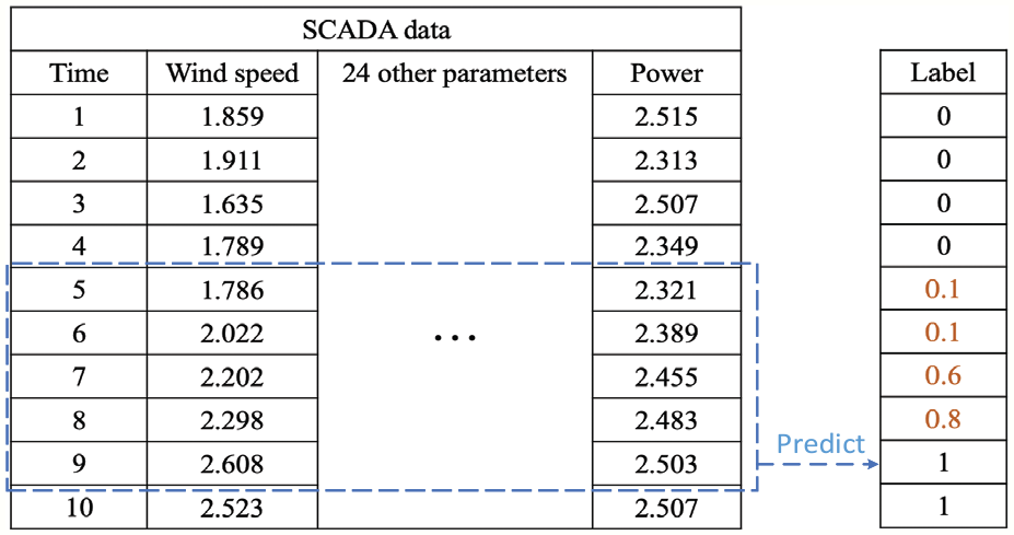
Figure 3 shows the data recorded by the SCADA system of a wind turbine in northern China. Each data point contains 26 parameters, such as wind speed and power. The detailed information of 26 parameters is listed in Table 2. The sampling interval of all parameters is the same, which is 10 s. The whole dataset is arranged in chronological order. The staff of the wind farm confirmed the condition of the WT every once in a while. For example, he found that the WT blades were normal at

An illustration for the reason why some data is unlabeled.
Parameters in SCADA data.

Nearly all present data-driven icing detection models ignore these unlabeled data, since only labeled data can be used to train the model according to the requirement of supervised learning. For conventional modeling problems, deleting part of the data has no effect, but WT icing detection is a time-series modeling problem. In other words, the output at the current moment is not only related to the input at the current moment but also related to the inputs at previous moments. For example, if we want to predict icing condition at


Other data-driven models deal with unlabeled data by ignoring it.
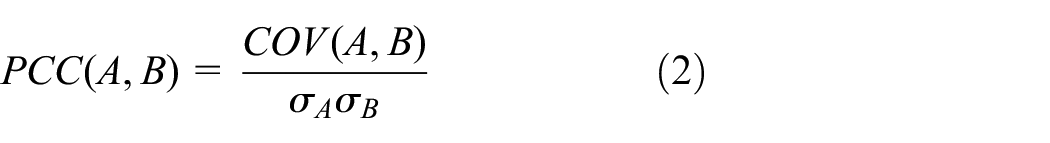
where
PCC-based algorithm for measuring the degree of blade icing.
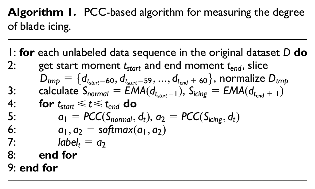
It can be seen that the label calculated by the above algorithm is a value between 0 and 1, which means that we have transformed the icing detection problem from a classification problem into a regression problem. The final output of the model is not a class (icing or normal), but a probability. Assuming that the WT is still in a normal state at
Our solution to unlabeled data.
The ensembling theory
The main idea of ensemble learning is to complete learning tasks by constructing and combining multiple models. Sometimes a single model may not be able to learn all the features from the data. Then we can build multiple models, each of which learns a part of features from the data, and ensemble the results of all models. This article adopts this method to cope with class-imbalance problem. In the original dataset, normal data accounts for the majority. If the under-sampling method is applied, a large amount of normal data will be discarded, resulting in the loss of useful information. If over-sampling icing data or generating icing data is used, it is difficult to determine where these newly generated data is placed in order to retain the temporal relationship of the original dataset. Our solution to preserve the integrity of the dataset and the temporal relationship between data is constructing eight class-balanced subsets of the original dataset. The first step is to divide the normal data into eight subsets, through random sampling without replacement. The second step is to add all soft-labeled data and icing data to each subset. In each subset, all data is arranged in chronological order to restore the temporal relationship. In the training process, models are trained on subsets respectively, so there is no ensembling step. In the testing process, the testing data is inputted into eight models to obtain eight prediction results (a number between 0 and 1) and then these results are averaged and rounded to get the final classification result.
Temporal convolutional network
TCN is a specially designed CNN for processing time-series data. Conventional CNN usually considers the spatial relationship of data other than temporal relationship, but time-series modeling needs to consider the temporal relationship. For example, only currently observed data (i.e. not future data) can be used to judge whether there is icing at the current time in our problem. Hence, some restrictions need to be added to the convolution operation to ensure this. For a time-series input of length
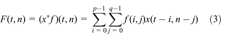
Since


Masked dilated convolution.
The main advantage of deep learning is that deeper networks can extract more intrinsic features, while too deep networks will lead to degradation problem. Residual block is able to ensure deeper layers contain more features than previous layers by introducing identity mapping. A residual block is calculated by the following equation

where
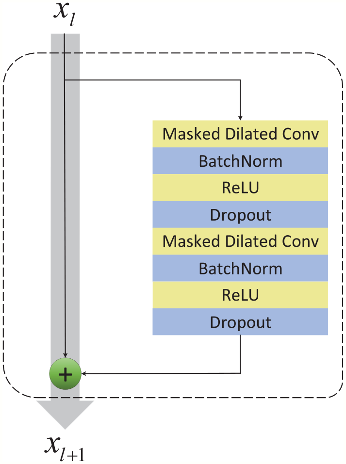
Residual block.
As mentioned in section “PCC-based algorithm for measuring the degree of blade icing,” the input of a time-series model is usually a data segment. We specify how the raw data is fed into TCN via sliding window method and how the output is concatenated, taking Figure 8 as an example. In the figure, the value of window length

An illustration of how the original data is sliced into data segments and fed into TCN.
For TCN, its receptive field should be larger than window length

Dilation factor
Our mixed loss function is expressed as follows

where
Experiment preparation
Data preprocessing
SCADA system records 26 parameters including motion parameters (such as angle of three blades and generator speed), state parameters (such as motor temperature of three blades, nacelle acceleration in X and Y direction, and nacelle temperature), and environmental parameters (such as wind speed, wind direction, and environment temperature). The abbreviation and physical meaning of all parameters are listed in Table 2. Although the importance of the 26 parameters for detecting icing conditions may be different, deep learning model can automatically learn useful features from the parameters. Therefore, this article uses all the parameters as the input of the model, instead of selecting only some of the parameters like some traditional machine learning models. 70% of the data is chosen as the training set and the rest 30% is chosen as the testing set. Researches8,12 have confirmed that analyzing wind speed-power curve is beneficial for icing detection. For example, when

Wind speed-power curve.
The value of parameters differs from each other, and we have to normalize them by the equation below

where
Model evaluation index
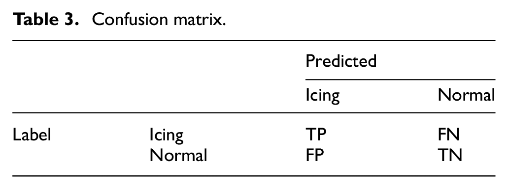
For class-imbalanced datasets, it is not comprehensive to evaluate a model only by accuracy, because the model can achieve high accuracy as long as all samples are classified as the major class. The confusion matrix and a series of evaluation metrics calculated by it are considered more objective to evaluate the performance of a model on class-imbalanced datasets. The confusion matrix is given in Table 3. TP represents the number of actual icing samples predicted to be icing samples; TN represents the number of actual normal samples predicted to be normal samples; FP represents the number of actual normal samples predicted to be icing samples; FN represents the number of actual icing samples predicted to be normal samples. Based on the confusion matrix, precision


Confusion matrix.

Results analysis
Our experiments are implemented on a Dell server with Intel E5-2620 CPU, 16G memory and two NVIDIA GTX1080 graphics cards. The programming language is Python and the deep learning framework is Keras (with Tensorflow backend). In section “Ablation experiment,” we design three comparative models. For the first model, we do not use PCC-based algorithm and do not use ensemble learning method. For the second model, we use PCC-based algorithm and do not use ensemble learning method. For the third model, we do not use PCC algorithm and use ensemble learning method. Through the experiments between our proposed model and the above comparative models, it is found that both PCC-based algorithm and ensemble learning method are effective in improving the detection accuracy. Then, we compare the proposed model with a variety of existing data-driven WT icing detection models, and the results are shown in section “PCC-Ensemble-TCN model versus other data-driven models.”
Ablation experiment
As mentioned above, three comparative models are established. For the first comparison model, the original dataset is not processed by the PCC-based algorithm, and the data without label will be discarded. The solution to class-imbalance problem is to downsample the number of normal data to the number of icing data. The structure of TCN remains the same. We call this model TCN model. For the second comparison model, the original dataset is processed by the PCC-based algorithm, so the unlabeled data is annotated. The solution to class-imbalance problem is to downsample the number of normal data to the sum of the number of icing data and the number of soft-labeled data. This model is referred to as PCC-TCN model. For the third comparison model, the original dataset is not processed by the PCC-based algorithm, and the data without label will be discarded. The ensemble learning method is adopted, which means that the original dataset is divided into multiple class-balanced subsets, and TCN models are trained on each subset. The final prediction results are acquired by ensembling the prediction result of each TCN model. We call this model ensemble-TCN model. Figure 10 shows a schematic diagram of the three comparison models. The hyperparameters of the TCN model are optimized by grid searching. Concretely, window length

Three comparative models: TCN model, PCC-TCN model, and Ensemble-TCN model.
The performance of four models is listed in Table 4. Comparing TCN model and PCC-TCN model, it can be found that the introduction of the PCC-based algorithm significantly improves the
Ablation experiment results.
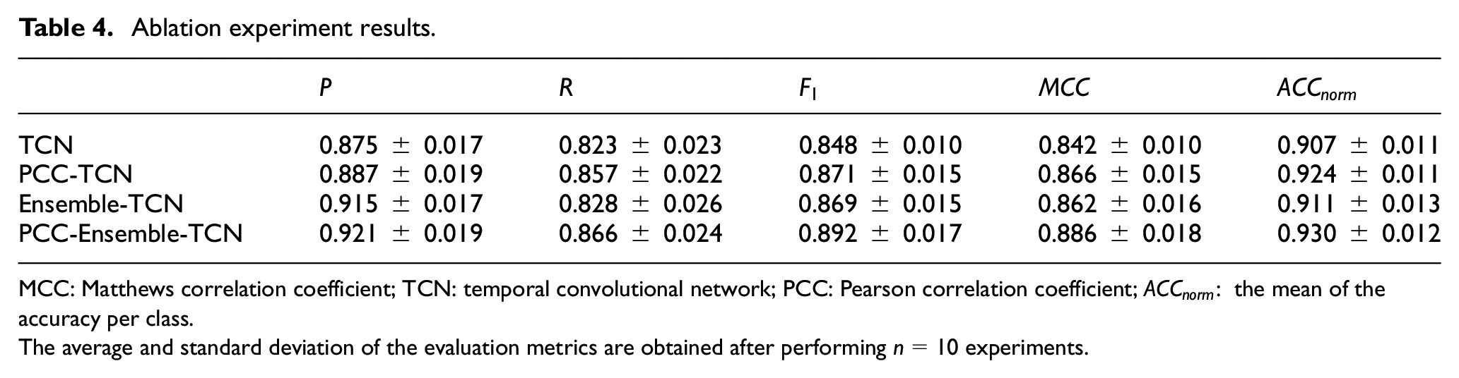
MCC: Matthews correlation coefficient; TCN: temporal convolutional network; PCC: Pearson correlation coefficient;
The average and standard deviation of the evaluation metrics are obtained after performing
Figure 11 shows a segment of the original dataset, where there is an obvious label missing problem. The original dataset consists of many such segments. The data for about 2 h from

An illustration of the label missing problem.
Using an autoencoder to annotate unlabeled data is an alternative method and may also achieve good effect as our PCC-based algorithm. Autoencoder is one of deep learning methods, which requires a lot of data for training. Whether in the training phase or the inference phase, the amount of calculation of autoencoder is much greater than our PCC-based algorithm. In addition, as a black box model, autoencoder is not as interpretable as our PCC-based algorithm. Unsupervised learning is also a promising technique. The SCADA data used in this article contains plenty of labeled data, and the non-supervised learning method does not make full use of these label information. For the above considerations, we prefer the PCC-based algorithm in this icing detection problem.
PCC-Ensemble-TCN model versus other data-driven models
We list some existing data-driven WT blades ice detection models and their performance in Table 5. Traditional machine learning model like particle swarm optimization-support vector machine (PSO-SVM) need to manually select features from many parameters, which is labor-intensive. In addition, it does not take full advantage of temporal relationship between data. In other words, PSO-SVM predicts whether there is icing condition only using the data at the current moment. It can be seen from the results that the
Performance of our proposed model and other data-driven models.
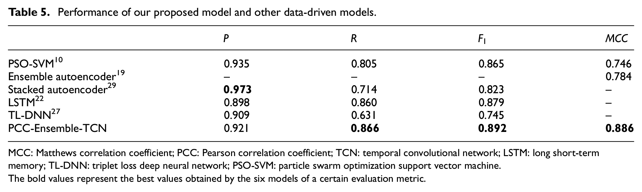
MCC: Matthews correlation coefficient; PCC: Pearson correlation coefficient; TCN: temporal convolutional network; LSTM: long short-term memory; TL-DNN: triplet loss deep neural network; PSO-SVM: particle swarm optimization support vector machine.
The bold values represent the best values obtained by the six models of a certain evaluation metric.
Conclusion
This article proposes a PCC-based algorithm for measuring the degree of blade icing and an ensemble learning model to deal with the label missing problem and the class-imbalance problem in the wind turbine SCADA data, which are neglected in recent data-driven models. The proposed PCC-based algorithm measures the similarity between the unlabeled data and nearby icing data as its label. This not only ensures the consecutiveness of the dataset but also replenishes the information under icing conditions. Afterward, we divide the normal data in the training set into eight equal parts due to the ratio of normal data to soft-labeled data together with icing data is about 8:1. Then eight class-balanced subsets are constructed. Each subset contains all soft-labeled data, icing data, and one part of normal data. The icing detection model, TCN model, is trained on each subset. In the TCN model, the original cross-entropy loss function is replaced with a mixed loss function that combines focal loss and MSE to focus on samples with large differences between the predicted results and the actual results (difficult-to-classify samples), thereby accelerating the convergence process of the model. We get the final prediction results by rounding the average values of eight prediction results acquired from eight TCN models. The proposed model is validated using the actual SCADA data collected from a wind farm in northern China, and the results indicate that ensuring the consecutiveness and class-balance of the data are quite advantageous for improving the detection accuracy by comparing with other data-driven models.
We present a time-series prediction model for anomaly detection, and this kind of problem can be found in many industrial scenarios.30–32 Since the model proposed in this article performs well in WT blades icing detection, it is conceivable that our proposed model should also be applicable to those problems, which needs to be further verified in the future.
Footnotes
Handling Editor: Francesc Pozo
Declaration of conflicting interests
The author(s) declared no potential conflicts of interest with respect to the research, authorship, and/or publication of this article.
Funding
The author(s) disclosed receipt of the following financial support for the research, authorship and/or publication of this article: This work was supported by the National Natural Science Foundation of China (Grants Nos. 11972115, 11572084).