A novel method for asynchronous source localisation based on time of arrival measurements

Abstract

Source localisation is an important component in the application of wireless sensor networks, and plays a key role in environmental monitoring, healthcare and battlefield surveillance and so on. In this article, the source localisation problem based on time-of-arrival measurements in asynchronous sensor networks is studied. Because of imperfect time synchronisation between the anchor nodes and the signal source node, the unknown parameter of start transmission time of signal source makes the localisation problem further sophisticated. The derived maximum-likelihood estimator cost function with multiple local minimum is non-linear and non-convex. A novel two-step method which can solve the global minimum is proposed. First, by leveraging dimensionality reduction, the maximum (minimum) distance maximum (minimum) time-of-arrival matching-based second-order Monte Carlo method is applied to find a rough initial position of the signal source with low computational complexity. Then, the rough initial position value is refined using trust region method to obtain the final positioning result. Comparative analysis with state-of-the-art semidefinite programming and min–max criterion-based algorithms are conducted. Simulations show that the proposed method is superior in terms of localisation accuracy and computational complexity, and can reach the optimality benchmark of Cramér–Rao Lower Bound even in high signal-to-noise ratio environments.

Introduction

In recent years, a lot of research has been done on wireless sensor networks (WSNs) and this technology has also been applied in many different fields ¹ which include battlefield surveillance, healthcare and environmental monitoring. Target localisation plays an essential role in these varieties of applications. In a distributed cooperative WSN, the unknown position of the source node can be obtained by measuring some characteristic features of the signal. ² The anchor nodes, which are sensors in the network with accurately known location, receive the signal transmitted by the source, and then send the measurement data to the data fusion centre (DFC). According to the received noisy data, the DFC gives an estimate of the location of source node.

Many measurement models can be used for source localisation including the time of arrival (TOA),^3,4 angle of arrival (AOA),^5,6 time-difference of arrival (TDOA),^7,8 received signal strength (RSS), ⁹ and a combination of these models.^10,11 Among the listed models, time information measurement based methods have the highest accuracy in localisation compared to RSS and AOA. TDOA model, however, involves a pre-process of pairwise subtraction causing a 3 dB increase in noise of the measurement data, ¹² which then results in a degradation in localisation accuracy. Therefore, this article focuses on the TOA-based localisation method.

In a TOA localisation approach, the signal’s time instant of arrival is measured. ¹³ Nonetheless, the main question is ‘how long the propagation time of the signal is?’ To know this, it is required that the anchor nodes exactly know the accurate start transmission time $t_0$ of the signal. In other words, the perfect clock synchronisation between the source and anchor nodes is required. However, synchronisation in most situations is not feasible because of the following reasons. First, the implementation of the synchronisation mechanism in a WSN is challenging. The complexity of the network increases with an increase in the accuracy requirement of the time synchronisation, and as such, results in a rapid raise in the economic cost of the network deployment. For an imperfect synchronisation WSN, it can be assumed that $t_0$ is approximately equal to zero. Specifically, it can be assumed that the variation range of $t_0$ is only tens of nanoseconds, which results in tens of metres of measurement error (e.g. assume $t_0~\mathcal{U}(10,40)$ nanoseconds as in Zou and Wan ¹⁴ ). Label $t_0$ in this case as ‘small $t_0$ ’. Second, in some special areas of use, for example, when there is an independent operating enemy flight target (source node) and the monitoring sensor system (anchor nodes) of a military surveillance zone, there are no possible means of actualizing synchronisation between them. In this case, $t_0$ can be considered as an arbitrary random number. This has an obvious physical meaning as the enemy target flight can enter the surveillance zone at any time without informing the monitoring sensors, that is, the source node can send a signal to the anchor nodes at an unknown arbitrary time $t_0$ . Without loss of generality, it can be assumed that $t_0~\mathcal{N}(0,4)$ , unit in seconds, which is just like in Xu et al. ¹⁵ Let $t_0$ in this case be represented as ‘arbitrary $t_0$ ’.

In this work, we concentrate on the source localisation problem in asynchronous networks, which means that it requires synchronisation among anchor nodes but not between the source node and the anchor nodes. Taking into account the relationship between the TOA measurement value and the actual distance value between the anchor nodes and the source node, it can be assumed that a bigger (smaller) TOA measurement value should correspond to a bigger (smaller) distance value. Then, the Monte Carlo (MC) method based on maximum (minimum) distance maximum (minimum) TOA matching (MDTM) is proposed to solve the asynchronous source localisation problem. With the proposed method, a rough initial position result can be obtained by very few computational resources. This rough positioning result provides a good initial iteration point for the subsequent trust region (TR) method, enabling it to converge to the true source position after only a few iterations.

The remaining contents are organised as follows. Section ‘Related work’ describes some of the latest research achievements in asynchronous source localisation. Section ‘Problem formulation’ describes the asynchronous source localisation problem formulation. In section ‘The proposed MDTM-based second-order MC method’, the MDTM-based second-order MC method is proposed to find a rough initial position of the signal source. Section ‘The TR refinement’ gives TR method used to refine the rough initial position. Numerical simulations are conducted in section ‘Numerical simulations’ to demonstrate the performance superiority of the proposed method. Finally, section ‘Conclusion’ summarises this article as well as proposes some future work.

Related work

As previously stated, inaccurate time synchronisation will result in a significant localisation error because electromagnetic waves travel at a very high speed. There are many ways to deal with the asynchronous TOA-based source localisation problem.

TDOA measurement model is a typical method used in asynchronous source localisation, which involves eliminating $t_0$ by pairwise subtraction. But on the other hand, TDOA method introduces a 3 dB increase in measurement data noise. Nevertheless, due to simplicity in implementation, the TDOA model has inspired many research works.^7,16,17 Another method for solving the problem is estimating the source position and signal transmission start time jointly by minimising the derived cost function. This can be done using semidefinite programming (SDP) ¹⁸ to find the minimum point of the error function. Related research works include Zou and Wan, ¹⁴ Xu et al. ¹⁵ and Vaghefi and Buehrer. ¹⁹ The min–max criterion-based algorithm (MMA) method in Xu et al. ¹⁵ and the method in Vaghefi and Buehrer ¹⁹ (labelled as ‘SDP 2013’) provide an adequate solution for the ‘small $t_0$ ’ case asynchronous positioning problem. But there are some decline in performance when solving the ‘arbitrary $t_0$ ’ case problem. And when the source node is outside the convex hull formed by the anchor nodes, SDP 2013 and method in Zou and Wan ¹⁴ (labelled as ‘SDP 2016’) give dissatisfactory positioning accuracy. Chen et al. ²⁰ proposed a proximal alternating minimisation positioning (PAMP) method, which divides the original asynchronous problem into two subproblems: the clock offset subproblem and the synchronous source localisation subproblem. PAMP has an excellent performance when coping with scenarios where the emitting sources are in or near the convex hull formed by the anchor nodes. However, the performance decreases sharply as the sources move far away from the convex hull. There are also many swarm intelligence metaheuristics ²¹ solving source localisation problem with satisfactory accuracy. However, they are usually used to deal with multi-sensor node cooperative localisation. Zhu et al. ²² proposed an improved MC method in an international conference earlier this year, which contains the preliminary idea of this article. A lot of extended work has been done in this work.

According to the literature survey above, two main problems with asynchronous localisation are the positioning accuracy when the source node is outside the convex hull formed by the anchor nodes and computational complexity in all typical and practical scenarios. In combining these issues, the study motivation is to enhance the positioning accuracy while maintaining a low computational complexity level.

Problem formulation

The TOA measurement model

Consider a WSN described in Figure 1 with $M$ distributed sensors (anchor nodes) with known coordinates ${\mathit{a}}_i=[x_i,y_i{]}^T(i=1,2,\dots ,M)$ , and a source node with unknown coordinates $\mathit{p}=[x,y{]}^T$ to be estimated. For the sake of simplicity, we only consider the target location in a two-dimensional plane, which can be easily extended to the three-dimensional case. For a line-of-sight (LOS) propagation environment, the TOA measured by the ith anchor node can be expressed as ¹⁵

$$t_i=\frac{1}{c}\Vert {\mathit{a}}_i-\mathit{p}{\Vert }_2+t_0+n_i,i=1,2,\dots ,M$$

(1)

where $c$ represents the propagation velocity of electromagnetic wave $(3\times {10}^8\mathrm{m}/\mathrm{s})$ , $\Vert ·{\Vert }_2$ represents the $l_2$ norm of the vector, $t_0$ is the unknown time instant at which the source transmits the signal to be measured, and $n_i~\mathcal{N}(0,{\sigma }_i^2)$ is the independent additive Gaussian white noise (AGWN) with zero-mean. Due to the unknown parameter $t_0$ , the anchor node can only measure the signal’s TOA $t_i$ , instead of the signal’s propagation time $\Vert {\mathit{a}}_i-\mathit{p}{\Vert }_2/c$ . To obtain signal propagation time, the source node must notify anchor node of the signal’s start transmission time $t_0$ in some way. Hence, this requires perfect clock synchronisation between the source node and the anchor nodes. In this asynchronous source location problem, the TOA measurements contain additional unknown parameters $t_0$ due to the lack of a perfect time synchronisation mechanism.

Figure 1.

A WSN with $M$ distributed sensors (anchor node) with known coordinates ${\mathit{a}}_i$ , and a source node with unknown coordinates $\mathit{p}=[x,y{]}^T$ to be estimated.

Problem modelling and transformation

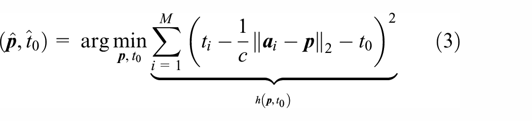
In an independent identically distributed Gaussian noise assumption $({\sigma }_i^2={\sigma }_t^2,i=1,2,\dots ,M)$ , the joint maximum-likelihood estimate (MLE) of $\mathit{p}$ and $t_0$ can be expressed as ²³

$$\begin{array}{c}\multicolumn{1}{c}{(\hat{\mathit{p}},{\hat{t}}_0)=\arg \underset{\mathit{p},t_0}{max}[{\left(\frac{1}{\sqrt{2\pi {\sigma }_t^2}}\right)}^M}\\ \times \exp (-\sum _{i=1}^M\frac{{(t_i-\frac{1}{c}{\Vert {\mathit{a}}_i-\mathit{p}\Vert }_2-t_0)}^2}{2{\sigma }_t^2})]\hfill \end{array}$$

(2)

The corresponding log-likelihood function (ignoring the constant term) is given by

$$(\hat{\mathit{p}},{\hat{t}}_0)=\arg \underset{\mathit{p},t_0}{min}\underset{h(\mathit{p},t_0)}{\underbrace{\sum _{i=1}^M{(t_i-\frac{1}{c}{\Vert {\mathit{a}}_i-\mathit{p}\Vert }_2-t_0)}^2}}$$

(3)

However, according to equation (1), the least-squares estimate of $t_0$ is

$${\hat{t}}_0=\frac{1}{M}\sum _{i=1}^M(t_i-\frac{1}{c}{\Vert {\mathit{a}}_i-\mathit{p}\Vert }_2)$$

(4)

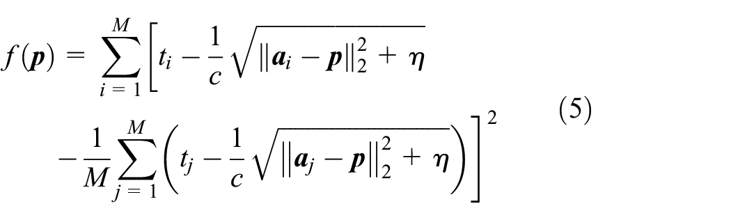
As Yao et al. ²⁴ proposed, we first use ${\hat{t}}_0$ to substitute $t_0$ in equation (3) and then by introducing a small constant $\eta$ , we get a differentiable objective function

$$\begin{array}{c}\multicolumn{1}{c}{f\left(\mathit{p}\right)=\sum _{i=1}^M[t_i-\frac{1}{c}\sqrt{\Vert {\mathit{a}}_i-\mathit{p}{\Vert }_2^2+\eta }}\\ {-\frac{1}{M}\sum _{j=1}^M(t_j-\frac{1}{c}\sqrt{\Vert {\mathit{a}}_j-\mathit{p}{\Vert }_2^2+\eta })]}^2\hfill \end{array}$$

(5)

Considering the differentiability of equation (5), now the TR method can be used to find the global minimiser of $f(\mathit{p})$ . To ensure the fast convergence of the TR method, one needs to provide a good initial iteration point. Hence, we propose the second-order MC method based on maximum (minimum) distance maximum (minimum) TOA matching (MDTM) to obtain rough initial positioning results, which provides a good initial iteration point for the TR method.

The proposed MDTM-based second-order MC method

This section focuses on describing the second-order MC method based on MDTM. MC method,^25,26 based on ‘randomness’ and the theory of probability and statistics, has been widely used as a very important numerical calculation method. The basic idea in using the MC method to solve the minimum point of an object function is to generate a large number of random points in the domain of the function, where each point represents a possible numerical solution. After the object function values at each point are calculated, the points with the smallest function value can be selected as the estimate of the minimiser of the object function. However, as the dimension of the problem increases, the large number of random points generated by the original MC method will consume huge computational resources.

To estimate the minimiser in a more computational cost saving way, we proposed the MDTM-based second-order MC method, which can reduce dimensionality when searching for solutions. Compared to the original MC method, this is a more effective way to obtain a relatively accurate solution, that is, a point that is exactly located within the basins of attraction which contains the true minimiser. The solution obtained by the second-order MC method based on MDTM provides a good initial iteration point for the subsequent TR method. The overall flow chart for solving asynchronous source location problems by the MDTM-based second-order MC method and TR method is described in Figure 2.

Figure 2.

The overall flow chart for solving asynchronous source localisation problem by the MDTM-based second-order MC method and TR method.

The first MDTM-based MC search

First, we describe the first MC search based on MDTM. The equivalent form of equation (3) is as follows

$$(\hat{\mathit{p}},{\hat{t}}_0)=\arg \underset{\mathit{p},t_0}{min}\underset{h_1(\mathit{p},t_0)=h_1\left(\mathbf{\theta }\right)}{\underbrace{\sum _{i=1}^M{[c(t_i-t_0)-{\Vert {\mathit{a}}_i-\mathit{p}\Vert }_2]}^2}}$$

(6)

where $\theta =[\mathit{p},t_0{]}^T$ is the problem variable. To estimate the minimiser point of $h_1(\mathbf{\theta })$ , we first uniformly and randomly generate $K_1$ of each of the first two dimensions of $\mathbf{\theta }$ according to the domain, that is, ${\mathbf{\theta }}_k(1,2)={\mathit{p}}_k=[x^{(k)},y^{(k)}{]}^T,k=1,2,\dots ,K_1$ . In order to balance positioning accuracy and computational efficiency, $K_1$ should not be too large. Note that each ${\mathbf{\theta }}_k$ represents a candidate for the estimate of the true minimiser of $h_1(\mathbf{\theta })$ .

Since the coordinates of anchor nodes are known, now the distances between each ${\mathit{p}}_k$ and each anchor node can be expressed as $d_i^k=\Vert {\mathit{a}}_i-{\mathit{p}}_k{\Vert }_2,i=1,2,\dots ,M$ . For each $k$ , let $d_{\max }^k$ denote the maximum distance, that is

$$d_{\max }^k=\underset{i=1,\dots ,M}{max}\Vert {\mathit{a}}_i-{\mathit{p}}_k{\Vert }_2$$

(7)

For a given set of TOA measurement values $t_i,i=1,2,\dots ,M$ , its maximum value is denoted as

$$t_{\max }=\underset{i=1,\dots ,M}{max}{t}_i$$

(8)

Ignoring the influence of measurement noise, it can be considered that the maximum $d_i^k$ matches with the maximum $t_i$ . This has an obvious physical meaning. When the source node sends signals to the anchor node at some fixed time instant $t_0$ , the farther the propagation distance (larger $d_i^k$ ) is, the longer the propagation time is, hence, the larger the signal’s TOA would be (larger $t_i$ ). Note that the minimum $d_i^k$ can also be selected to match the minimum $t_i$ .

Rearranging equation (1) we obtain

$$t_0=t_i-\frac{1}{c}\Vert {\mathit{a}}_i-\mathit{p}{\Vert }_2+n_i$$

(9)

In addition, considering the relationship between $d_{\max }^k$ and $t_{\max }$ and ignoring the noise term, an unbiased estimate of $t_0$ can be obtained by substituting $\Vert {\mathit{a}}_i-\mathit{p}{\Vert }_2$ and $t_i$ by $d_{\max }^k$ and $t_{\max }$ in equation (9), respectively, see equation (10a). Alternatively, the minimum $d_i^k$ and $t_i$ pairs can also be used to obtain the estimate of $t_0$ , see equation (10b)

$${\hat{t}}_0^k=t_{\max }-\frac{1}{c}{d}_{\max }^k,k=1,2,\dots ,K_1$$

(10a)

$${\hat{t}}_0^k=t_{\min }-\frac{1}{c}{d}_{\min }^k,k=1,2,\dots ,K_1$$

(10b)

Putting equations (10a) or (10b) into the third dimension of ${\mathbf{\theta }}_k$ , one get the MDTM-based MC random points ${\mathbf{\theta }}_k=[{\mathit{p}}_k^T,{\hat{t}}_0^k{]}^T=[x^{(k)},y^{(k)},{\hat{t}}_0^k{]}^T,k=1,2,\dots ,K_1$ in three-dimensional search space.

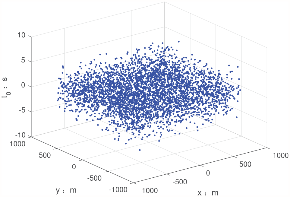
As an example in scenario 1 with ‘small $t_0$ ’ (which will be detailed in section ‘Numerical simulations’), Figures 3 and 4 show the distribution of random points generated by original MC method and the MDTM-based MC method, respectively. Note that the random points in Figure 3 are disordered and $t_0$ has a large variation range on the axis. Whereas in Figure 4, all random points are attached to a quasi-curved surface in three-dimensional space and $t_0$ has a small variation range on the axis. That is, the dimension of search space can be reduced by leveraging the inherent nature of MDTM, which greatly decreases the computational complexity. As equations (10a) and (10b) bring the same computational reduction effect, equation (10a) is selected as the third dimension of ${\mathbf{\theta }}_k$ in practice.

Figure 3.

The distribution of random points generated by original MC method.

Figure 4.

The distribution of random points generated by the proposed MDTM-based MC method (a) maximum distance maximum TOA matching and (b) minimum distance minimum TOA matching.

For each MC point ${\mathbf{\theta }}_k$ , first compute $h_1({\mathbf{\theta }}_k)$ . Then, select some $(\mathrm{Slt}\_\mathrm{num}\_1)$ of ${\mathbf{\theta }}_k$ denoted as ${\mathbf{\theta }}_{m1},$ ${\mathbf{\theta }}_{m2},\dots ,$ ${\mathbf{\theta }}_{\mathrm{mSlt}\_\mathrm{num}\_1}$ which produce the minimum values of the function $h_1({\mathbf{\theta }}_k)$ . Their first two dimensions are denoted as ${\mathit{p}}_{m1},{\mathit{p}}_{m2},\dots ,{\mathit{p}}_{\mathrm{mSlt}\_\mathrm{num}\_1}$ , which will be used to determine the range and number of random points generated in the second MDTM-based MC search.

The second MDTM-based MC search

After completing the first MDTM-based MC search, the convex hull of ${\mathit{p}}_{m1},{\mathit{p}}_{m2},\dots ,{\mathit{p}}_{\mathrm{mSlt}\_\mathrm{num}\_1}$ can be determined, as well as its area. In the convex hull of ${\mathit{p}}_{m1},{\mathit{p}}_{m2},\dots ,{\mathit{p}}_{\mathrm{mSlt}\_\mathrm{num}\_1}$ (for simplicity, the smallest rectangle containing ${\mathit{p}}_{m1},{\mathit{p}}_{m2},\dots ,{\mathit{p}}_{\mathrm{mSlt}\_\mathrm{num}\_1}$ can be used instead), the MDTM-based MC search is used again to generate $K_2$ random positions ${\mathbf{\theta }}_k$ and its corresponding ${\mathit{p}}_k=[x^{(k)},y^{(k)}{]}^T,k=1,2,\dots ,K_2$ , where $K_2$ is determined by the area (size) of the convex hull, and subject to

$$D_2=\frac{K_2}{\mathrm{Are}{a}_{\mathrm{convexHull}}}>>\frac{K_1}{\mathrm{Are}{a}_{\mathrm{scenario}}}=D_1$$

(11)

where $\mathrm{Are}{a}_{\mathrm{scenario}}$ and $\mathrm{Are}{a}_{\mathrm{convexHull}}$ are the area of the scenario’s monitoring range and convex hull, respectively. $D_1$ and $D_2$ denote the density of MC points in the first and second MC search, respectively. Equation (11) requires that a sparse search is conducted in the entire scenario first, and a dense search is conducted in the convex hull subsequently.

Similarly, after the second MDTM-based MC search has been done, we select $\mathrm{Slt}\_\mathrm{num}\_2$ positions ${\mathit{p}}_{m1},{\mathit{p}}_{m2},\dots ,{\mathit{p}}_{\mathrm{mSlt}\_\mathrm{num}\_2}$ corresponding to ${\mathbf{\theta }}_k$ that give the smallest value of $h_1({\mathbf{\theta }}_k)$ . At this moment, the rough initial positioning result ${\mathit{p}}_0$ can be determined by non-barycentre or barycentre methods, and then serves as initial iteration point for the TR method ²⁷ to solve equation (5):

• Non-barycentre method. In the non-barycentre method, simply choose ${\mathit{p}}_0={\mathit{p}}_{m1}$ as the rough initial localisation result.

• Barycentre method. Take 0.618 as the scaling factor, and compute the weighted average of ${\mathit{p}}_{m1},{\mathit{p}}_{m2},\dots ,{\mathit{p}}_{\mathrm{mSlt}\_\mathrm{num}\_2}$ , that is

$${\mathit{p}}_0=\frac{1}{\sum _{i=1}^{\mathrm{Slt}\_\mathrm{num}\_2}{0.618}^i}\sum _{i=1}^{\mathrm{Slt}\_\mathrm{num}\_2}0.{618}^i{\mathit{p}}_{\mathrm{mi}}$$

To illustrate the process of the proposed MDTM-based second-order MC method clearly and intuitively, Figure 5 gives an example in scenario 1 (detailed in section ‘Numerical simulations’). Figure 5(a) shows the generated $K_1(=1019)$ MC points (smaller blue points) and the resulted $\mathrm{Slt}\_\mathrm{num}\_1(=8)$ smallest value points in the first MC search. Figure 5(b) shows the partial enlarged view of Figure 5(a) that contains the resulted $\mathrm{Slt}\_\mathrm{num}\_1$ smallest value points. Figure 5(c) shows the generated $K_2(=379)$ MC points (smaller blue points) and the resulted $\mathrm{Slt}\_\mathrm{num}\_2(=5)$ smallest value points in the second MC search in the convex hull of the resulted 8 points (smallest rectangle containing them) of the first MC search. Figure 5(d) shows the partial enlarged view of Figure 5(c) that contains the resulted $\mathrm{Slt}\_\mathrm{num}\_2$ smallest value points. Note that the weighted barycentre ${\mathit{p}}_0$ is also showed in Figure 5(c) and (d) in red asterisk.

Figure 5.

Illustration of MDTM-based second-order MC search to obtain the initial positioning result ${\mathit{p}}_0$ (a) The First MDTM-based Monte Carlo Search, (b) The First MDTM-based Monte Carlo Search (partial enlarged view), (c) The Second MDTM-based Monte Carlo Search, (d) The Second MDTM-based Monte Carlo Search (partial enlarged view).

Then, taking ${\mathit{p}}_0$ as the initial iteration point, equation (5) is solved by the TR method to obtain the final positioning result.

The TR refinement

In this section, the TR method is used to refine the rough initial position ${\mathit{p}}_0$ obtained in section ‘Problem formulation’. Specifically, taking equation (5) as the objective function, the quadratic model at kth iteration point ${\mathit{p}}_k$ called the trust region subproblem (TRS) is given by

$$\begin{array}{c}\underset{s}{min}{m}_k\left(\mathit{s}\right)={\mathit{g}}_k^{\mathrm{T}}s+\frac{1}{2}{\mathit{s}}^{\mathrm{T}}{\mathit{H}}_k\mathit{s}\hfill \\ \multicolumn{1}{c}{\mathrm{s}.\mathrm{t}.{\Vert \mathit{s}\Vert }_2\le {\mathrm{\Delta }}_k}\end{array}$$

(12)

where $s$ is the trail step, and ${\mathrm{\Delta }}_k$ is the TR radius. In equation (12), ${\mathit{g}}_k$ and ${\mathit{H}}_k$ are the gradient and the Hessian matrix, respectively, which are given by

$${\mathit{g}}_k=2\sum _{i=1}^M{u}_{k,i}{\mathit{w}}_{k,i}$$

(13)

$${\mathit{H}}_k=2\sum _{i=1}^M({\mathit{w}}_{k,i}{\mathit{w}}_{k,i}^{\mathrm{T}}+u_{k,i}{\mathit{W}}_{k,i})$$

(14)

where

$$\begin{array}{c}{u}_{k,i}=t_i-\frac{1}{c}\sqrt{\Vert {\mathit{a}}_i-{\mathit{p}}_k{\Vert }_2^2+\eta }\hfill \\ -\frac{1}{M}\sum _{j=1}^M(t_j-\frac{1}{c}\sqrt{\Vert {\mathit{a}}_j-{\mathit{p}}_k{\Vert }_2^2+\eta })\hfill \end{array}$$

(15)

$$\begin{array}{c}{\mathit{w}}_{k,i}=\frac{{\mathit{a}}_i-{\mathit{p}}_k}{c\sqrt{\Vert {\mathit{a}}_i-{\mathit{p}}_k{\Vert }_2^2+\eta }}-\frac{1}{\mathrm{cM}}\sum _{j=1}^M\frac{{\mathit{a}}_j-{\mathit{p}}_k}{\sqrt{\Vert {\mathit{a}}_j-\mathit{p}{\Vert }_2^2+\eta }}\hfill \end{array}$$

(16)

$$\begin{array}{c}\multicolumn{1}{c}{{\mathit{W}}_{k,i}=\frac{({\mathit{a}}_i-{\mathit{p}}_k){({\mathit{a}}_i-{\mathit{p}}_k)}^{\mathrm{T}}-(\Vert {\mathit{a}}_i-{\mathit{p}}_k{\Vert }_2^2+\eta )I_2}{c{(\Vert {\mathit{a}}_i-{\mathit{p}}_k{\Vert }_2^2+\eta )}^{\frac{3}{2}}}}\\ -\frac{1}{\mathrm{cM}}\sum _{j=1}^M\frac{({\mathit{a}}_j-{\mathit{p}}_k){({\mathit{a}}_j-{\mathit{p}}_k)}^{\mathrm{T}}-(\Vert {\mathit{a}}_j-{\mathit{p}}_k{\Vert }_2^2+\eta )I_2}{{(\Vert {\mathit{a}}_j-{\mathit{p}}_k{\Vert }_2^2+\eta )}^{\frac{3}{2}}}\hfill \end{array}$$

(17)

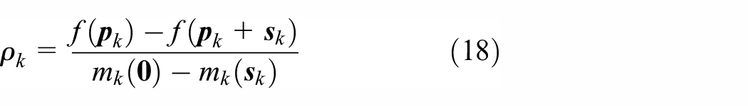
The TRS can be approximately solved by the most efficient dog-leg method ²⁷ to obtain the trial step $s_k$ for the iteration $k$ . Once the trial step $s_k$ is obtained, we need to ensure a good candidate for the next iteration. This is evaluated by the ratio between the actual and predicted reduction of the objective function, that is

$${\rho }_k=\frac{f\left({\mathit{p}}_k\right)-f({\mathit{p}}_k+{\mathit{s}}_k)}{m_k\left(0\right)-m_k\left({\mathit{s}}_k\right)}$$

(18)

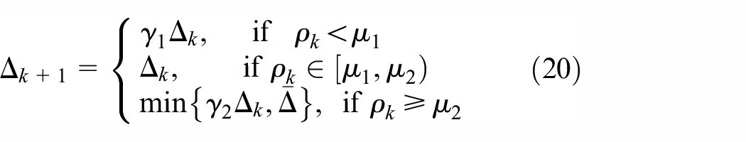
If ${\rho }_k$ is close to 1, the next point ${\mathit{p}}_{k+1}={\mathit{p}}_k+{\mathit{s}}_k$ will be accepted. Otherwise, the trial point will be kept invariant, that is, ${\mathit{p}}_{k+1}={\mathit{p}}_k$ , and the TR will be contracted to derive a more appropriate subproblem for the next iteration. Based on the value of ${\rho }_k$ , the trial point and the TR radius are, respectively, updated by

$${\mathit{p}}_{k+1}=\{\begin{array}{c}{\mathit{p}}_k+{\mathit{s}}_k,\mathrm{if}{\rho }_k\ge {\mu }_1\hfill \\ \multicolumn{1}{c}{{\mathit{p}}_k,\mathrm{otherwise}}\end{array}$$

(19)

$${\mathrm{\Delta }}_{k+1}=\{\begin{array}{c}{\gamma }_1{\mathrm{\Delta }}_k,\mathrm{if}{\rho }_k<{\mu }_1\hfill \\ \multicolumn{1}{c}{{\mathrm{\Delta }}_k,\mathrm{if}{\rho }_k\in [{\mu }_1,{\mu }_2)}\\ \multicolumn{1}{c}{min\{{\gamma }_2{\mathrm{\Delta }}_k,\overline{\mathrm{\Delta }}\},\mathrm{if}{\rho }_k\ge {\mu }_2}\end{array}$$

(20)

where ${\mu }_1$ , ${\mu }_2$ , ${\gamma }_1$ and ${\gamma }_2$ are some empirical constants that satisfy $0<{\mu }_1<{\mu }_2<1$ and $0<{\gamma }_1<1<{\gamma }_2$ . In this article, these constants are set as ${\mu }_1=0.15$ , ${\mu }_2=0.75$ , ${\gamma }_1=0.5$ and ${\gamma }_2=4$ . ²⁷ $\overline{\mathrm{\Delta }}$ is the upper bound of the TR radius.

Before leaving this section, it is desirable to point out that the TR is guaranteed to converge in Yuan, ²⁷ and the proposed method will converge accordingly.

Numerical simulations

In this section, two groups of numerical simulations are conducted to demonstrate the performance superiority of the proposed method. To start, in the first group of numerical simulation, we compare the 2LS and MMA methods in Xu et al., ¹⁵ SDP 2013 in Vaghefi and Buehrer, ¹⁹ SDP 2016 in Zou and Wan, ¹⁴ Classic TDOA in Sayed et al. ² and PAMP in Chen et al., ²⁰ each with the proposed MC-TR method under three typical scenarios. Next, for the second group of numerical simulation, we compare the proposed MC-TR method with the PAMP method to observe their performance as the source node gradually moves away from the convex hull formed by the anchor nodes. Serving as a benchmark when evaluating the performance of various methods, Cramér–Rao Lower Bound (CRLB) derived in Xu et al.^15,28 are also compared.

In order to facilitate peer research and reproduction, the source code used in this work can be found in the Github. ²⁹

The first group numerical simulation

Simulation setup

In this group of numerical simulation, we consider the same source–anchor node arrangement as in Xu et al., ¹⁵ where there are eight anchor nodes and their positions are ${\mathit{a}}_1=[400,400{]}^T,{\mathit{a}}_2=[400,-400{]}^T,{\mathit{a}}_3=[-400,400{]}^T$ , ${\mathit{a}}_4=[-400,-400{]}^T,{\mathit{a}}_5=[800,800{]}^T$ , ${\mathit{a}}_6=[800,-800{]}^T$ , ${\mathit{a}}_7=[-800,800{]}^T$ and ${\mathit{a}}_8=[-800,-800{]}^T$ . Like in Xu et al., ¹⁵ we also put three scenarios into consideration. At the first scenario, we have a monitoring range of $[-800,800]\times [-800,800]$ , and the source node is at $\mathit{p}=[30,10{]}^T$ . At the second scenario, we have a monitoring range of $[-1200,1200]\times [-1200,1200]$ , and the source node is generated randomly within it. At the third scenario, we have a monitoring range of $[1200,3200]\times [-800,800]$ , and the source node is at $\mathit{p}=[3000,10{]}^T$ . In each scenario, ‘small $t_0$ ’ and ‘arbitrary $t_0$ ’ are both considered, as mentioned in section ‘Introduction’.

We set the $K_1$ of the three scenarios as the result of $3.98\times {10}^{-4}$ , $3.98\times {10}^{-4}$ and $5.20\times {10}^{-4}$ multiplied by the area of the scenario, respectively (e.g. the area of the first scenario is $[800-(-800)]\times [800-(-800)]=2,560,000({\mathrm{m}}^2)$ , so the corresponding $K_1=3.98\times {10}^{-4}\times 2,560,000=1019$ , i.e. we first generate 1019 random MC points in scenario 1.) and set $K_2$ as the result of 0.0249, 0.0159 and 0.1656 multiplied by the area of convex hull (rectangle), respectively, which adheres to equation (11). Set $\mathrm{Slt}\_\mathrm{num}\_1=8$ , $\mathrm{Slt}\_\mathrm{num}\_2=5$ and $\eta =0.{001}^2$ in equation (5). The TR method in Yao et al. ²⁴ and Yuan ²⁷ is used to solve equation (5). Then, set the termination condition as $\Vert {\mathit{g}}_k{\Vert }_2<{10}^{-3}$ , where ${\mathit{g}}_k$ is the gradient of $f(\mathit{p})$ at the kth iteration point. For the sake of simplicity, we convert the noise in time domain into distance domain, that is, ${\sigma }_d=c{\sigma }_t$ , and express it in logarithm, that is, $1/{\sigma }^2(\mathrm{dB})=10\log 1/{\sigma }_d^2$ . The SDP-based methods in comparison are implemented by the CVX toolbox ³⁰ using SeDuMi ³¹ as a solver. Six hundred simulation experiments were performed using a personal computer with Intel(R) Core(TM) I5-4590 CPU 3.30 GHz and memory capacity of 8 GB. Root-mean-square error (RMSE) is used to evaluate positioning accuracy.

Simulation results

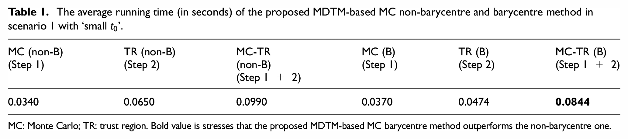
Figure 6 and Table 1 show the performance and complexity of the proposed MDTM-based MC non-barycentre and barycentre method in scenario 1 with ‘small $t_0$ ’. Here, Monte Carlo is abbreviated as ‘MC’, barycentre as ‘B’ and trust region as ‘TR’. The average running time of the compared algorithm corresponding to Figure 6 is listed in Table 1, where ‘MC (non-B)’ denotes the time consumption of MDTM-based MC non-barycentre method (Step 1), ‘TR (non-B)’ denotes the time consumption of the TR method to refine the rough initial position value attained by MDTM-based MC non-barycentre method (Step 2) and ‘MC-TR (non-B)’ denotes the time consumption sum of MDTM-based MC non-barycentre method and TR method (Step 1 + 2). These notations are also applied in barycentre method. It can be seen that both the positioning performance of MC TR (non-B) and MC TR (B) that we proposed can reach CRLB. The final positioning performance of MC-TR (non-B) and MC-TR (B) is the same, but the computational complexity of the later is lower. As can be seen from Figure 6, this is because the initial positioning accuracy of MC (B) is higher than that of MC (non-B), which leads to a reduced time consumption in the subsequent TR search. Note that in subsequent simulations, we will not compare the performance of non-barycentre method.

Figure 6.

Comparison of the positioning accuracy of the proposed MDTM-based MC non-barycentre and barycentre method in scenario 1 with ‘small $t_0$ ’.

Table 1.

The average running time (in seconds) of the proposed MDTM-based MC non-barycentre and barycentre method in scenario 1 with ‘small $t_0$ ’.

MC (non-B) (Step 1)	TR (non-B) (Step 2)	MC-TR (non-B) (Step 1 + 2)	MC (B) (Step 1)	TR (B) (Step 2)	MC-TR (B) (Step 1 + 2)
0.0340	0.0650	0.0990	0.0370	0.0474	0.0844

MC: Monte Carlo; TR: trust region. Bold value is stresses that the proposed MDTM-based MC barycentre method outperforms the non-barycentre one.

Figures 7 and 8 show the positioning accuracy performance of all compared algorithm under all three scenarios and two cases with regard to $t_0$ , respectively. As can be seen from Figures 7 and 8, the proposed MC-TR method outperforms other compared method in terms of positioning accuracy. It is worth noting that SDP 2016 cannot handle circumstances where the source node is located at positions outside the convex hull of the anchor nodes; therefore, its implementation in the second and third scenarios was not shown. However, MMA and SDP 2013 can only handle cases with ‘small $t_0$ ’; therefore, cases with ‘arbitrary $t_0$ ’ are not shown. Due to the randomness of the source node in scenario 2 (including both ‘small $t_0$ ’ and ‘arbitrary $t_0$ ’ cases), we compute the average CRLB in Figures 7(b) and 8(b). Table 2 illustrates the advantages of the proposed method in terms of computational complexity. Although PAMP method has slightly lower computational complexity in scenarios 1 and 2, there are obvious reductions in positioning accuracy performance in scenarios 2 and 3. This is because the Lyapunov stationary point obtained by PAMP method in scenario 2 is sometimes the local minimum or saddle point, rather than the true global minimum point. On the contrary, in scenario 3, the obtained Lyapunov stationary point is always the local minimum or saddle point. More importantly, although the localisation results of other methods can also be refined to achieve CRLB using the TR method, the total computation complexity will increase simultaneously to a lager value.

Figure 7.

Comparison of the positioning accuracy of the proposed MDTM-based MC-TR method with other compared algorithm with ‘small $t_0$ ’ in (a) scenario 1, (b) scenario 2 and (c) scenario 3.

Figure 8.

Comparison of the positioning accuracy of the proposed MDTM-based MC-TR method with other compared algorithm with ‘arbitrary $t_0$ ’ in (a) scenario 1, (b) scenario 2 and (c) scenario 3.

Table 2.

The average running time (in seconds) of the proposed MDTM-based MC-TR method and other compared algorithms in all three scenarios and two cases with regard to $t_0$ .

Comparison conditions	Scenario 1 (small $t_0$ )	Scenario 2 (small $t_0$ )	Scenario 3 (small $t_0$ )	Scenario 1 (arbitrary $t_0$ )	Scenario 2 (arbitrary $t_0$ )	Scenario 3 (arbitrary $t_0$ )
MC (Step 1)	0.0378	0.0667	0.0925	0.0369	0.0691	0.1038
TR (Step 2)	0.0542	0.0937	0.1306	0.0592	0.0954	0.1114
MC-TR (Step 1 + 2)	0.0920	0.1604	0.2231	0.0961	0.1645	0.2153
2LS in Xu et al. 15	0.5467	0.5507	0.5979	0.5493	0.5485	0.5725
MMA in Xu et al. 15	0.2973	0.3156	0.3275	Null	Null	Null
SDP 2016 in Zou and Wan 14	0.9500	Null	Null	0.9557	Null	Null
SDP 2013 in Vaghefi and Buehrer 19	0.3094	0.3259	Null	Null	Null	Null
Classic TDOA in Sayed et al. 2	0.4122	0.2172	0.2247	0.4164	0.2154	0.2164
PAMP in Chen et al. 20	0.0016	0.0565	0.2259	0.0016	0.0535	0.2235

MC: Monte Carlo; TR: trust region; SDP: semidefinite programming; TDOA: time-difference of arrival; PAMP: proximal alternating minimisation positioning.

‘Null’ denotes that the method cannot deal with the corresponding situation. Bold values are highlight the proposed MC-TR method’s average running time.

The second group numerical simulation

Simulation setup

Considering that in the scenario 3 of the first group of numerical simulation, the PAMP method performance drops sharply at the test position $[3000,10{]}^T$ , we added a comparison between the two methods at test positions $[1350,10{]}^T$ , $[1850,10{]}^T$ and $[2350,10{]}^T$ in this group of numerical simulation. The position arrangement of anchor nodes is the same as that of the first group of numerical simulation. Figure 9 shows the arrangement of eight anchor nodes and four source nodes test positions. $K_1$ and $K_2$ are of the same in value as in the first group of numerical simulation in scenario 3. Note that the proposed MC-TR and PAMP methods are insensitive to the value of $t_0$ , and in this group of numerical simulations, we only compare their performance under the ‘small $t_0$ ’ case.

Figure 9.

The arrangement of eight anchor nodes and four source nodes test points used in the second group of numerical simulation.

Simulation results

Figure 10 shows the positioning accuracy performance of the proposed MC-TR and PAMP method in test positions $[1350,10{]}^T$ , $[1850,10{]}^T$ , $[2350,10{]}^T$ and $[3000,10{]}^T$ . As can be seen from Figure 10(a), the proposed MC-TR method has the same positioning accuracy performance as the PAMP method, and they both reach CRLB. However, at test position $[1850,10{]}^T$ from when the signal-to-noise ratio (SNR) is larger than 15 dB, PAMP method has some performance reduction. At test positions $[2350,10{]}^T$ and $[3000,10{]}^T$ , the RMSE of PAMP method is 53.19 and 270.59 m, respectively, while the proposed MC-TR method consistently reach CRLB. This is because the Lyapunov stationary point obtained by PAMP method in the two test positions is local minimums or saddle points, rather than the global minimum point. Table 3 illustrates the advantages of the proposed method in terms of computational complexity in the four test positions.

Figure 10.

Comparison of the positioning accuracy of the proposed MDTM-based MC-TR method with PAMP in the second group of numerical simulation at (a) [1350,10], (b) [1850,10], (c) [2350,10] and (d) [3000,10].

Table 3.

The average running time (in seconds) of the proposed MDTM-based MC-TR and PAMP method in the second group of numerical simulation.

Comparison conditions	Test position 1: [1350,10]	Test position 2: [1850,10]	Test position 3: [2350,10]	Test position 4: [3000,10]
Proposed MC-TR	0.1524	0.1741	0.1954	0.2231
PAMP in Chen et al. 20	0.1543	0.2408	0.2535	0.2259

PAMP: proximal alternating minimisation positioning.

Conclusion

The TOA-based asynchronous source localisation approach in WSNs is examined. Due to the lack of perfect time synchronisation, the unknown parameter $t_0$ makes localisation problems more difficult to solve. We proposed a second-order MC method based on MDTM to obtain a rough initial position result and then refined the obtained result using the TR method. Simulation results show that the proposed method is superior in both positioning accuracy and computational complexity to the state-of-the-art method. However, one theoretical limitation of this work is that algorithm complexity increases slightly as the sensing range increases, although it still works well in a large enough sensing range in practice. In future studies, it is advised to do the further researches on the performance improvements of asynchronous source localisation in non-LOS environments.

The theoretical contribution of our work is that we proposed a new method for asynchronous source localisation based on TOA measurements. The practical contribution of our work is that the proposed method can reach the optimality benchmark of CRLB with low computational complexity.