
Abstract
With the continuous development and cost reduction of positioning and tracking technologies, a large amount of trajectories are being exploited in multiple domains for knowledge extraction. A trajectory is formed by a large number of measurements, where many of them are unnecessary to describe the actual trajectory of the vehicle, or even harmful due to sensor noise. This not only consumes large amounts of memory, but also makes the extracting knowledge process more difficult. Trajectory summarisation techniques can solve this problem, generating a smaller and more manageable representation and even semantic segments. In this comprehensive review, we explain and classify techniques for the summarisation of trajectories according to their search strategy and point evaluation criteria, describing connections with the line simplification problem. We also explain several special concepts in trajectory summarisation problem. Finally, we outline the recent trends and best practices to continue the research in next summarisation algorithms.
Keywords
Introduction
Geolocation is a technique that makes possible to give a position to an object by identifying its geographic position on the Earth at a moment in time. It can be achieved by external sensors that allow tracking (radar, Light Detection and Ranging (LiDAR) and video) or using internal sensors (global navigation satellite system (GNSS)) that achieve their own geolocation.
It is a technique that has existed since the 1950s in the military and space fields. Nowadays, it is accessible to everyone in tiny devices with high precision at low consumption and manufacturing costs. This has progressively made the applications of the technology spread to all sectors: from military tasks such as precisely locating the position of a fighter jet, to transport uses like monitoring cargo shipments or surveillance of endangered animals, and to everyday and everyone functions such as the use of the Global Positioning System (GPS) navigation system in their cars (164 million people in the United States use it in their mobile phones).
This increase in existing information related to geolocation allows it to be exploited using data analysis approaches, like machine learning and big data, making it possible to obtain new knowledge. It can be applicable at different levels to improve and refine intelligent systems.
By grouping geolocation measurements of the same object ordered in time, it is possible to generate trajectories that represent the movement of the geolocated object. According to Zheng, 1 there are four types of trajectories depending on the object that perform the trajectory (people, vehicles, animals or natural phenomena).
It is estimated that by 2022 there will be 29 trillion connected devices in the world, with more than 62% of them being related to the Internet of Things (IoT). 2 Among today’s devices, GPS typically has a refresh rate of 10 Hz, which means that trajectories of long duration can become very heavy. In fact, one experiment 3 proved that storing the GPS records of 400 cars monitored throughout the day costs approximately 100 MB per day.
This implies that the available trajectory information is enormous, meaning a time and processing capacity cost that may be too high. In addition, the use of particularly long trajectories can result in failures of the data mining techniques due to the inability to analyse the details of the trajectory. One recommendable approach in data mining of trajectories is the decision into smaller parts (segments) simplifying the search for patterns of interest. 1
Hence, it appears the need to summarise trajectories in a way that makes the information stored in the trajectories more processable and useful. This new term introduced in this work covers a whole spectrum of other closely related terms, such as trajectory compression or trajectory segmentation. When summarising trajectories, the simplest approach is data compression, specifically trajectory compression, which seeks to reduce the amount of data stored to obtain a trajectory with less weight when it is processed, stored or sent, reducing costs in each aspect and speeding up any trajectory processing algorithm.
Trajectory compression algorithms stem from line simplification algorithms. With the ‘birth’ of computing, there were many uses of vectorial figures: representation of maps, drawings for printing and so on. The computational constraints were much greater than they are today. As a result, the various tasks could not deal with high-resolution data, making it necessary to simplify the lines and polygons used. Researchers as Bellman, Douglas–Peucker, Jenks, McMaster, and many others addressed that problem.
Today, such computational limitations are not that relevant, and the problem has changed by having an additional dimension with the timestamp of the trajectory. Therefore, the current trend in the literature is no longer to summarise trajectories to reduce the storage resources. The objective is to discover new knowledge from this summary moving from these compression techniques towards trajectory segmentation techniques that summarise them using segments that are representative of the different parts of the trajectories and provide a semantic description. This trend does not negate older techniques that only sought to compress as there are many approaches that use compression techniques to obtain representative segments.
Advancing from the more simplistic approach of the line simplification problem there is the inclusion of time within the data, which allow the work in time series and trajectory information. In the 2000s, this transition started with Keogh et al. 4 segmenting time series, Meratnia and De By 5 introducing the time dimension in the compression process, and Anagnostopoulos et al. 6 starting the trajectories segmentation.
There are reviews and surveys that cover this problem of summarisation in the literature,7–14 although most reviews address this problem in a tangential way as they focus on more generic problems. The ones that explore this problem are brief and leave aside the compression or segmentation branches. Moreover, they explain the problem from the time series or trajectories point of view exclusively, without addressing the connection and distinction between the two approaches.
Since there are so many different approaches to the trajectory summarisation problem and the absence of a review that covers them all from a point of view that summarises the whole spectrum, in this article a review and classification of the literature is attempted. This article considers the whole spectrum of trajectory summarisation, focusing on compression and segmentation techniques.
This study of the literature has collected 162 summarisation algorithms. All of them have been analysed and classified within parameters extracted after the analysis of each paper and algorithm design that cover both segmentation and compression algorithms. In addition to algorithms classification, the tests proposed for each algorithm are studied to check whether their performances have been proven to be predominant in the literature. This complete study of each algorithm can be found and download at the website: 15 https://danielamigo.github.io/trajectorySummarisationReview/. It allows to compare these algorithms through the parameters, thus better understanding their similarities and differences.
It has been observed that, although these two approaches to the problem of summarising trajectories exist (compression and segmentation), the algorithms used for both approaches are similar and have many characteristics in common, being two of the most important characteristics:
The search strategy consists of the methodology used to study the whole set of all raw trajectory points. Depending on the strategy, a higher or lower quality representation can be obtained, but it will affect the computation time needed to obtain the summarisation.
The evaluation criteria which are the method used to evaluate whether each subset of the points studied by the strategy should belong to the raw trajectory. This preservation criterion gives priority to one type of result in terms of the summarisation to be obtained, so it is important to choose it according to the problem to be solved.
During the literature study, certain special algorithms were found that approximate the problem with unique characteristics. For example, there are lossless compression algorithms that are focused on not losing information when summarising the trajectory, or algorithms to summarise trajectories considering the road networks on which they move. We also find summarisation algorithms aiming to generate knowledge directly. Known as semantic summarisation, they generate segments with a specific behaviour. This behaviour can be related to the movement dynamics, for example, high-, or low-speed segmentation, or related to the context, for example, stopping near a specific location.
In addition, our literature review pointed out other common characteristics, showing a trend change over the years in the algorithms, which should prevail in future works. For instance, the shift from the data used for the summarisation, adding other dimensions like the temporal data, the need to obtain the summarisation quickly or even in real time, or the search of the best parameters of the algorithms to obtain good results.
This work does not intend to conclude which algorithm is the best for each use, as it is an impossible task. It is necessary a specific analysis depending on the intended use and data characteristics to decide the best one according to the needs of each problem: online or batch compression, limited computational power, mobility constraints such as roads, prioritisation of other variables such as orientation or semantic content and so on. Still, one way to identify how good is a particular algorithm is to check its paper’s comparisons with other algorithms (column ‘Comparison to other algorithms’ on the website 15 ). In order to facilitate the navigation through the many algorithms, a brief and general summary of the overall findings of this work is provided as follows:
Overall, this study concludes that the traditional line simplification algorithms, such as thewell-known Douglas–Peucker algorithm, are outdated for trajectory summarisation, as there are plenty alternatives that provide improved results across all metrics.
Algorithms with probabilistic models of the trajectory movement are promising solutions. For example, self-adaptive online trajectory sampling (SAOTS) or interacting multiple model (IMM) provide good results. Note also that they are capable of producing semantic content. Alternatively, without modelling their dynamics, window strategy–based algorithms such as SQUISH-E or opening window-time ratio (OPW-TR) perform well, achieving a good balance of computational cost with easy tuning parameters.
If it is not required a real-time operation, batch solutions are preferable to online solutions. Among this type, the ones that perform a graph-based strategy stand out. Algorithms such as directed acyclic graph based online trajectory simplification (DOTS) or multiresolution polygonal approximation (MRPA) obtain suboptimal solutions with reasonable computation times.
The main contributions of this review can be summarised by the following aspects:
An introduction and motivation of the trajectory summarisation problem and its links with trajectory segmentation and compression techniques.
An accessible global classification of all types of trajectory summarisation, focusing in two aspects: the search strategy and the evaluation method for selection of key points.
A compilation of notable approaches found in the literature for specific sets of algorithms.
A compilation of common features to all algorithms found in the literature, introducing important trends to preserve in future works.
The remainder of this article continues as follows. Section ‘Basic concepts’ introduces some basic concepts of trajectory summarisation to fully grasp the rest of the work. Section ‘Trajectory summarisation algorithms’ provides the two main categories proposed to classify all the algorithms reviewed. Section ‘Special approaches’ describes several special approaches for trajectory summarisation, while section ‘Other characteristics’ discusses other secondary classifications to highlight trends to be followed in future works. Finally, section ‘Conclusion’ concludes the work.
Basic concepts
In this section, some preliminary concepts are introduced and formally defined to understand the following sections of this article. Table 1 summarises all the notations presented in the section. The concepts are explained supported by the illustration of Figure 1.
Notation summary.


Trajectory example.
Definition 1 (time series)
A list of ordered tuples, being one part of the tuple, the time reference corresponding to the measure magnitude. The other part of the tuple is the measurement itself, which varies according to the problem.
Definition 2 (trajectory)
Time series that stores target localisation data over time. The second part of the tuple is the measurement of the target position at each time instant.
Definition 3 (trajectory point)
A trajectory point is a tuple that stores the measurement of the target at a certain time. Therefore, a trajectory point is formed by two components: the timestamp when the measurement was taken and the spatial location of the target in that time. The spatial information can be represented in local
Definition 4 (raw trajectory)
Original trajectory before any processing is represented as
Definition 5 (summarised trajectory)
A summarised trajectory is a trajectory formed by a subsequence of the trajectory points (selected trajectory points in Figure 1) of a raw trajectory. It is represented as
Definition 6 (segment)
A segment is a subtrajectory formed by two consecutive points of a summarised trajectory. For example, in Figure 1 trajectory,
Definition 7 (trajectory point projection in segment)
Represented as
Definition 8 (compression ratio)
A ratio that measures how much a summarised trajectory is reduced with respect to the raw trajectory. It is measured by dividing the number of removed points of the raw trajectory to form the summarised trajectory with respect to the total points of the raw trajectory. In Figure 1 trajectory, it is
Definition 9 (semantic trajectory)
Summarised trajectory in which each of the segments has a semantic meaning specific to the problem, for instance, uniform, turn, stop and so on.
Definition 10 (summarisation algorithm)
Algorithm used to obtain a summarised trajectory by the processing of a raw trajectory. It needs a search strategy to process the trajectory points sequence and an evaluation criterion that decides if each point should be in the summarised trajectory subsequence.
Definition 11 (evaluation criteria)
The criteria that any summarisation algorithm has. Is used to decide if a trajectory point should be included in the summarised trajectory subsequence or not.
Definition 12 (search strategy)
Methodology that differs between the different algorithms and is used to pass over all the raw trajectory points making the process of the entire sequence.
Trajectory summarisation algorithms
As already indicated, the algorithms that summarise trajectories have the objective of calculating the most relevant points of a raw trajectory to obtain a summarised trajectory. In the whole set of algorithms, two key elements have been found by means of which it is possible to classify the different algorithms, the search strategy and the evaluation criteria to select the key points.
Therefore, to summarise the different algorithms analysed, this section is broken down into two sections:
The first one focuses on the relevant point selection criteria, which summarises the different approaches found when deciding whether to keep or not to keep each point in a subsequence of the raw trajectory within the summarised trajectory.
The second one consists of the processing strategy, and summarises the different approaches found when processing the set of points of the trajectory to evaluate the subsequence to be simplified based on the selection criteria.
Note that these two concepts are not separated but act in tandem to form the algorithm that finds the summarised trajectory.
Figure 2 resumes the different possible classifications that have been found within these two main categories, a trajectory summarisation algorithm may work by combining a strategy with a point selection criterion.

Summarisation algorithms classification.
In each of the following sections, only the most relevant algorithms will be mentioned. At the end of the section, Table 2 indicates where in these categories each of the algorithms studied belongs.
Trajectory summarisation table.

Trajectory point evaluation criteria
As mentioned previously, all trajectory summarisation algorithms need a method to decide whether a point in the raw trajectory should belong to the summarised trajectory. This process is commonly referred to as heuristics. On the simplest criteria it might seem appropriate, although it is not for more complex approaches that are being developed.
This selection of points is usually done by giving a specific score to each trajectory point. This score is based on a specific methodology to quantify by means of a concrete analysis how good a point is compared to another. The strategy will use this score to decide at each moment which point should be included in the summarised trajectory and which point should be discarded.
Throughout the literature review, it has been observed that this category groups the algorithms into the following subcategories according to the methodology used for the selection of these representative points:
Trivial: the most basic algorithm approaches. They do not use any score, only rely on a very basic rule to make the inclusion decision.
Distance: these algorithms use the distance between relevant points in the summarisation process or the trajectory to make the preserve decision.
Velocity: these algorithms use the velocity in points to make the decision.
Angle: these algorithms use the angle difference between several trajectory points to make the decision.
Area: these algorithms calculate areas by merging several points in the summarisation process to make the decision.
Transform: these algorithms are based on the definition of a series of points that mathematically generate a function that approximates the trajectory.
Probability: these algorithms use probabilities calculated by the algorithm itself to make the decision.
Based on multiple criteria: these algorithms combine several of the above criteria to make the decision.
Trivial
Of all the ways of point selection, this is the simplest possible. Unlike the other methods, this method does not perform any analysis of the trajectory characteristics to select the trajectory point to preserve. Instead, it is based solely on a simple selection criterion applied to a list of points.
The first solution in this classification is known as the nth point routine or uniform sampling. Much of the literature gives this application to the work of Tobler.130,131 In this, points are selected with a constant sampling of N measurements, discarding for summarisation the N − 1 measurements in between two selected measurements. In this way, a specific compression ratio is ensured, and segments of a fixed size are obtained.
The other solution found in the literature, instead of relying on a uniform criterion, evaluates each point randomly. On each trajectory point, it applies a random function to decide whether to keep that trajectory point or not. Vitter 132 is the reference that encompasses these approaches. He made a proposal and comparison of line compression using reservoir sampling.
This type of algorithm has the advantage of having a very low execution cost, making it a very simple and fast way to generate a series of segments. Conversely, if these segments have a high level of compression, they will lose the most complex and sharp parts of the trajectory, which is a big drawback for future analyses.
Distance
As mentioned previously, trajectory compression algorithms naturally emerge from the polygonal approximation and line simplification algorithms. The data used by these algorithms consisted only of ordered geometric points which, connected by lines, form figures or polygons.
This approach is therefore the most common throughout the literature, because of the clear importance of a trajectory shape over the plane. The distance is used to compare two points with each other in the same coordinate system. In this problem, distance can be applied to different relevant points, each one being a different approximation.
Trajectory point and segment distance
The most common use of distance is the comparison between the raw trajectory and the summarised one. For each point on the raw trajectory, the distance to the summarising segment can be measured. This distance can be used to detect if the summarised segment after removing some points is not as similar to the raw trajectory as desired. Also, it can be used to choose which point in the trajectory should be preserved. By carrying out this process through all the trajectory points, the strategy will find the summarised trajectory.
The first and logical version of this distance uses the shortest path from the trajectory point to the segment. This distance is the Euclidean distance, known in the literature as Perpendicular Euclidean Distance (PED). It was first introduced with the best-known algorithm in the summarisation literature, Ramer–Douglas–Peucker (DP). Initially proposed by Ramer 133 in 1972 and refined by DP, 114 the DP algorithm makes splits in the trajectory by the trajectory point with the highest PED.
As this metric is measured at trajectory point level, it can be used in multiple ways. DP uses the maximum, but other researchers use it in a grouped form over time, with the metrics Integral Square Error (ISE) 134 and Local Integral Square Error (LISE). 135 ISE quadratically groups all the PED distances of the trajectory. It has a high computational cost but ensures an optimal solution. However, LISE only accumulates the errors of the current segment, ignoring the rest of the segments. Therefore, its solution will be suboptimal, 136 although it has a better computational cost.
This whole process was designed for line simplification solutions. From the 2000s onwards, when trajectories became popular, researchers realised that current algorithms, designed for geometric shapes, were not valid for trajectories. 3 Trajectories are not merely a spatial shape but had an extra dimension with the time at which each trajectory point is measured.
Meratnia and De By 3 introduced a way of introducing the time dimension into the preserve criterion, using its Time Ratio (TR) metric. Instead of calculating the distance of the raw point perpendicular to the segment, it performs a projection of the actual point onto the segment. This projection is calculated by adjusting the time travelled on the raw trajectory and the distance, compared to the distance of the summarised segment. This makes the projected trajectory point maintain the time proportions even on the segment. Later, Potamias et al. 75 made a metric with the same objective but more efficient, called Synchronous Euclidean Distance (SED). The latter is widely accepted by many researchers. The difference between PED and SED distance can be seen in Figure 3.

Trajectory example with PED, SED and consecutive distance.
As with PED, there are the cumulative metrics ISE and LISE, algorithms such as MRPA 44 and DOTS 41 adapt them to SED with integral square synchronous euclidean distance (ISSD) and Local Integral Square Synchronized Euclidean Distance (LISSED), respectively.
Consecutive trajectory points distance
Another way to use distance is to measure the separation between consecutive trajectory points, as it is represented in grey in Figure 3. This value is used by several researchers to check whether one measurement and the next one are separated within a suitable range. If not, it will be necessary to create a new segment.
Resheff 76 does a version of maximum distance between segments radially, integrating also the density of nearby points. Sheng et al. 79 make the same type of radial distance in a maritime environment. Opheim102,137 does something similar, but generates a rectangular area with radial corners, in which, if the following points are inside, they will be compressed.
A middle term between the two distance approaches is created by Dead Reckoning, proposed first by Trajcevski et al. 81 Instead of measuring the distance from the trajectory point to the segment, they establish a predictive zone where the next trajectory point should enter, following the trend of the previous ones. Reumann and Witkam 77 had previously defined a similar concept, where two parallel lines delimit the possible position of the next one to maintain the current segment.
Another way to use this distance between consecutive trajectory points is to measure the accumulation between several of them, taking the length of a given trajectory. This value can be used to compare, as Cui et al. 63 or Sheng et al. 79 do with a maximum segment length limit.
Finally, there are several approaches that use the previous distance concepts but measuring other types of points, which are auxiliary to the trajectory or to the summarisation process. They use to be relevant geographical places for the analysis to be carried out, such as road intersections, 25 regions of interest near the trajectory 138 or even other trajectories. 53 With the knowledge of this distance, semantic content can be generated to be exploited in the future.
Angle
The raw geometric representation of trajectory points allows the generation of more types of metrics to be used during the summarisation process. The angle formed by the relevant trajectory points when summarising can be compared with others along the trajectory.
This evaluation method allows to focus the summarisation process on the preservation of the most delicate components of a trajectory, such as the sharpest angles. There are approaches, commonly called the Direction Preserve Trajectory Simplification (DPTS), first introduced by Long et al., 60 which aim to provide the best heuristics to store this useful information about the vehicle dynamics. As happens in the distance-based metrics, this metric is also applicable to line simplification problems, due to the lack of a time component.
Due to low precision of trajectory data, noise can generate angles that are sharper than they really are. This noise is minimised using the already seen distance metrics but can affect this direction preserving algorithms, preserving such noisy measurements, and discarding the real motion ones. Some specific direction preservation techniques that take this noise into account when dealing with the angles.
Long et al.60,87 proposed several optimal and suboptimal simplification algorithms. Latecki and Lakämper 51 calculate the difference of angles between the previous and the current direction vector. In this case the data are points of a line simplification, to preserve the shape and not to blur the edges.
Wang et al. 139 use the angle formed by three consecutive trajectory points. The angle of the intermediate position with respect to the other two, called by them open angle, when it is an angle far from 180 degrees, represents a sharp turn that must be stored in the summarisation, and calculates the difference of angles between the previous and the current direction vector. In this case the data are points of a line simplification, to preserve the shape and not to blur the edges.
Ke et al. 85 propose a grouping of the difference of the angular values of the vectors, so a change of segment is applied if several trajectory points show a course change by the comparison with a threshold. An example of this algorithm can be seen in Figure 4. Katsikouli et al. 29 perform a different approach, detecting local maximum and minimum angles over time in a way that preserves them.

Example of accumulated angle criterion.
Area
Other method brought directly from line simplification is the calculation of the area (or a volume if has three dimensions) formed by a group of points of the summarisation process.
Visvalingam and Whyatt 111 consider this metric to be more reliable for this type of problem, seeing it as a grouping of distance and angle. Only those that are feasible according to the angle they form (feasible) enter the network. However, it has the disadvantage of being a somewhat more complex and costly calculation to generate.
It should be noted that the distance metrics that calculate a region in which the next trajectory point must be located are not area metrics. Those regions are visual representations to observe if the distance is fulfilled or not, while these calculate a volumetric value to compare with a threshold.
In a similar way to the angle differences, Pikaz and Dinstein 109 use three consecutive trajectory points to calculate the area of the triangle formed between them as a decision criterion. The biggest area central point is eliminated until a threshold is reached. This process is illustrated in Figure 5. A similar variant performs Visvalingam and colleagues.111,140 Later, a modification of the Visvalingam–Whyatt algorithm that includes time in the calculation of the area was proposed. 110
Visvalingam–Whyatt area illustration.
Another common area approximation is to perform Minimum Bounding Rectangles (MBR). These are areas formed by rectangles on a plane, without rotation. The goal of these approaches is to encapsulate all trajectory points in the fewest number of MBRs, minimising the total area. Liu et al. 125 apply it to the plane while Anagnostopoulos et al. 6 do it in a volumetric way, introducing time as another dimension.
The MBRs are a simplified form to calculate the area, since only the base and height of the rectangle are needed. Others62,125 have proposed the metric that realises the area between the raw trajectory points and their projection on the segment of the summary trajectory, although this is only used as a criterion for further analysis, not within the summarisation process.
Velocity
Other way of detecting relevant points in trajectories is the velocity. This metric is completely specific to trajectories (as there is no temporality in line simplification). It should not be confused with SED or TR, which are distance metrics, although they are adjusted according to the time of the measurements.
This metric uses velocity to summarise the trajectory, so it is no longer based solely on position in the plane. This metric is more informed about the dynamics and context of the vehicle’s movement, allowing for more complex, even semantic, analyses. For example, unlike distance, it can detect high-speed variability due to acceleration or angular velocity and segment accordingly. In addition, it allows segments to be generated that, for example, exceed the maximum speed of the area where they are moving, generating useful context in other applications.
When Meratnia and De By 3 introduced the distance TR metric, also created the algorithm Opening Window Spatiotemporal. This algorithm, in addition to using TR, checked a maximum speed differential to perform segmenting, since the vehicle when accelerating or decelerating is in another type of motion. Potamias et al. 75 introduced the algorithm thresholds. It makes a prediction of the zone in which the next trajectory point should appear, but specifically takes the speed into account in the calculation of the valid zone. This ensures that in addition to following the same direction, a constant velocity is maintained.
This is also done using the distance, and the trajectory-point velocity can be compared with the equivalent point projected on the summarised trajectory segment. De Vries and Van Someren 126 use this approach to detect movements and stops, making segments to represent this movement.
Another example of the use of speed in summarisation is that proposed by Lin et al. 117 It uses the Gini index on the velocity values to detect the points at which the trajectory splits. The higher the Gini index, the more different the velocity.
Transform
There are other types of techniques that, instead of using the trajectory points purely for segmentation, they calculate N points that allow, using a mathematical transformation, to reconstruct a continuous approximation of the original trajectory. An example of these evaluation criteria is shown in Figure 6.

Transform criteria example.
These techniques are very common when working with one-dimensional (1D) time series. For example, in audio or electrocardiogram data, but not so much in the trajectories field, which have several dimensions.
However, there is research that tries to apply this concept to trajectories. Rana et al.30,31 and Yuan et al. 27 propose to use Compressive Sensing, to obtain the N-values with which to reconstruct the trajectory. This type of approximation is usually accompanied by a trajectory filtering process to smooth the trajectory and eliminate noise, making it more tractable. Yuan et al. 27 use a particle filter, while Li et al. 141 apply a wavelet transform for each dimension of a maritime trajectory. Long et al. 87 also test the wavelet transform for direction preservation. The fast Fourier transform (FTT) can also be used as simplification criteria, as Katsikouli et al. 29 did to compare its solution.
However, other investigations use splines, polynomial lines that approximate the trajectory. These, unlike the previous techniques, are lines that use the N dimensions. Marino and Manic 99 generate a continuous spline that approximates the entire trajectory. Feldman et al. 34 also use splines, but generate several per trajectory, each one representing a segment of the trajectory.
Probabilistic
All the previous techniques develop a specific analysis based on tangible, measurable, quantifiable metrics. In contrast, the techniques of this grouping perform an analysis with a more complex algorithm, the results of which are probabilities.
These approaches mostly seek to classify each trajectory point as a specific type of movement. By grouping in segments according to the type of movement of the vehicle, more specific segments can be obtained for the type of solution desired. Depending on the type of movement, these segments can be further summarised to reduce the amount of trajectory points.
There are multiple approaches to classify the motion of a vehicle. 142 Siddique and Ban32,33 use Hidden Markov Model (HMM) to classify trajectory points according to whether the vehicle is stationary, varying acceleration or at constant speed. While Garcia et al. 35 use an IMM estimation filter to obtain the type of aircraft manoeuvre, being a solution implemented for air traffic control. 36
Zheng and colleagues127,128 make an analysis of the type of movement (vehicle/walking) of a person within the city, segmenting according to it. The analysis is performed with different inference criteria. Feng and Timmermans 143 perform the same type of problem with a Bayesian Network, having also more types of possible movements.
Multi-criteria
Finally, many researchers choose to combine several criteria to make a much more robust system. This is indicative of the fact that most metrics alone are not sufficient to model and detect all needs. In Table 2, those will appear several times.
Researchers perform the joining of criteria in different ways. Some perform criteria cascading. First, they apply a segmentation algorithm, and then, on the segments found, a technique is applied that finds the most representative points of that segment. Others perform all the checks for each criterion simultaneously. Some, such as the TraClus, 66 use a grouped metric evaluates distance and angle. This follows the Minimum Description Length (MDL) principle, treating the problem as a cost minimisation. Several algorithms follow this same principle. Others, such as online data compression algorithm for trajectories (OLDCAT) 26 or the proposals of Patroumpas et al.73,74 perform different decoupled conditions in parallel, by means of a concatenation of comparisons. These techniques perform online compression to simplify the trajectory and obtaining segments with semantic content.
Something similar is done by Siddique and Ban 32 with self-adaptive sampling (SAS) algorithm. It detects the dynamic variations of the vehicle (constant speed, stopped, accelerate and decelerate) with an HMM and use them to segment the trajectory (Vehicle Flow identification). It also uses a support vector machine (SVM) classifier to detect if the car is stationary (so it is not a trajectory, it does not move).
Others combine preserve criteria in several passes and with a combination of conditionals, such as Feng et al. 115 with speed, distance and angle calculated through the SED projection; or Gao and Shi 94 with angle and SED. Sánchez-Heres 78 does something similar to compress the straight lines but keep the turns.
The heuristics proposed above decide which points to select. But, depending on the problem and its characteristics, it may be necessary to slightly modify the operation of the problem to adjust it. Therefore, several of the proposals perform an additional analysis when choosing the trajectory point to preserve. This analysis is reflected in a weight, a numerical value that can benefit or harm the trajectory points, modifying the final decision criteria.
Li et al. 108 to avoid selecting noisy trajectory points which introduces the weight concept to impair noisy trajectory points. While Kulik et al. 129 instead use weights according to the semantic content it wants to preserve in its compression algorithm. Specifically, it favours the preservation of major roads, while simplifying non-major roads more.
Panagiotakis et al. 53 and Pelekis et al. 144 use a voting criterion among several trajectories by distance between them to find the most representative subsegments of the whole set. Resheff 76 does a version of maximum distance between segments radially, integrating also the density of nearby points.
Search strategy to process trajectory points
As already mentioned, all trajectory summarisation algorithms need a strategy to process the raw trajectory points. The strategy greatly influences the computational cost of the algorithm. The more basic ones only need to pass through each point once, while the more advanced ones increase the order of complexity to a large extent. According to the problem, different solutions can be applied. The challenge is to find a trade-off between computational time and quality of the solution.
Throughout the literature, the following subcategories have been found that depend on the strategy used for processing the trajectory points:
Sequential: these algorithms follow the simplest processing strategy, going through the trajectory points in order, analysing one after another.
Window: these algorithms are based on the use of windows that group several trajectory points, making the decision on the set of points. There are two main variants: a Sliding Window which moves along the trajectory, or an Opening Window that gets bigger and bigger by adding new points to the evaluation.
A variant of the latter is the use of estimation, which is slightly different from the previous ones. In this case, the window checks whether a future estimate of the next points falls within the window.
Split: these algorithms are based on a segment division strategy. An initial segment of the raw trajectory is created, and it is checked if any trajectory point of the raw trajectory exceeds a threshold. If so, the segment will be split in two and the process will continue iteratively.
Merge: these algorithms are the opposite of the split-based algorithms. Their objective is to start from a sequence of segments and merge two of them consecutive using a threshold criterion.
Graph: these algorithms are based on the generation of a graph associated with the trajectory in which the nodes represent points of the trajectory and the edges represent the possible segments.
Once the graph is generated, the summarised trajectory is created by finding the best path within the graph.
Strategy combinations: these algorithms combine several of the previous strategies to make a more robust and intelligent approach.
Sequential
Trajectories are like chains, whose behaviour depends on previous measurements. Therefore, they should be measured considering the previous and ideally also the subsequent behaviour.
This category passes through all the trajectory points in the simplest way, only once and in an orderly fashion through each of them. This strategy is used by researchers to analyse step by step whether the trajectory point should be stored or not (decided by the score provided in section ‘Trajectory point evaluation criteria’), without making double passes or comparisons by accessing previous measurements. This criterion allows to obtain the best possible computation time, but the solution will have a reduced quality, since it does not make enough checks as others do.
It should be noted that this procedure is the one followed with the proposals that perform external and probabilistic analysis. It also models solutions composed of many algorithms that need to extract values initially, for which they make a first pass through all the measurements.
Techniques that aim to find segments representing a motion pattern usually employ this approach. This allows the movement along time to be analysed. Siddique and Ban 32 achieve this through probabilistic algorithms, while Wang 26 does it with a multi-variable analysis.
Graph
The sequential solution allows a solution to be found quickly, carrying out an analysis for each trajectory point individually. Even so, such a strategy is not ideal for any problem, as its analysis does not have the capacity to contemplate previous situations that could be positive for the summarisation.
The opposite approach to sequential solutions is the one proposed by graph approaches. A graph models the entire search space, meaning all possible possibilities of the problem, to find its optimal solution. Graph-based strategies achieve an optimal approximation result but at a higher computational cost than others.
In this problem of summarisation of trajectories, a Directed Acyclic Graph (DAG) is used, where there is a predefined direction from the beginning to the end of the trajectory. The nodes of the graph represent each trajectory point, while the vertices represent the summarisation performed between two trajectory points, discarding the intermediate ones (see Figure 7).

Graph strategy example.
Imai and Iri 42 proposed a DAG by measuring all distances between points of a line simplification, finding the optimal solution by minimising the error, but the computational costs are too high for any solution. It was improved according to the type of problem by Chan and Chin, 43 making it feasible for some non-priority problem.
This type of solutions can also be used to find the optimal solution without using distances as a criterion. For example, Long et al. 60 implement a DAG that uses angular deflection to achieve the best possible summarisation given a maximum deflection. Long et al. 60 also propose a solution (SP, also known as DPTS) in which it makes a graph applied to an angle heuristic, so that it finds the optimal solution.
Optimal solutions are desired in any problem, but in few problems can they be computed because of their high running cost. This makes it impossible to use these algorithms in real-time solutions in any case.
Because of this, some researchers sought to find solutions using graphs capable of achieving suboptimal solutions, but whose computation time was considerably less. Kolesnikov and colleagues49,65,145 were the first researcher to introduce the concept of Reduced Search Dynamic Programming (RSDP) on the simplification problem. In the search for a balance between optimal solutions, called Full Search Dynamic Programming (FSDP) with a reduced computation time. These solutions, instead of generating the entire search space, base their operation on the limitation of the search space to be computed from each vertex node.
Initially, Kolesnikov and Fränti 145 perform the process in a decoupled fashion, initially using a DP to have a reference solution, and exploring alternative paths for each node. He then improved his solution by calculating both the reference solution and the alternatives at the same instant. 49 It used accumulated heuristics as the already explained ISE. Since then, several researchers have opted to follow its path applied to trajectories, seeking to find suboptimal or hybrid solutions, but feasible for real-time use.
Chen et al. 44 were one of the first to apply it to trajectories. His MRPA algorithm uses the accumulation of the SED distance metric, ISSED, to find the shortest path. This solution follows the performance of DAGs, but optimises it computationally using only two queues with priority. Likewise, this solution requires the computation of all distances before finding the solution, which still penalises its real-time execution. DOTS, the algorithm of Cao and Li 41 solves this problem, being able to generate the DAG with ISSED in an online and incremental way. Wu et al. 55 also explore real-time graph solutions and compare them.
Another more specific type of solution is proposed by Pulshashi et al., 54 this one is not so much focused on compression, but on generating segments by eliminating atypical trajectory points due to noise. To do this, the DAG it generates introduces, for each trajectory point k new vertices, to the next k nodes. Moreover, with these k additional paths per segment, it can develop the algorithm in real time.
Window
Knowing that optimal algorithms are not a feasible solution for virtually any solution, many researchers opted for other heuristic paths. These seek to find a path by performing without generating a DAG, but by traversing the trajectory in other ways. One of these uses a window that limits the search space to a sequence containing a few trajectory points. This causes the preservation criteria checks to be performed only between such measurements, thus making the checks much fewer.
It should be noted that the sequential concept can be viewed as a window of size 1. This concept of evaluating all consecutive points makes clear a linkage to be able to run the algorithm in near real time, having to store a few measurements to extract results. There are two types of approaches using the window concept to traverse the points.
Sliding window
For a particular trajectory point of the trajectory, N of the neighbours of that point are selected and the calculations are performed with them. The placement of the window with respect to the point can vary according to the algorithm: placing it in an intermediate way and taking points before and after or taking only points on one side.
Once the operation of the window is established, the behaviour of the window depends on the algorithm that implements it. The trivial algorithm of Tobler130,131 can be seen as a window of fixed size. The same is true for the Pulshashi et al. 54 with graphs, which generates k vertices for each point, where k is the size of the window.
Keogh et al. 146 proposed a sliding window implementation for time series. It checked the error in distance of the segment formed by the window, with respect to the intermediate trajectory points. If they exceed a threshold, it splits, otherwise it shifts the whole window, discarding them from the summarised trajectory.
Yan et al. 112 instead use the window to find and classify fragments of the segment according to the type of movement. Thanks to the window you can apply it in real time.
The solution of Muckell et al.,100,101 SQUISH, uses a window of N measurements. On these N measurements, it chooses the worst one and eliminates it, inserting the next one and so on until the trajectory is finished.
Marino and Manic 99 use the Window to quickly calculate the direction correlation of the trajectory points. Finally, Gao and Shi 94 use a window on which you apply several criteria at the same time.
Opening window
Alternatively, the window can be viewed as a point buffer, where as long as a criterion is active, trajectory points continue to be entered. When the criterion is no longer met, the window starts again. Depending on the implementation, either at the last point of the window, which is preserved in the summarisation, or at the last current point of the summarised trajectory.
The first reference found in the literature that applies an opening window is the proposal by Shatkay and Zdonik, 147 applied over time series. Although the main author of this approach is Meratnia and De By, 3 which introduced the name of this concept, opening window. In addition, Meratnia and De By 3 differentiated between two variants, whether to stay with the point that exceeds the window, or the point just before (Normal OPW), where the window has not been exceeded (Before OPW). Another variant to find the specific point is that of Meng et al., 70 which after applying the window with a criterion, uses a cumulative SED distance to find the exact point to store in the summarisation, and continues from there.
Many researchers followed this type of trajectory approaches, for example, Lee et al. 66 and Sheng et al. 79 The segments are then generated with their multi-criteria metrics, until it exceeds a threshold. The same is done by Liu et al. 89 using speed as a criterion.
Direction estimation algorithms are also related to opening windows. The algorithms fix an orientation and all points that fall within this window are not selected for the summarised trajectory. As this enters algorithms such as Reumann and Witkam 77 establishing two infinite parallel lines, Opheim102,137 with a delimited area or even Dead Reckoning 81 and its variants Connection-Preserving Dead Reckoning (CDR),50,148 which also recalculate the intermediate points of the window at each iteration, in case it moves far enough away from the current point vector.
Kolesnikov 65 does something similar, setting an area where the point can be as a prediction, and the following points must be within it. In addition, thanks to the window, it performs the combination of the areas of past points, obtaining a more accurate estimate.
Split
Another strategy to go through all the points quickly is the Split method. This method is based on Dynamic Programming, generating a recursive way of dividing the global problem, and solving it in smaller pieces. Also known as divide and conquer, or top-down, the objective of this strategy is to split the trajectory by the most relevant point according to a criterion. With this process, two subsegments are generated, one from start to the selected point, and the other from this point to the end. These two segments, in turn, apply the same problem again, generating the recursion. In this way, the trajectory is segmented until it reaches a previously established limit. This approach gives fast results, but its way of traversing the trajectory points prevents it from working in real time since it needs to process the whole trajectory.
The most known algorithm of summarisation, Douglas and Peucker 114 (DP), uses this strategy with a PED distance threshold. Thanks to it, multiple researchers have tried to improve it. For example, Hershberger and Snoeyink 116 proposed a variant with the same result but faster, called DP-hull.
The algorithm Scan, Pick and Move (SPM) 120 is a variant similar to DP, but instead of generating two segments on which it is necessary to reapply the algorithm recursively, it keeps fixed the first of the two segments generated, applying recursion only on the second segment. This provides on long trajectories a faster solution, but at the same time the result will be worse and does not guarantee a maximum error.
Like all strategies, the split-based can also implement any type or combination of point preserving criteria. For example, Liu et al. 125 use it to minimise the area of the MBRs that encompass the trajectory points of a trajectory.
Merge
The opposite way to Split can also be applied on trajectory data. Instead of starting from the general problem and going to multiple specific problems and finally joining the solutions, the merge algorithms start from multiple specific problems and arrive at the solution of the general problem. This strategy is also considered as Dynamic Programming, it starts with segments of few trajectory points and the algorithmic process oversees finding which pairs of segments can be joint together in bigger ones.
This process is also known as Bottom-up, or elimination, because, when joining segments together, there is a trajectory point that is discarded. Unlike the Split strategy, this one can be applied in real time with several nuances.
Pikaz and Dinstein 109 performed the first appearance of Bottom-up in this type of problems, applied to polygon approximation. Hunter and McIntosh 149 also applied it in time series. Visvalingam and Whyatt 111 apply this concept also with an area criterion. It starts with trios of trajectory points and eliminates the intermediate point of each trio when it has the least area of the whole trajectory. In this way, the trio that has been eliminated disappears, and the others are modified, using the closest point that has not been eliminated.
In trajectories it is possible to highlight, SQUISH 100 and its improved version SQUISH-E 101 which are two of the recent algorithms with the greatest impact in the literature. Both use a merge strategy, mixed with a sliding window to minimise the SED distance. The algorithm is highly configurable and can be set to minimise the error while maintaining a specific compression ratio, or the opposite, to maximise the compression ratio while keeping the error below a specific value.
Another similar solution with merge strategy and window is the one performed by the algorithm STTrace. 75 It first fills a buffer and then removes the one with the worst SED. Li et al. 108 also execute a merge strategy, eliminating the points with the highest weight, calculated in a multi-criteria way.
Strategy combinations
Finally, as is also the case in trajectory point preserve criterion, strategies can be combined with each other to realise solutions with different objectives. In Table 2, those will also appear several times.
The need for graph algorithms to limit their computation time in order to achieve a suboptimal but fast computational solution was discussed earlier. This effect is repeated in other types of strategies, already more efficient than a hybrid graph, achieving an implementable solution in IoT boards or low-cost beacons. The opposite effect can also be sought, to find a more specific solution with a more refined result.
Some apply the different strategies at the same time, supporting each other. Sliding Window And Bottom-up (SWAB) is one of the oldest combinations found in the literature. Keogh et al. 4 proposed that union between a window and merge strategy, where the sliding window incorporates points until it fills a buffer, and merge empties the buffer, selecting the most relevant points.
Another interesting mix is the one performed by Liu et al., 125 where it starts from segments of fixed size (number of trajectory points that make up a segment). On them, apply Split or Merge according to the size of the segments, until the MBR area is minimised. The already mentioned SQUISH-E 101 and STTrace 75 are also examples of a combination of merge strategy with a window that limits the amount of information to be processed.
Other approaches do decoupled cascading during execution. These detect, for example, when to store a point, so that a later analysis selects which of the points to store. This is the case of Meng et al., 70 who first applies an opening window until an SED distance threshold is exceeded, but once the threshold is triggered, finds the point to be preserved in Split form, with a different metric.
The same happens in the Generic Remote Trajectory Simplication (GRTS) algorithms proposed by Lange et al. 148 It uses the CDR algorithm to detect the moments to send points, using an opening window strategy. Once out of the threshold, apply another, more accurate algorithm to compress the fragment. It can even run high computational time algorithms online, by reducing the number of measurements it must process. GRTSOpt uses an optimal algorithm such as Imai and Iri, 42 whereas GRTSSec uses a heuristic solution OPW-TR. 3
Finally, the algorithms that perform the cascade in a totally decoupled way. They first make a pass with one strategy and with the results, apply another or other strategies with which to achieve summarisation. A typical cascade approach is by first carrying out a sequential run that extracts values from the trajectory, and then, using these, other algorithm is applied to select the measurements.
Hansuddhisuntorn and Horanont 17 use this approach to reduce the number of trajectory points to be introduced into an algorithm, so that it is less computationally expensive. First, it makes a sequential strategy to choose only relevant points in velocity or angle, and those it inserts into the algorithm Top-Down Time Ratio (TD-TR). 3
Lee et al. 150 make two forward passes. First, it does a coarse partitioning of trajectories separately (using TraClus). Then, with the trajectories potentially outliers, it makes another more specific segmentation by pairs of distinct trajectory segments.
Another example of the use of velocity in summarisation is proposed by Lin et al. 117 As is shown in Figure 8, its algorithm uses the Gini index on the velocity values to detect the points at which the trajectory splits. The higher the Gini index, the more different is the velocity. Then, with the velocity values, find the error threshold to use from PED in a DP to compress for subsegment.

ATS117 algorithm illustration. Multi-criteria by cascade.
DOTS-CASCADE 41 applies the DOTS algorithm N times by parallelising the network computations, so that it can run in real time. A similar approach follows Siddique and Ban 32 using first HMM to locate the important points and then SVM for stops. Other algorithms are based on applying several passes (each pass following a procedure different from the rest) on the trajectory points to acquire knowledge that cannot be obtained by means of a single pass.
Within this last category, a common operation can be identified: algorithms that perform passes of the same algorithm in both directions of the trajectory. One pass from the beginning to the end, called forward, and another in the opposite direction, called backward. This type of strategy is common in probability algorithms, but since there are probabilistic criteria for preserving trajectory points, it allows a more detailed analysis of the target’s behaviour. Although the concept comes from there, some researchers use it to refine the segments without techniques that work with probabilities.
Garcia et al. 35 use an estimation filter called IMM, the result of which lets you know what type of motion the target is performing. If set correctly for a particular type of vehicle, this filter can estimate by probability the type of motion the vehicle is making. The forward pass is responsible for detecting the beginnings of a motion segment, while the backward passes detect the ends. Their union allows to generate informed segments categorising straight, turning, stationary and so on movement.
Liu et al. 98 perform a double pass in time series, where the first Feasible Space Window (FSW) finds the segments following a distance criterion and a sliding window strategy. Then, the backward pass, Stepwise FSW, retouches the position of the segments reducing the representation error of the initial segments of the FSW. This approach allows to make a final pass when the trajectory is completed, so that in real time the segments are suboptimal, but when finishing and storing the results, they are improved with the backward segmenting process.
The same objective has Kolesnikov 65 with its Scan-Along Trajectory Approximation (SATA) algorithm, explained above. By accumulating the areas found by means of an opening window, it guarantees a minimum of error. However, this single pass can be improved by performing another pass in the opposite direction, applying the same window now in the other direction.
Tang et al. 80 and Etemad et al. 91 use a double-pass approximation in a different way. For certain trajectory points, it applies the double-pass concept along a sliding window. With this it checks the velocity (Tang) or the direction (Etemad) of several points before and after to improve the detection. Tang later applies an improved DP for segmentation.
Finally, as summary of this section, Table 2 indicates where each of the algorithms studied in the literature are located accordingly to the categories proposed. Notice that some of them combine several criteria to make more robust solutions, and for that reason, they appear in several places in the table.
Special approaches
Within the trajectory summarisation literature reviewed, in addition to all the groupings above, some special approaches to the problem have been found. These still aim at reducing the dimensionality of the trajectory, but they have an additional motivation that makes their implementation peculiar. The most relevant of these are explained as follows:
Multi-Trajectory Compression (MTC): instead of compressing each trajectory individually, they try to take advantage of the knowledge coming from the existence of multiple trajectories in relation to each other.
Lossless compression: these algorithms stand out for generating the summarised trajectory without any loss of information, being possible to recover the raw trajectory from the summarised one.
Road networks constrain: these algorithms stand out for being specially designed to be used in conjunction with context information from the road network from which the information has been taken.
Semantic approach: these algorithms are notable for including and using semantic information, extracted from the applicable problem, when generating the summarised trajectory.
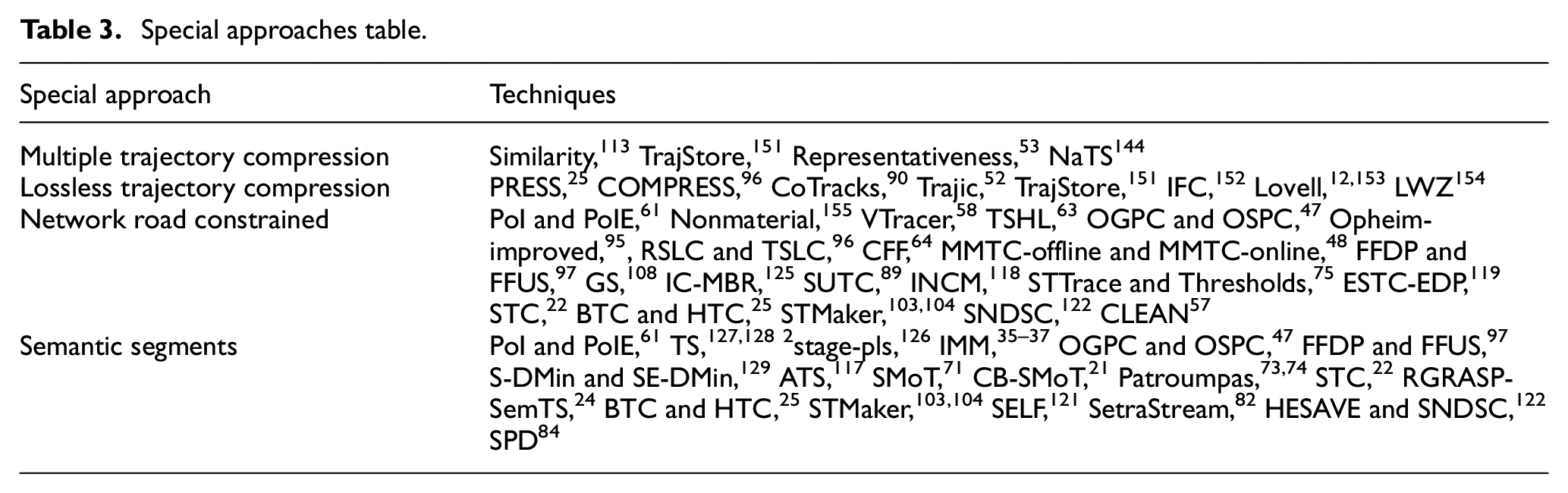
This categorisation is shown in Table 3 and also at website. 15
Special approaches table.
MTC
Trajectories usually have a predetermined destination, and, if such a trajectory takes place with a certain frequency, it usually has the same path that is followed to get from one point to another. These trajectories predominate in urban land navigation, where almost all vehicle movements are on roads or at least dirt roads. In places where movement is not restricted, such as maritime navigation or air traffic, and although less so, a series of prefixed paths are also usually followed on long routes.
There are several approaches that seek to exploit this redundancy of trajectories on the same path to maximise the summarisation and compression of a trajectory. The objective is, instead of compressing each trajectory individually Single trajectory compression (STC), like all previous techniques, to try to exploit the knowledge of existing trajectories with similar shape and dynamics. In doing so, solutions can reduce dimensionality abruptly, going from hundreds of redundant trajectories in shape, to storing only one that represents all of them.
These approaches are usually more related to a complete framework for a posteriori analysis, or clustering techniques, as they require multiple refined trajectories ready to be processed and compared with each other. TrajStore 151 was the first approach to do MTC. It groups virtually identical trajectories by clustering, comparing the trajectories with each other using similarity metrics. When it identifies a cluster, it uses one of the trajectories in the cluster as a representative of that group, saving the storage of the N trajectories.
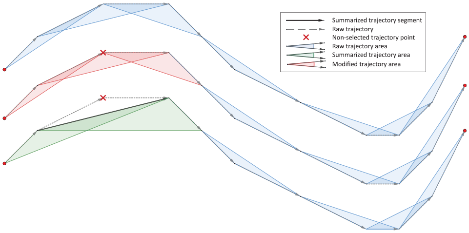
Birnbaum et al.’s 113 technique generates segments for each trajectory using a lossy STC algorithm, and on the other hand tries to represent the trajectory with subsegments of other trajectories already stored. The form that minimises the error will be the one that stores, if the new segments obtained with the compression STC, or it will use the already existing ones in the MTC. It also minimises the replicated information, namely, by storing the start and end time of each segment, since all the intermediate positions can be interpolated from the base segment. In addition, the successive points store only the gaps between measurements and time, not the complete value, to reduce space. This facet is usually related to lossless compression, which is more oriented to databases.
Zheng and colleagues28,156 propose a framework that first eliminates the redundancy of multiple trajectories, keeping only the priority segments, and then compresses each segment separately. To do so, it uses similarity metrics, which compares all trajectory points of both segments with each other.
Likewise, any trajectory subsegment clustering technique, such as TraClus,66,157 could be applied to this criterion. Panagiotakis et al. 53 and Pelekis et al. 144 use a voting criterion among several trajectories by distance between them to find the most representative subsegments of the whole set.
Lossless compression
One of the most common characteristics of summarisation algorithms is the loss of information suffered with the compression of trajectory points. This means that the algorithms manage to generate segments containing new information based on the original measurements, although the generated segments do not represent the original information. This approach is the most common and is called lossy.
However, there is another approach in which the information is compacted without degrading it. This approach, called lossless, makes it possible to preserve the original information while occupying as few bytes as possible. In addition, it must ensure that all the precision of the raw trajectory is recoverable. This type of approach usually gives little importance to the summarisation part and focuses entirely on data reduction, although some techniques do exploit the characteristics of the trajectories.
The simplest example to understand the difference between lossless and lossy compression is to switch to another domain. Images can be lossy compressed into JPEG files, which achieve a very high compression ratio, but generate artefacts in the image that do not exist. However, if compressed in PNG files, lossless compression is achieved in each pixel of the image, although with a lower compression ratio.
Lossless bases its operation on structuring the data in a more efficient way, so that the information is compressed. In addition, it looks for redundant patterns in the information to save space. Transforming the data to such a structure requires extra computation time, and the same for decompressing it again to obtain the original path. These techniques have disadvantages, such as making it difficult to access the trajectories with such intermediate computation, but they have advantages, such as storing the same original trajectory at a lower space cost, useful for long-lived databases.
Lossless compression is a commonly practised term in computing. In fact, the Consultative Committee for Space Data Systems (CCSDS) 158 proposes recommendations and sets the standard for how a lossless compression algorithm should work.
There are two types of lossless algorithms: the generic ones, applicable to any type of computer file with a decent compression ratio. The other approach is to develop a specific solution for the data to compress. Like in the mentioned example with image data, it is possible to develop a specific proposal to deal with trajectory data. Below, solutions in the latter category are presented.
Hatanaka 159 eliminates redundant information, storing only the gaps between measurements, reducing information by up to 80%. Song et al. 25 propose PRESS, a map-matching framework with both trajectory summarisation modes: lossless and lossy. Then, Han et al. 96 proposed COMPRESS that starts from the base proposed by Song and improves it different fields.
TrajStore 151 compresses the trajectory by clustering and saving a representative of each cluster. Later, Trajic 52 claims to have outperform TrajStore approach. Trajic’s paper also develops a different lossy solution, based only on bits encoding.
There are even proposals to combine both forms of compression as Balzano and Del Sorbo 90 does: first a lossy compression is perform. Then, with the selected trajectory points, a lossless compression, so they occupy as little space as possible.
Lovell12,153 has recently made several approaches seeking to exploit kinematic values to perform lossless compression. In addition, the paper provides a clear overview of the lossless trajectory compression status.
Semantic segments
Many approaches in the literature, especially recent ones, aim at generating segments that represent concrete information. These are called semantic knowledge. The trajectories are compiled by GPS sensors, giving a position over time, moving over the Earth. These, in computational form, are tuples of numbers with several decimals, which a human being is not able to understand, at least, without a previous study of the problem.
Therefore, with the aim of making applications for a non-expert public, the transformation of this numerical information into tangible, legible, explainable knowledge is a very well-studied and necessary problem for any application. This knowledge is obtained by means of artificial intelligence techniques, capable of analysing the behaviour of thousands of trajectories and knowing how to differentiate a specific aspect of each one of them.
This review considers the semantic content in trajectories in two ways: first, by generating self-explanatory segments, according to the type of movement the vehicle performs. Or second, by generating additional information related to the geographical context through where the trajectory runs.
OLDCAT, 26 Patroumpas et al.,73,74 Siddique and Ban32,33 or Garcia and colleagues35–37 are authors of approaches that detect the change of trajectory motion type. This implies that they are able to identify the type of motion between two points of change, categorising segments with a particular type of motion.
Previously some algorithms were mentioned aiming to find the start-stops points of the trajectory and compressing with it. These approximations are semantic content. Zheng et al. 84 apply clustering of individual trajectory points to detect stay points. Alvares et al. 71 did something similar, but the detection is done semantically, by placing an area of interest to monitor. When more than one time threshold is found within the area, it is a stop. Between stops, there is movement. It detects interesting trajectory points on ships from the angle of rotation between measurements using clustering. They found this algorithm useful to identify fishing spots.
Tamilmani and Stefanakis 121 use the Semantically Enriched Line simpliFication (SELF) structure to store semantic content, aside from position and time. It specially compresses the semantic content by angle and velocity, allowing it to be interpolated if necessary.
Richter et al. 22 propose a compression in road networks using map-matching, but, unlike the previous ones, it does not store the positions where it is located, but stores the name of the streets it travels, a more understandable way for the human. With this information, it is still possible to decompress and find the real trajectory, together with the time. Su et al.103,104 take it one step further, summarising the trajectory in natural language: its crossing points, average speed in each segment and so on.
Road network constrained compression
There is another type of approximations when the trajectory occurs in a network of roads that limit the trajectory performance. Here the problem of GPS noise is accentuated, appearing noisy trajectory points that go out of the trajectory, being necessary a previous iteration that adjusts these points to the corresponding road. Subsequently, with the points already adjusted to the road, the segmentation/compression algorithms use the context of the road, mainly the intersections, to approximate the trajectory.
Moreover, with the concept of roads, it is not necessary to represent and store the shortest path between two points, but it can be inferred a posteriori if needed, since the possibilities are reduced. This problem could be done with Naïve solutions, combining the two algorithms: Kellaris et al. 48 propose to do compression and then map-matching. Or applying map-matching first, with the points on the road, compress, and then map-matching to the road but taking up less.
Non-material 155 was the first to combine trajectory compression and trajectory map-matching. His solution separates the spatial trajectory, which can be extrapolated from roads, from the temporal component, which belongs to each track. The spatial compression stores the crossing intersections and the temporal gaps between intersection pairs.
Map matched trajectory compression (MMTC) 48 uses subtrajectories through fewer intersections to replace parts of the original trajectory. Some specific evaluation functions are introduced during the compression to guarantee the similarity between the compressed trajectory and the original one. The compressed trajectory consists of fewer intersections; thus, the storage cost is reduced.
Gotsman and Kanza 47 proposed several ways to perform compression in road networks. Using graphs, it finds the shortest path (highest compression), knowing that it can then redo the path (since the path can only pass through the available roads) looking for the shortest path between both compression points. It proposes optimal and even online solutions.
Li et al. 108 work offline, taking into account the confidence in the GPS measurement, so it eliminates outliers. It applies the compressor first and then does map-matching, so it does not link the two phases. Something similar does Cui et al. 63 which first segment with angle and length and then fit the segments to the road.
Liu et al. 89 first do map-matching and then check if the speed is adequate and applies lossless compression. Popa et al. 118 propose another compression method with deterministic error bounds and an error measure for in-network trajectories. It assumes that the noise path has been cleared, and all the points are already on the road.
Other characteristics
As mentioned previously, a literature review with a good number of papers will detect several common characteristics. In this section, they will be introduced and its significance in the most recent studies will be explored. In particular, the following characteristics have been identified:
The ability to segment in real time as soon as the data are available. There are two possibilities, batch mode implies that the complete trajectory data are available after the entire trajectory has been traversed. The online mode means that the data are available in real time, as each measurement is taken, the data are passed to the algorithm for processing.
The type of input data implies the level of trajectory information used. That is, the time component of the trajectory is taken into account, or only the shape of the trajectory.
Finally, due to the flexibility and complexity of these algorithms, it is explored if it is necessary to adjust their parameters accordingly to the problem and the type of trajectories to be summarised.
Like the other classifications, all algorithms are also categorised according to these features. Available at website. 15
Real-time operating
There were two main ways of approaching an algorithm to process data, depending on the availability of the data, it is possible to work in real time as new data appears or offline after all the data have appeared. Working with trajectory data, an offline or batch algorithm, because of its way of processing data, requires all the trajectory points from the beginning of the execution. Having all the information from the beginning allows them to provide potentially optimal solutions to the problem. Meanwhile, a trajectory point buffer can operate in real time, delivering results as more measurements arrive. This needs to provide results in real time means that they cannot claim to find the optimal solution. They must perform a trade-off to obtain a good solution within a computation time that allows processing measurements faster than the time in which new measurements arrive.
Both approaches are useful in a problem as broad as trajectory analysis, which has so many possible uses. For example, in a big data environment, where all the available information from millions of trajectories is available, a batch solution will be preferred, potentially with better results. However, there are use cases where the solution must use an online algorithm. For example, when monitoring a target using a mobile device, it is necessary to process the detections and obtain results in seconds with which to make informed decisions. There is also a middle ground, and it should be considered, when the entire trajectory is available, but the solution has to be delivered with a relatively low delay.
The original line simplification algorithms did not require immediacy in the results to be obtained, as they were static data with hardly any online use cases. In addition, the sensors were less accurate and the amount of information per trajectory was limited. Therefore, most of the algorithms in the literature were batch.
Starting in the 2000s, trajectory summarisation algorithms began to be developed. Initially, they start from line simplification algorithms, but due to the technological advance, other uses have been generated and the literature has covered them. Nowadays, there are many more and more accurate ones. The use cases of these technologies are looking for online solutions that provide segments that represent additional information, beyond the mere compressed line. The accuracy and redundancy in a trajectory are so high that it is not so much necessary to maintain it, and have it taken up less space on the device, as it is to extract useful information for various contexts.
This needs to have solutions as soon as possible has led to a recent trend where researchers try to exploit all the computational characteristics of the devices where they implement their solutions. Currently, processors have multiple cores that allow parallelisation of computation. Others even have dedicated components for high-performance tasks, such as artificial Intelligence (AI)-specific cores or graphics processing unit (GPU) cards with thousands of cores. This parallelisation should be in the design of the online and offline compression algorithms of the future and can accelerate very expensive implementations by many orders of magnitude. Some examples of the parallelisation are the Patroumpas et al.73,74 approaches, graph speed-up by Deng et al., 59 Feldman et al. 34 or Huang et al., 160 or the spin line detection of Feldman et al. 34
Input data
Related to the evolution of the techniques over the years is the evolution of the type of data used by the summarisation algorithms. Most of the techniques initially developed were designed and tested by their authors for two different problems: time series, that is, a variable over time, or line simplification, that is, position only, without time. These were used as the basis for this new branch of research, which relies on the union of position and time.
There is a trend where summarisation algorithms are moving away from using only the trajectory form, making solutions that could also work for line simplification problems, and are incorporating all kinds of additional variables. The first step was to introduce the time component in the calculation to summarise the trajectory, since it is as or more important than the rest of the variables.
The current trend is to try to add another type of semantic knowledge to generate representative segments, both context of the segment with respect to the rest of the trajectory, and of the environment through which it moves, or the difference with respect to other vehicles travelling through the same area.
An important factor for the correct development of trajectory simplification algorithms in the future is that they correctly take time into account. Algorithms that do not consider time and are based solely on shape are outdated for most of the analyses to be performed. They are clearly inferior for any trajectory problem.
Need to adjust parameters
Most of the summarisation algorithms have parameters that can be adjusted to obtain a correct performance. For this, an analysis of the type of trajectories to be simplified, the characteristics of the algorithm and each parameter is necessary before running it.
Most of the works presented above perform the adjustment of parameters by hand by trial and error, making modifications of the parameters until an acceptable solution is found that represents a local optimum. Some examples are Zhao and Shi 161 or Amigo et al. 162 which perform an empirical manual analysis of the threshold fit to find the best segmentation.
However, some algorithms do not perform a manual study but have an automatic and unsupervised adjustment of the parameters. Liu et al. 20 automatically fit it inside a DP, for the maritime context. Something similar can be observed in the study of Zhang et al. 163
Many parameters to make it work properly. Some researchers use multi-objective evolutionary techniques to fit the parameters within their problem.164,165
In Shuang et al.’s 166 solution, an automatic speed threshold is calculated within segments for anomaly detection. While Wei et al.’s 107 solution uses statistical theory is applied to determine thresholds for course variation and speed variation.
Soares et al. 23 use MDL to avoid the use of thresholds. This solution selects N points randomly as representative points, similarly to a clustering approach, and automatically adjusts itself by means of the cost function formulated with MDL.
Summarisation evaluation
Since there are so many algorithms and approaches that summarise trajectories, it important to analyse the performance of each algorithm in the different problems, being capable of comparing them to select the most suitable for each case.
Some of the articles reviewed do not make any evaluation of the performance of the algorithm, especially when summarisation is merely a step towards another end purpose. This practice is undesirable. It is essential to always be informed whether the segments met the qualitative and quantitative needs of the next step in order to guarantee the results will be achieved. This work analyses which metrics they use to evaluate its work, against which algorithms they compare its solution and which type of trajectories data is used as input.
Metrics
For the evaluation, many evaluation metrics have been used in the reviewed literature that check how well a compressed trajectory (or the generated segments) approximates the real trajectory. Those metrics can be divided into the following categories:
Summarisation meta-information: metrics that compare the raw and summarised trajectories regardless of the trajectory factor. Metrics such as compression ratio or bytes reduction are metrics in this category.
Algorithm computational complexity: these metrics seek to measure the computational efficiency of each algorithm, by checking the execution time or memory consumption.
Error metrics: metrics that calculate an error residual between the actual trajectory and the summarised trajectory. The most common way is to adopt the trajectory point preserve criterion used alongside a statistic values (average, maximum, etc.).
Similarity metrics: using specific metrics that compare two trajectories (or segments) to see how different they are. Some works use this metrics comparing the real trajectory and the summarised one.
Comparison to other algorithms
This article also explores how works benchmark their results against others in the literature. This is the only way to demonstrate if an algorithm performs well or not for a specific problem (the problem described on each paper).
Most papers do not compare themselves against other algorithms in the literature, showing only the results they achieve. This lack of knowledge of the existing literature on the problem means that many researchers consider its approach innovative when it is possible that previous work did it earlier. Moreover, it is possible that another algorithm in the literature can perform better for the same problem. Column ‘Comparison to other algorithms’ on the website 15 shows the comparison provided in the paper that introduces each algorithm.
This review provides an initial overview of multiple existing approaches in different categories, facilitating the decision of with which algorithms a future work should be compared. Also, a set of highlighted algorithms is also provided in the introduction according to the type of solution desired.
Data sets used
A proper evaluation of a summarisation algorithm requires that others can evaluate their algorithms on the same set of trajectories and benchmark it against them.
Throughout the literature, there is a clear predominance of trajectories in cities. This is logical, as this is the domain where the majority of travel occurs for humans. This also leads to the existence of many specific algorithms for such trajectories. Some algorithms use real experiments with their own data, but several public data sets stand out in the literature.
GeoLife 167 is a data set that is developed in a city, with trajectories categorised according to the motion method: vehicles, bicycles or people walking. Data sets of taxis or trucks moving through a city are also common. Data sets of taxis 28 or trucks 62 moving through road networks are also common.
Other researchers use ship data. AIS technology is a simple approach to data set generation, as it is an open standard by which ships are required to communicate their position. There are multiple data sets that collect information from AIS detections in specific areas. 168 These data also incorporate contextual information such as ship type or destination, allowing for easy post-summarisation analysis.126,169 There are other types of trajectories that are less used but noteworthy. Among them, there are some hurricanes data sets, 91 with a more limited amount of information, but with very different behaviours from the rest of the trajectories. Finally, the trajectories of tracking animals: such as deers 60 or bats. 68
Conclusion
In this article, an overall review of trajectory summarisation algorithms was provided, merging both compression and segmentation concepts in a same perspective. This type of approach has not been explored in any of the existing surveys available in the literature.
The concept of summarisation and its application in different use cases has been introduced. These have two main motivations: the need to shrink or simplify the trajectory to lighten the workload of further algorithms or to extract more knowledge from the trajectory.
Two main categories were found to group the more than 160 algorithms found in the literature: the search strategy for the trajectory points and the criteria to decide which of them to preserve in the summarisation. Distance as a preserve criterion is the most used, while the strategy algorithms that have been found are all balanced.
Throughout the study, certain special trends were discovered, which were analysed in detail. MTC, Lossless or Road network constrained solutions focus on higher compression, while semantic approaches aim at generating additional context for the segments.
Finally, additional classifications are made on all the analysed algorithms, from other points of view. For each one, the evolution of the algorithms over the years is explained and those trends that should be further explored in future works are highlighted. All of these categorisations, which allow algorithms to be compared with each other, are available on the website. 15
Footnotes
Handling Editor: Lyudmila Mihaylova
Declaration of conflicting interests
The author(s) declared no potential conflicts of interest with respect to the research, authorship and/or publication of this article.
Funding
The author(s) disclosed receipt of the following financial support for the research, authorship and/or publication of this article: This work was funded by public research projects of Spanish Ministry of Economy and Competitivity (MINECO), reference TEC2017-88048-C2-2-R.