Sage Journals: Discover world-class research

Abstract

In smart systems, attackers can use botnets to launch different cyber attack activities against the Internet of Things. The traditional methods of detecting botnets commonly used machine learning algorithms, and it is difficult to detect and control botnets in a network because of unbalanced traffic data. In this article, we present a novel and highly efficient botnet detection method based on an autoencoder neural network in cooperation with decision trees on a given network. The deep flow inspection method and statistical analysis are first applied as a feature selection technique to select relevant features, which are used to characterize the communication-related behavior between network nodes. Then, the autoencoder neural network for feature selection is used to improve the efficiency of model construction. Finally, Tomek-Recursion Borderline Synthetic Minority Oversampling Technique generates additional minority samples to achieve class balance, and an improved gradient boosting decision tree algorithm is used to train and establish an abnormal traffic detection model to improve the detection of unbalanced botnet data. The results of experiments on the ISCX-botnet traffic dataset show that the proposed method achieved better botnet detection performance with 99.10% recall, 99.20% accuracy, 99.1% F1 score, and 99.0% area under the curve.

Keywords

Botnet detection machine learning traffic analysis feature selection smart systems

Introduction

A botnet is defined as a network of robots, and these robots may be smart systems on the Internet.¹ They are remotely commanded by a botmaster, also called a command and control (C&C) server. These smart systems can carry out malicious attacks on key targets by sending spam, phishing, stealing information, and by the distributed denial of service (DDoS).² Because of their ability to spread malware, botnets can cause significant damage. For example, the botnets Mirai and Brickerbot have been used to launch DDoS attacks on IoT devices.³ Botnets are usually difficult to detect, and are highly stable and difficult to kill when they reach a certain scale. Therefore, it is important to detect and prevent botnets before they multiply.

Owing to the continual evolution of botnet behavior, previously proposed detection methods, such as blacklisting and botnet signature matching, cannot be used to accurately detect them.⁴ The blacklist ensures a potent defense only against known and emerging cyberthreats. For example, such blacklists were publicly listed in FireHOL,⁵ but botnets often change their network connections, IP addresses, and domain names to evade detection. Thus, identifying them based on blacklists is limited in effectiveness. Botnet signature matching uses packet payload search and matching features to analyze botnet data and alert the user when malicious patterns are found. However, signature-based botnet detection methods are computationally expensive, and are not scalable to the amount of data generated by botnets on high-speed networks. For example, Snort-intrusion detection system (IDS) rules use only payload byte signatures of known botnets to identify C&C channels in network traffic.⁶ In addition, in case an encrypted C&C protocol is used, the payload data become irrelevant, and it becomes meaningless to capture features of the payload mode. Payload analysis cannot be used to identify encrypted or obscure C&C protocols.

Botnets can be deployed in a centralized, decentralized, or hybrid manner depending on their C&C architecture.⁷ They use different communication protocols, such as IRC, HTTP, P2P, and IM. The centralized C&C structure based on IRC is popular and has been widely used. Zombies in this structure need to communicate with their botmaster (i.e. C&C) to receive commands, update their status, or filter critical data. The connective activity of zombies constitutes a special behavior, and some dodge bots have even been discovered by modeling the communication-related activities of botnets.^8,9 While communicating with the C&C server, the bot generates a unified communication mode of streaming. Botnet traffic can be identified by extracting traces of the underlying modes of communication-related activity.¹⁰

An analysis of the mechanism of operation of the botnet makes it clear that each attack requires a long period of deployment, and to hide the zombies, the controller does not hinder their normal operation or issue an attack command in the initial stage of control. It needs to only detect the zombies before the scale of its attack expands.¹¹ The best period for botnet detection is the C&C phase of the attack because it lasts the longest, and instructions are mostly sent automatically by the host computer program. The characteristics of communication are the most prominent, and can provide a sufficient duration and basis for analysis.¹² However, the number of abnormal samples in botnet traffic data is much smaller than that of normal samples. The imbalance significantly degrades the performance of machine learning (ML)-based data training models, thus affecting the accuracy of botnet detection.

Early botnet detection mainly relied on blacklist or whitelist method, although the botnet detection accuracy of this method is high, but the ability to detecting unknown attacks is weak. In recent years, the botnet detection methods based on ML and neural network have become research hotspots. The basic idea is based on network traffic characteristics, and then applies these characteristics to build a model of identifying normal and abnormal traffic. These methods have the advantage of discovering unknown attacks. Unbalanced data refer to data samples with much more normal traffic data than abnormal data, and the proportion of abnormal features is too small, which easily leads to the performance degradation of existing detection models, and even cannot detect abnormal traffic. In this article, the resampling strategy is improved, and the Tomek-Recursion Borderline Synthetic Minority Oversampling Technique (T-RBSMOTE) resampling algorithm based on integration strategy is proposed, which can be used for highly unbalanced samples, effectively weaken the influence of sample imbalance and improve the detection effect.

In this article, we consider the attacking methods and behavioral characteristics of botnets, and proposes a botnet detection based on an autoencoder neural network in cooperation with the gradient boosting decision tree (GBDT) on a given network. The contributions of this article are summarized as follows:

The deep flow inspection method and statistical analysis are first applied as a feature selection (FS) technique to select relevant features, which are used to characterize the communication-related behavior between network nodes. Each vector data item contains more than 200 features that can be used for botnet traffic detection;

The autoencoder neural network algorithm is used to improve the efficiency of model construction. It reduces the number of data dimensions and the amount of requisite calculations, which helps deal with challenges in updating the model and inaccurate results cased by training the original data.

Sampling is improved by developing the T-RBSMOTE resampling algorithm based on an integrated strategy to solve the problem of sample imbalance,¹³ which weakens the impact of sample imbalance and improves the detection of botnets.

The rest of the article is organized as follows: Section “Related work” explores related works on botnet detection. Section “Background” introduces the background of the used algorithm in our method. Section “Overall design of botnet detection algorithm” introduces the overall framework for botnet detection. Section “Experimental results and analysis” presents our evaluation methodology and experimental setup using real world ISCX-botnet traffic data. Section “Experimental results and analysis” describes the results of our experiments. Section “Conclusion and future work” presents our conclusions and future work.

Related work

In recent years, the dynamic and static analyses of malicious software have attracted extensive attention from both academia and industry. An accurate and efficient identification of botnets is the aim of this research. To identify botnets more efficient, feature-based methods of detecting payload data and ML algorithms have been introduced. This class of methods identifies botnets by extracting features from network traffic produced in the connection between the C&C server and the botnet.^14,15

Haddadi et al.¹⁶ compared the effects of five botnet detection methods. Three of these methods use ML algorithms on different feature sets, including packet payload-based and network traffic-based features. The results of comparative experiments show that traffic-based features, such as interval features, are the most representative of the botnet communication model. Drasa et al.¹⁷ elaborated on FS for anomaly detection and evaluated the impact of traffic-based features on improving the accuracy of detection. ML has significant advantages in terms of automatically extracting representative and distinguishable features from botnet datasets. They do not need any prior information about the botnet traffic, such as the communication protocol and heartbeat interval (e.g. the round-trip data packet sent to the robot to maintain the connection between the C&C server and the robot).

The supervised ML method is an effective method that is widely used to solve multi-classification tasks in different application scenarios. It is used to build a classification model from a labeled training dataset. Stevanovic and Pedersen¹⁸ introduced a traffic-based botnet detection method that uses 39 characteristics of traffic (such as source port, destination port, standard deviation of packet size, and traffic duration) to model malicious traffic. They evaluated eight supervised ML algorithms, including naive Bayes (NB) classifier, decision tree (DT), support vector machine (SVM), Bayesian network classifier (BNet), and logistic regression. According to the results, the accuracy of the random forest algorithm in terms of identifying botnets was 95.7%. Chen et al.¹⁹ focused on the use of supervised ML algorithms to detect botnets in high-speed complex networks. They combined the characteristics of traffic and sessions to build a classification model, conducted experiments using the CTU-13 dataset, and analyzed the performance of different ML algorithms.

Kirubavathi and Anitha²⁰ proposed a botnet detection method based on traffic characteristics and the supervised ML method to model network traffic behavior. The features were extracted from information provided by small data packets sent and received, such as the ratio of incoming and outgoing data packets, the initial length of each data packet, and the ratio of the bot response data packet to the all data packets in the flow. But these three characteristics may not fully represent patterns of behaviors of botnets, and the reliability of the results of detection needs to be evaluated by using more representative knowledge and features.

Nogueira et al.²¹ and Salvador et al.²² proposed a botnet detection method based on characteristic traffic patterns. They used artificial neural networks (ANNs) as classification method to distinguish between malicious and normal traffic patterns. This method can be used to generate alarms and trigger security-related actions in response. However, the triggered operations are not autonomous, and require the approval of security experts. Because there is no description of the feature set of the ANN for detecting botnets and the size of each application category in the dataset, the results of detection cannot be widely used.

Due to the impact of the range and scale of botnet traffic, packet payload detection is computationally expensive and inefficient, and thus, traffic-based features have been widely studied. To examine the connection-related interactions between the C&C server and bots, Alauthaman et al.⁷ defined six rules to select the required data packets to reduce the number of data packets that need to be analyzed and avoid encrypted data streams. Given that the duration of the connection is 30 s, 29 Transmission Control Protocol (TCP) features were extracted, and a classification regression tree was proposed that used entropy-related impurities of a given node to determine the next node that needed to be visited. This method yielded an accuracy of botnet detection of 98.32%, an F-measure of 98.69%, and a false positive rate of 0.75% on the ISOT and ISCX datasets. Sheikhan and Jadidi²³ used traffic-based detection to reduce the data volume and processing time for packet-based intrusion detection in high-speed links. An ANN and a multilayer perceptron neural network were used to detect untrained attacks, and an improved gravity search algorithm (MGSA) was used to adjust the weights of interconnection of the detectors of neural anomalies. Functions of the dataset included the number of data packets per flow, the size of each flow, flow duration, source and destination ports, TCP flags, and IP protocol. This traffic-based method yielded an accuracy of 97.76% in terms of classifying anomalies in a test dataset.

Livadas et al.²⁴ proposed a supervised botnet detection method to identify the C&C traffic of the Internet Relay Chat (IRC) botnet. They recommended a set of features for identifying network traffic, including flow duration, the average number of packets per second of flow, and the byte variance of each packet per flow. They first used classification techniques, $C 4.5$ DTs, and Bayesian networks, to detect IRC and non-IRC traffic, and then used them to identify botnets in IRC traffic. The main disadvantage of this method is that it relies on a specific C&C protocol and requires labeled data for training.

McKay et al.²⁵ used $J 48$ DTs and random forests as ML techniques for botnet detection. An important advantage of their research is that it optimizes the processing operation model and simplifies the detection algorithm, but its major disadvantages are its imprecision, high recall rate, and high error rate in terms of botnet detection. Gahelot and Dayal²⁶ used ML and data flow analysis to identify botnets in the network. The main advantages of their method are its acceptable accuracy, precision, recall, and error. However, its main disadvantage is the complexity of the model and long processing time.

Unlike the above-mentioned botnet detection methods, in this article, we design a novel and highly efficient botnet detection algorithm based on network traffic analysis of smart systems. Our novel botnet detection algorithm considers not only the problem of high dimensionality but also the imbalance problem of traffic data. Our method combines the autoencoder neural network and an improved T-RBSMOTE resampling algorithm which can better solve the problem of unbalanced botnet data.

Background

Autoencoder model

An autoencoder is an unsupervised learning model that is mainly used for data dimension reduction or feature extraction. The characteristics of autoencoders are useful in the fields of image recognition and natural language processing. An autoencoder uses back propagation algorithm to make the output value equal to the input value. It compresses the input into potential spatial representation, and then reconstructs the output through this representation. In other words, each layer in the autoencoder model retains as much information on the original data as possible. However, changes in the number of neurons will cause changes in data dimensions.²⁷

The general structure of the autoencoder model is shown in Figure 1. It consists of an encoder and a decoder. Taking the original sample $x = (x_{1}, x_{2}, \dots, x_{n})$ as input, after processing by the encoder, the data sample with reduced dimensions can be obtained in the encoding layer. By entering the corresponding data into the decoding layer, the original sample $x ″ = (x_{1}^{''}, x_{2}^{''}, \dots, x_{n}^{''})$ can be approximately reconstructed. This model is often used to reduce the dimensionality of high-dimensional data, and can be used to identify the implicit correlations between different features. A strong correlation also obtains between features of network traffic data. Therefore, after dimension reduction by the autoencoder, the features can be integrated to retain relatively complete information on the data.²⁸ The results and discussion may be presented separately, or in one combined section, and may optionally be divided into headed subsections.

Figure 1.

General structure of the autoencoder model.

The number of dimensions of the network traffic data used in this article is smaller than the number of dimensions of other data, such as images. There is no need to design a complicated network structure for the network traffic data, and its computational burden is light.

The GBDT model

The integrated ML algorithm has stronger anti-noise capability than traditional algorithms, is less prone to over-fitting, and has better detection. Compared with commonly used deep learning algorithms, it has higher training efficiency, is convenient for frequent and rapid iterative updates, and is more suitable for network traffic analysis with high-frequency changes in data.

The GBDT algorithm is used as classification algorithm here. It is an integrated learning algorithm that outputs an assessment value for each sample in a given dataset that is the sum of the values of all classification and regression trees (CART). In a multi-classification problem, an assessment value can be generated for each class. The value of a given sample is one if it belongs to the class, and is otherwise zero. The closer the output result is to one, the more likely it is to belong to the given class.

Before constructing each subtree, the algorithm first randomly samples the data to generate a training subset, randomly selects a certain feature subset, and uses it and the training subset to train the subtree. This sampling method ensures that some samples in the training set of each subtree have not been used before. Therefore, it can reduce the amount of calculation needed, guarantee the diversity of the subtrees, and improve the effects of classification and the anti-interference capability. A gradient boosting algorithm is also used. Each iteration adds a subtree to the network, and calculates the gradient according to the difference between the predicted value of the model in the previous iteration and the actual value. The CART is trained through accumulation so that the model gradually approaches the optimal result.²⁹ The GDBT training model is shown in Figure 2.

Figure 2.

The training process of the GBDT model.

Overall design of botnet detection algorithm

To effectively detect bots with more accuracy, we propose a novel detection algorithm based on an autoencoder neural network in cooperation with DTs. Network traffic is divided into normal and botnet traffic by the trained ML model. As shown in Figure 3, the proposed algorithm contains three main parts. The first part involves preprocessing data on the original traffic to make it usable by ML algorithms. The main functions of this part include information extraction, data format conversion, and data cleaning. Traffic-related features of the data are extracted and transformed into a multi-dimensional vector. The second part involves FS. The autoencoder is used to reduce the data dimensionality in the preprocessing step. The third part is to feature the classification model, and apply the resampling strategy T-RBSMOTE to improve the training of the GBDT model, which can obtain the optimal training model.

Figure 3.

Overall design of botnet detection algorithm.

Preprocessing flow data

To extract features of the data, we use packet capture of headers to convert the original traffic data into vector data suitable for ML algorithms, and we store it in the hexadecimal PCAP format. The PCAP data content and the PCAP data format are shown in Figure 4. The original traffic data cannot represent communication-related behavior, and further processing is needed. The communication among zombies is automatically completed by the corresponding scripts, and each zombie receives the same command to perform large-scale malicious acts; the interval and load of data transmission are more regular than those of normal users. The classification method based on transmission interval and payload has produced good results, and botnet programs can be adjusted to avoid it. Therefore, we not only consider the basic time and size information but also do statistical analysis to obtain other available features, such as quantile, mean, and variance of arrival interval.

Figure 4.

PCAP data, including (a) PCAP data content and (b) PCAP data format.

We divide the process of feature extraction into two stages. The first stage is the aggregation and transformation of the data, which is necessary for DNA fragmentation index (DFI) analysis,³⁰ and the process is performed using Scapy in Python. The second stage involves data cleaning and data preprocessing. The process of data feature extraction is shown in Figure 5, which begins with filtering User Datagram Protocol (UDP) traffic and ends with statistical analysis of spatial and temporal information.

Figure 5.

Data feature extraction.

Data grouping aggregation based on DFI analysis

Owing to the large amount of original data and a wider variety of data types, if the original data stream is analyzed and processed directly, part of the data will become interference factors, which reduces the analysis efficiency. When designing DFI analysis, our algorithm integrates the original data packets into the data stream, which is defined as continuous data packets generated by zombie communication. A quintuple is usually used to represent a data stream. It is represented by ${SrcIP, DstIP, SrcPort, DstPort, Protocol}$ , which respectively represent the source IP, destination IP, source port, destination port, and the type of transport layer protocol, that is, TCP or UDP protocol.³¹ Information in the quintuple can be extracted from the IP and TCP headers.

Extracting information from the data header can help avoid scanning the content of the data payload and ensure data privacy. However, the information contained in a single data packet is limited. This algorithm thus extracts a large amount of temporal and spatial statistical information from each group after grouping the aggregation to enrich the available features and reduce the amount of data that subsequently need to be processed.

In our proposed algorithm, we first extract the IP address and protocol information “proto” by Scapy. If proto = 7, it is the TCP protocol, and if proto = 17, it is the UDP protocol. The port information is then obtained from the data frame header of the transport layer protocol, the information on the quintuple is obtained, and the data packets are grouped into the same quintuple. Then, the timestamps are extracted, and the data packets of each group are sorted in chronological order. For TCP data packets, the flag information is first obtained. SYN marks the start of an instance of communication, and FIN marks the end of the communication and the data packets between the groups form a complete stream. Because there is no confirmation mechanism in the UDP protocol, it cannot be used to implement a botnet, and thus UDP traffic is discarded. Once the one-way flow integration has been completed, flows in the two directions in the same communication instance will be integrated according to the quintuple and timestamp, so as to extract features from subsequent data flows.

Data stream feature extraction based on statistical analysis

Once the data packets are aggregated, the content payload of each packet is discarded, and only the header is used to extract and retain the valid information of each packet, including its length, time, IP address, and port. Statistical analysis is carried out on the information of each group of streams at the same time, and the information is converted into a feature vector and stored in comma-separated values (CSVs) format. The algorithm in this article extracts a total of 500,000 data streams from 4.9-GB raw data, and each data stream contains 248 features.³² Table 1 shows the general categories of all features and their contents. The final data format is shown in Figure 6. Information about the IP address cannot be used as the basis for judgment in the detection system, but once the detection is completed, it can be used to search for zombie hosts.

Table 1.

Feature classification and meaning.

Feature classification	Content
Label	Protocol and application type to which the traffic belongs.
Port	The source and destination port information.
Temporal	Features related to the arrival time of a data packet include the total duration of communication, arrival time of each data packet, average value of the arrival interval, its median value, variance, and the duration of each communication state.
Byte count related	Features related to size distribution of the data packet include the average value, median value, and variance of the number of bytes.
Quantity related	This reflects features related to the distribution of the number of data packets, including the total number of data packets and the number of data packets containing special marks such as SYN, FIN, and ACK.
Opposite related	This contains information on opposing flows in communication.

Figure 6.

Vectorized data format.

Data cleaning and preprocessing

The feature vector obtained initially faces some problems, such as missing attributes and infinite values, that require further data cleaning and preprocessing. The missing values and infinite values $nan$ are first processed. For the missing attributes of a sample, suppose the sample set is $X = {X_{i} | i \in [1 . n]}$ , and the sample index set with no missing attributes of the $j$ item $I_{j}$ , then according to the following formula, the average value of the corresponding attributes of other similar samples is used to replace missing values

x_{ij} = \frac{\sum_{k \in I_{j}} x_{kj}}{| I_{j} |}

(1)

The infinite values $\inf$ are all replaced with $- 1$ , and the data are then normalized to map each attribute value to the interval $[0, 1]$

x^{*} = \frac{x - x_{\min}}{x_{\max} - x_{\min}}

(2)

where $x^{*}$ represents the normalized attribute value, $x$ is the original attribute value, and $x_{\max}$ and $x_{\min}$ are the maximum and minimum values of the attribute in the entire sample, respectively. The normalization process can prevent the deviation in analysis caused by the dimensional difference between attributes, and can cause some algorithms to converge more quickly.³³ The traffic data have been transformed into a usable form of ML algorithms, and contain a large number of usable statistical features.

Flow FS based on autoencoder

To maximize the extracted information through feature extraction, all available features are extracted. The obtained data features are usually complex such that it is impossible to judge their relevance to the classification. That is to say, they may contain noise that affects the judgment of the algorithm as well as its classification, which in turn may lead to feature redundancy and cause a “dimension disaster.” On one hand, because the sample distribution in the high-dimensional space is sparse, the algorithm cannot obtain an accurate classification boundary. On the other hand, high-dimensional data increase computational complexity. More relevant features can be identified through feature screening or data dimensionality reduction. Feature screening methods directly discard features and cannot retain all information, and traditional methods of reducing data dimensionality have the problem of requiring a large of computational resources, and are inconvenient to update. In this article, the simple structure of the autoencoder neural network algorithm is used for the efficient reduction of the dimensions of flow data.

To obtain the encoder, a complete autoencoder network needs to be trained. The process is shown in Figure 7 and the main steps are as follows:

Figure 7.

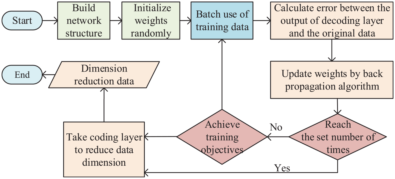
Flow chart of autoencoder feature dimension reduction.

The first step involves defining the network structure. The neural network structure can be implemented in PyTorch, a deep learning framework developed for scientific research. It has a useful modular function to quickly implement the design of the neural network. Use the sequential class in PyTorch to configure the parameters of each layer from top to bottom, and create the encoder and decoder, respectively. The output of the encoder is used as the input to the decoder. Set the input layer to linear and the number of units to 248, identical to the number of dimensions of the data. The hidden layer is set to sigmoid and the number of units can be adjusted; the output layer is linear and its number of units is also fixed at 248.

The second step features the initialization of the parameters. When the input data are unchanged, all parameters are updated from zero. Because the weights are computed through back propagation errors, the same training results are obtained regardless of the order of the data input. Therefore, it is necessary to assign initial values to all parameters at the beginning of training that obeys a normal distribution, and the size of ò can be adjusted; it is usually set to 0.01. After each initialization, record the seed that generates a random number and use it to obtain the same initial network parameters.

The third step involves training the model. Stochastic gradient descent is used for training, and the mini-batch training method is adopted. Each batch uses four samples to update the parameters as well as a varying learning rate to avoid falling into the local optimum.

The loss function of the autoencoder is defined as the reconstruction error.³⁴ Assuming that the input is $x$ and the reconstruction result of is $z$ , the solution can be set as

L (x, z) = - \sum_{i = 1}^{n} [x_{i} \log z_{i} + (1 - x_{i}) \log (1 - z_{i})]

(3)

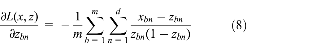
The batch training method is used to update the model, and the loss function is thus expressed as

L (x, z) = - \frac{1}{m} \sum_{b = 1}^{m} \sum_{n = 1}^{d} (x_{bn} \log (z_{bn}) + (1 - x_{bn}) \log (1 - z_{bn}))

(4)

where $m$ is the number of samples in each batch and $m$ is set to 4 here, $d$ is the total number of samples, and $x_{bn}$ and $z_{bn}$ represent the input and the output, respectively. The relationships between the parameters of each layer are as follows

\begin{array}{l} V_{i}^{(2)} = \sum_{n = 1}^{d} W_{m}^{(2)} x_{b n} + b_{i}^{(2)} \\ A_{i}^{(2)} = s (V_{i}^{(2)}) \\ V_{j}^{(3)} = \sum_{i = 1}^{h} W_{i j}^{(3)} A_{i}^{(2)} \\ A_{j}^{(3)} = s (V_{j}^{(3)}) \end{array}

(5)

Then, the output corresponding to the sample is

\begin{matrix} z_{bn} = A_{j}^{(3)} = s (\sum_{i = 1}^{h} W_{ij}^{(3)} s (V_{j}^{(2)}) + b_{j}^{(3)}) \\ = s (\sum_{i = 1}^{h} W_{ij}^{(3)} s (\sum_{i = 1}^{h} W_{ni}^{(2)} x_{bn} + b_{i}^{(2)}) + b_{j}^{(3)}) \end{matrix}

(6)

$V$ is the input value and $A$ is the excitation value corresponding to each layer. According to the chain rule, the derivative of the loss function is calculated with respect to each parameter

\begin{matrix} \frac{\partial L (x, z)}{\partial W_{ni}^{(2)}} & = \frac{\partial L (x, z)}{\partial z_{bn}} \frac{\partial z_{bn}}{\partial W_{ni}^{(2)}} \\ \frac{\partial L (x, z)}{\partial b_{i}^{(2)}} & = \frac{\partial L (x, z)}{\partial z_{bn}} \frac{\partial z_{bn}}{\partial b_{i}^{(2)}} \\ \frac{\partial L (x, z)}{\partial b_{j}^{(2)}} & = \frac{\partial L (x, z)}{\partial z_{bn}} \frac{\partial z_{bn}}{\partial b_{j}^{(2)}} \end{matrix}

(7)

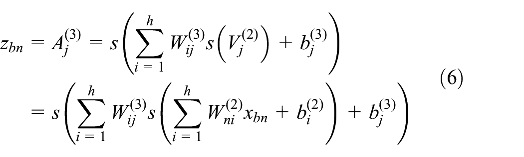
The derivative of the loss function in formula 7, with respect to $z_{bn}$ , is

\frac{\partial L (x, z)}{\partial z_{bn}} = - \frac{1}{m} \sum_{b = 1}^{m} \sum_{n = 1}^{d} \frac{x_{bn} - z_{bn}}{z_{bn} (1 - z_{bn})}

(8)

The model parameters are updated according to the above steps until the loss function no longer decreases. When the loss function does not change after 50 consecutive iterations, the training is stopped.

The fourth step consists of FS. Once model training has been completed, use the encoder to process all the data and obtain compressed data as the output. In addition, the relative importance of each feature is obtained through the weight of each feature of the input layer after training.

Improved GBDT model based on resampling strategy

Analysis of the impact of unbalanced samples on GBDT model

The amount of abnormal data in the network environment is far less than the normal traffic, which will lead to an extreme data imbalance. In this case, most algorithms learn a large number of samples of a certain type, while ignoring the classification accuracy of the other samples. Especially in the GBDT algorithm, data imbalance will affect the splitting of the tree nodes. Due to an insufficient number of samples, there are fewer nodes in the subtree, which cannot form an effective classification structure.³⁵

According to formula 4, when the parameters are updated, it is not the actual loss function, but its approximate expression is used to solve the gradient. The approximate expression is the sum of losses in all samples. Therefore, even if a certain gradient direction has a great loss reduction to a few classes, if the loss reduction of most classes of samples is smaller than that of other directions, it will not be the optimal gradient after final summation due to the number of reasons. At this time, most samples play an important role in the optimization process, which weakens the influence of a few samples on the algorithm.

On the contrary, the GBDT algorithm draws on the idea of generating a bootstrap subtraining set of random forest. For unbalanced data, the subtree training set obtained by this method encounters the same problem of imbalance as the original set. According to the splitting criterion used in the tree algorithm, the splitting index is related to the respective ratios of different types of samples.³⁶ To prevent over-fitting in the training process, node splitting can be performed only when the judgment index is greater than a set threshold. When the sample is extremely unbalanced, the value of this index is very small and new nodes cannot be correctly generated.

On the whole, when the data are unbalanced, the algorithm cannot learn sample-related information. This leads to the model having a good classification effect for the majority class but a poor one for the minority class of samples. This article proposes an integrated T-RBSMOTE algorithm to improve the training process of the GBDT algorithm.

Integrated T-RBSMOTE sampling

The integrated T-RBSMOTE sampling is used in the training process of the GBDT algorithm. The main steps are shown in Figure 8. Once the training set for each subtree has been obtained through random sampling, the ratio of abnormal samples is calculated. If the threshold of this ratio is reached, proceed directly to the next step; if the ratio is lower than the threshold, continue to randomly select abnormal samples from the original sample set and add them until the desired ratio is reached. Following this, a target ratio is set, the Tomek-links algorithm is used to delete the majority class of samples, redundant samples in the training set are eliminated, and Borderline-SMOTE is used to simulate and synthesize the abnormal samples. In view of the strong imbalance in data on botnet traffic, the required resampling ratio is also high. If the original sample is directly used for resampling, repeated synthetic samples may be generated. Therefore, by recursively using the Borderline-SMOTE algorithm, the generated sample is added to the original set once its size is twice that of the original sample, and sample synthesis is continued. The process stops when the sample ratio of the subtraining set reaches the target value. This recursive resampling helps avoid the repeated use of samples, guarantees the diversity of the subtrees, and makes the ratio of abnormal data more reasonable and stable such that each subtree can learn enough sample-related information.

Figure 8.

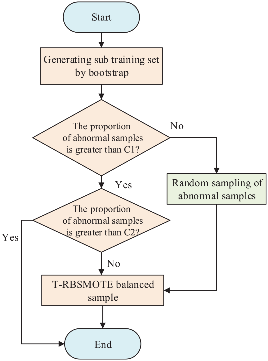
T-RBSMOTE resampling flow chart.

Experimental results and analysis

In this section, we present our results in evaluating the presented botnet detection approach.

Datasets and tools

This article uses the public ISCX-botnet dataset³⁷ to study the botnet detection algorithm. This dataset contains data collected in two intervals. Each dataset contained the original data packets of normal traffic and botnet communication. The difference was that a new type of sample was added to the latter part of the data. The ratios of various samples in the dataset are shown in Table 2. The ratio of the number of normal samples to that of abnormal samples was greater than 10:1, implying a significant imbalance.³⁸

Table 2.

Different sample proportion.

Category	Number	Proportion (%)
Normal data	310,526	94.18
Neris	5167	1.57
Rbot	2757	0.84
Internet Relay Chat	8942	2.71
Virut	2341	0.71
Total	329,733	100.00

The experimental program code of the botnet detection algorithm was written in Python. Experiments are conducted on a MacBook 2018, and the libraries and related functions used in our experiment are shown in Table 3.

Table 3.

Tool library list.

Library name	Function
Sklearn	Algorithm interface and data processing
Numy	Matrix operation, statistics of experimentalresults
Pandas	Access and arrangement of dataset
PyTorch	Construction of neural network model
Seaborn	Demonstration of experimental results

Evaluation rules

The confusion matrix is generated according to the correctness of the results of classification, which is shown in Table 4.³⁹ Each item in the matrix represents the number of results in the corresponding scenario. Given a category, we can determine whether a sample belonged to it according to its label. If it did, its value is set to one or positive, and is otherwise set to zero or negative. The algorithmic model obtained by training could also be used to determine whether a given sample is positive or negative. If the judgment value is identical to the true value of the sample, the result of the judgment is true, and is otherwise false.

Table 4.

Confusion matrix.

	Judged value
	Positive	Negative
True value
Positive	TP	FN
Negative	FP	TN

TP: true positive; FN: false negative; FP: false positive; TN: true negative.

The classification results of the algorithm can be divided into four cases:

True positive (TP): The true value was positive, as was the judged value.

True negative (TN): The true value was negative, as was the judged value.

False negative (FN): The true value was positive but the judged value was negative.

False positive (FP): The true value was negative but and the judged value was positive.

We assess the proposed detection methods in terms of accuracy, recall, precision, F-measure, and stability. These evaluation rules are given by

Accuracy = \frac{TP + TN}{TP + TN + FP + FN}

(9a)

Recall = \frac{TP}{TP + FN}

(9b)

Precision = \frac{TP}{TP + FP}

(9c)

F_{measure} = \frac{(α^{2} + 1) \Pr \cdot Re}{α^{2} (\Pr + Re)}

(9d)

In Formula 9d, $α$ is usually taken as one, and is called the F1-measure. It combines recall and precision, and can be used to comprehensively evaluate the classification results of certain types of data obtained by the algorithm. We also used two other evaluation indicators, the receiver operating characteristic (ROC) curve and stability. The ROC curve was originally used for signal detection, and was later introduced to ML to evaluate model performance in terms of classification. It is an important method of statistical analysis. The ROC curve can be formed by taking the FP rate under different judgment thresholds as the abscissa and the TP rate as the ordinate, and the area under the curve (AUC) can then help quantify and evaluate the classification effect of the model. The stability of the algorithm refers to whether the model can maintain good classification effect when the samples are altered.⁴⁰ In light of the variability of the network environment, the appearance of new data, and high frequency of changes to the data, high stability can help reduce the failure rate of the model over a short period, the frequency of update, and the cost of maintenance. No universal quantitative index is available to assess the stability of algorithms. In this article, the classification results are tested by using data collected in different periods, and stability is evaluated according to changes in the results.

Experiment on data feature optimization

Preferences

In the training process, we not only get the parameters such as weight and deviation but also use a series of artificial preset parameters in various learning models, which are called superparameters. Superparameters that can be set in the autoencoder include the number of hidden layer units and coding layers. One, three, and five hidden layers are used to train the network, and the convergence performance and reconstruction error are recorded after the training process, as shown in Figure 9.

Figure 9.

Comparison of reconstruction error curves of different layers.

Figure 9 shows that the three-hidden layer structure converges fastest with the smallest reconstruction error, while the five-hidden layer structure converges slowest with the largest reconstruction error. Therefore, we did not consider using a deeper network structure.

After analyzing the experiment with FS algorithm, a total of 10 feature dimensions were retained because the final number of data dimensions could not be less than 10. The number of coding units ranges from 11 to 15. According to a comparison of reconstruction error curves in Figure 10, it is obvious that the number of coding units has little effect on the reconstruction error. Considering the need to reduce the number of feature dimensions, 11 layers of coding units are determined to be the best choice.

Figure 10.

Comparison of reconstruction error curves of different layers.

According to the above results, a network structure with three hidden layers and 11 units in the coding layer is used in subsequent experiments to reduce the number of dimensions of the features, that is, the optimized number of feature dimensions is 11.

Comparison of FS methods

The 20 most effective features are obtained using the weight of each feature of the input layer, as shown in Table 5. It is evident that port-related information is an important basis for judgment. Most of the other statistical features are influential, which shows that the features obtained by statistical analysis are effective.

Table 5.

Names and meanings of the top 20 important features.

ID	Name	Meaning
1	dstport	Destination port
2	srcport	Source port
208	var_data_ip	Packet byte variance
4	q1_IAT	Interquartile of arrival interval
72	mean_IAT	Average arrival interval
84	min_segm_size_b a	Opposite minimum packet
3	min_IAT	Minimum arrival interval
16	var_IAT	Arrival interval variance
5	med_IAT	Median arrival interval
98	initial_window_packtes_a b	Number of opposite packets in initial time window
183	med_dat_ip_b a	Median number of bytes in opposite packets
79	mss_requested_a b	Number of packets containing MSS requests
97	initial_window_packets_b a	The number of packets sent in the initial time window
73	sacks_sent_a b	ACK packet containing sack information
7	q3_IAT	Interarrival 3/4 quantile
99	ttl_stream_length_a b	Average TTL of forward traffic
215	idle	Idle state duration
82	max_segm_size_b a	Opposite maximum packet
14	sacks_sent_a b	ACK packet containing sack information
6	mean_IAT	Average arrival interval

The principal component analysis (PCA), kernel principal component analysis (KPCA),⁴¹ random addition and deletion FS, and the method in this article are used to reduce the dimension of features, and then the GBDT model is trained by the feature data, and the classification accuracy is compared. To avoid random interference, a total of 30 experiments have been carried out. The comparison results are shown in Table 6. Each method finally obtains 10 or 11 features, indicating that they contain most of the information.

Table 6.

Comparison of different feature selection methods.

Contrast item	Principal component analysis	Kernel principal component analysis	Subset search	Autoencoder
Characteristic number	10	11	11	11
Classification accuracy	87.31%	94.30%	92.67%	94.32%
Running time/min	7	33	52	10

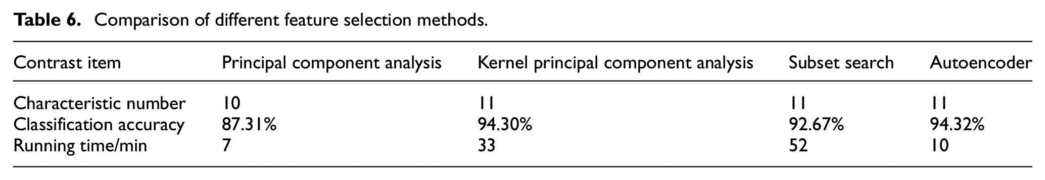
The first 10 features obtained by PCA, KPCA, and FS are shown in Table 7. It is clear that 80% of the important features overlapped with those obtained by the proposed method. This shows its usefulness for FS. By contrast, the features obtained by simple PCA could not guarantee accuracy, whereas the accuracies of feature screening and KPCA were higher, but they required longer calculation times. Compared with the two models, the model trained by features obtained using the proposed method had slightly higher classification accuracy and shorter calculation time. The neural network model thus obtained could be further updated afterward, which is suitable for anomaly detection.

Table 7.

The important characteristics obtained by other methods are analyzed.

Algorithm	Important features ID
PCA	1 2 72 84 95 98 97 16 105 108
KPCA	1 2 4 5 208 16 3 84 97 73
FS	1 2 97 98 72 84 106 96 14 3

PCA: principal component analysis; KPCA: kernel principal component analysis; FS: feature selection.

Experiment on classification algorithm

The main steps of this experiment were as follows:

According to the information on IP addresses, labeling the processed data categories to form a dataset, and divide it into a training set, a verification set, and a test set. Each dataset is used for model training, optimization, and testing.

The training set is used for unsupervised training of neural network of automatic encoder. The network obtained in this way is used to reduce the dimension of data, and they are input into the learning algorithm to train it. According to the characteristics of data and categories, the subtree is trained, and finally, the required classification model is obtained.

Evaluating the performance, adjusting the structure of neural network and parameters of GBDT model by cross-validation method to meet the target requirements, and storing the learned model.

Preliminary comparison experiment

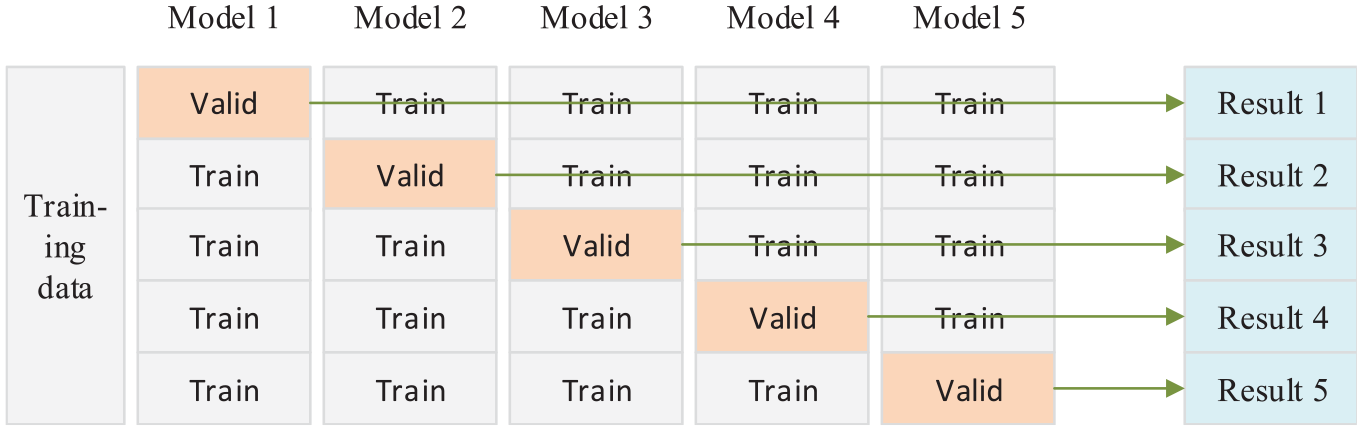
We carried out a preliminary comparative experiment on various algorithms and chose the best algorithm. Compared algorithms include NB, DT, SVM, k-nearest neighbor (KNN), and the improved GBDT algorithm proposed in this article. The first part of ISCX-botnet dataset is divided into a training set and a test set. The training set is used to train and optimize the model, and the test set is used to test its classification effect. The training set is used to construct the model using five-fold cross-validation, and the process of verification is shown in Figure 11. The training data are divided into five groups, and 20% of the data from each are used as the verification data. The other 80% of the data are used as the training set. A total of five groups of models and test results are obtained. If the group accuracy is not much different, the model with the best effect is selected. Then, we use the divided test set and the second part of ISCX-bot data to evaluate the effect of the model. The second part of the data is only used to test the stability of the algorithm to sample changes.

Figure 11.

Cross-validation process.

To ensure the objectivity of the results of comparison, all data are processed in the same manner, and the hyperparameters of each algorithm are set to commonly used default values. The index used for comparison is the classification accuracy of each algorithm. The results are shown in Figure 12. The training times of the algorithms are compared when the sample sizes are 300,000; 400,000; and 500,000, as shown in Figure 13.

Figure 12.

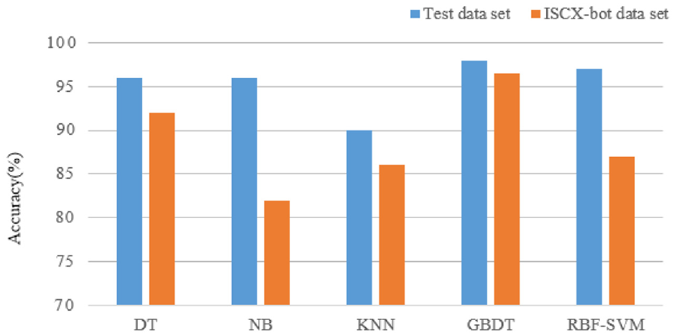
A comparison of accuracy of different algorithms.

Figure 13.

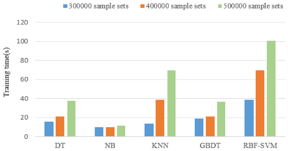
A comparison of training time of different algorithms.

The accuracy of GBDT records is very high; when the data changed, it maintains a good classification effect, and is stable. At the same time, its running time is shorter, even in case of changes in sample size. When the amount of data is large, it is faster than the other algorithms tested. According to these results, the GBDT algorithm has comprehensive advantages in terms of stability, accuracy, and the processing of large amounts of data. Therefore, it can better classify network traffic.

Optimizing hyperparameters of GBDT model

The principle of the GBDT algorithm is complex, and it includes many artificially set parameters. The main parameters include the learning rate $η$ , number of subtrees $T$ , depth of the tree structure, and the number of leaf nodes. The number of subtrees and the learning rate have a greater impact on model performance than the other parameters. Excluding special cases, they are generally not adjusted.⁴² To study the influence of the number of subtrees $T$ and the learning rate $η$ on the performance of the algorithm, the former was set to 50 equal values between 10 and 500 and the latter was set to 50 equal values between 0.01 and 0.5. We used 2500 sets of hyperparameter values to train the model and compare its performance using different parameters. In the experiment, we used 10% of the samples as the test set and the remaining as the training set. Five-fold cross-validation was used for training. The average value of the indices obtained in five models was taken as the result. Changes in the performance of the model with the number of subtrees and the learning rate are shown in Figure 14.

Figure 14.

Accuracy and F1-measure’s variation chart about parameters. (a) Thermal chart of accuracy change. (b) Thermal chart of F1-measure change.

Figure 14 compares the overall accuracy and the geometric mean value of the F1-measure with changes in the parameters. It is evident that the parameter setting had little effect on accuracy, while the F1-measure was more significantly affected by it. This is because of the unreasonable parameter setting that caused the F1-measure of some categories of the algorithm to decrease, which affected the overall index. The algorithm maintained a good classification effect for normal samples that accounted for more than 90% of all samples. Therefore, its overall accuracy did not change by much. The experimental results show that when the learning rate was less than 0.05 or the number of subtrees was greater than 300, the performance of the algorithm did not change significantly. That is to say, the combination of these two parameters can simultaneously guarantee higher training efficiency and better classification performance. Thus, the most suitable parameters are $η = 0.05$ , $T = 300$ .

Analysis and comparison of resampling methods

The benchmark resampling methods ROS, RUS, and SMOTE-Tomek⁴³ are used on the two-dimensional sample data, and the sample ratio reaches 5:1. Comparison of the results leads to the change of sample distribution and classification boundary, as shown in Figure 15, where the red represents the majority class of samples.

Figure 15.

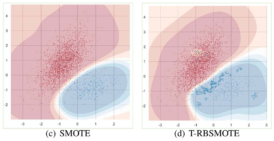
The change of decision boundary for two-dimensional sample data classification. (a) Original sample. (b) Tomek-Links. (c) SMOTE. (d) T-RBSMOTE.

Following SMOTE sampling, the classification boundary changed, and index of the results of classification of the algorithm improved. However, owing to the random selection of the sampling points, data repeatability was high. Tomek was used to reduce the sample density of the majority class, but the number of samples that could be deleted was limited. Thus, this did not have a significant impact on the classification model. The T-RBSMOTE algorithm resampled data only at the boundary points. We trained the new GBDT for classification and compared it with the original data, from which it is clear that the classification boundary shifted to the majority class such that more samples of the minority class were correctly divided.

We further explored the impact of resampling on the GBDT algorithm and analyzed changes in the number of subtree nodes during the experiment. The average numbers of nodes updated in 30 iterations using different resampling methods are shown in Figure 16.

Figure 16.

Influence of different resampling strategies on the number of leaf nodes.

The use of Tomek-Links alone yielded almost no change in the number of nodes, whereas using SMOTE and T-RBSMOTE significantly increased the average number of nodes in the subtree. The impact of T-RBSMOTE was more significant, and the final number of average nodes changed from 11 to 26. This shows that when the minority classes were oversampled, the tree algorithm learned more sample-related information to form a more effective branch structure. The T-RBDMOTE algorithm used here thus achieved better results. We then used the test data to evaluate the classification performance of the model. We compared the performance of the GBDT model trained using the original samples with that when it was trained using different reconstruction samples. The recall rate, accuracy, and F1-measure of each category were compared as shown in Figure 17. It shows the performance of Tomek-Links, SMOTE, and T-RBSMOTE from left to right on the original data. The corresponding index values continued to increase. The changes in color show that the good ability of the model to identify normal traffic was maintained, and its detection of other categories significantly improved.

Figure 17.

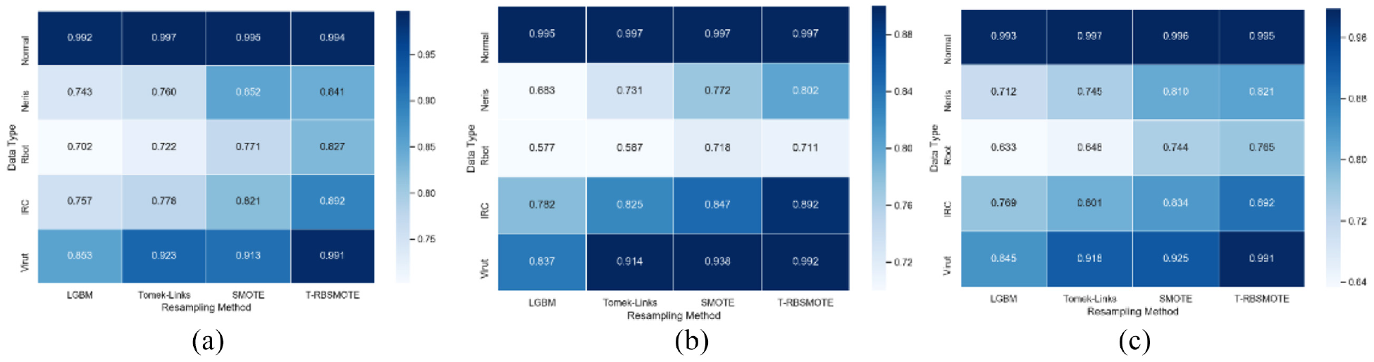
Effect comparison of GBDT model before and after resampling. (a) Recall. (b) Accuracy. (c) F1-measure.

A comparison of the ROC curves of the model before and after resampling is shown in Figure 18. The curve of each category becomes steeper, and the AUC is 0.99. This means that the model could simultaneously maintain a low false alarm rate and a high recognition rate. The overall accuracy also increases from 95.2% to 99.2%. The above results show that the proposed resampling algorithm can solve the problem of data imbalance and improve the performance of the trained model.

Figure 18.

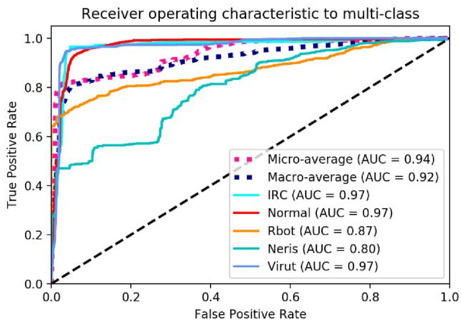
Comparison of ROC curves before and after resampling.

Conclusion and future work

This article proposed a novel botnet detection method for unbalanced traffic data in the communication network of smart systems, based on an autoencoder neural network in cooperation with DTs. The autoencoder neural network was used to optimize the characteristics of the traffic data, which can help accurately discover botnet activities. To overcome the shortcomings of existing feature dimension reduction methods, a feature dimension reduction method based on autoencoder neural network was proposed. To solve the problem of unbalanced traffic data samples, a GBDT training strategy T-RBSMOTE based on resampling was proposed to eliminate noise and reduce over-fitting. Simulation synthesis is used to make up for the shortage of abnormal samples and lack of information, increase the number of branches of tree nodes, and improve the classification effect. Finally, the results of experiments on the ISCX-botnet traffic dataset show that the proposed method achieved better botnet detection performance with 99.10% recall, 99.20% accuracy, 99.1% F1 score, and 99.0% AUC. The proposed resampling algorithm can solve the problem of data imbalance and improve the performance of the trained model. The limitation of this article focuses on offline traffic data, and does not consider the dynamic nature of traffic. For our future work, we will design a real-time online detection method based on different deep learning models to detect malicious network threats such as DDoS attacks.

Footnotes

Handling Editor: Peio Lopez Iturri

Author Note

Li Duan, is now affiliated to State Key of Laboratory of Networking and Switching Technology, Beijing University of Posts and Telcommunications,100876, China.

Declaration of conflicting interests

The author(s) declared no potential conflicts of interest with respect to the research, authorship, and/or publication of this article.

Funding

The author(s) disclosed receipt of the following financial support for the research, authorship, and/or publication of this article: This research was supported by the National Natural Science Foundation of China (No.61902021), Beijing Natural Science Foundation Municipality (No.4212008), Open Foundation of State key Laboratory of Networking and Switching Technology (Beijing University of Posts and Telecommunications) under Grant SKLNST-2019-2-08, the Project of Civil aviation safety capacity under No. PESA2019074, and the fundamental research funds for the central universities under No. 3122018C036.

Data availability

A data availability statement is compulsory for research articles and clinical trials. Here, authors must describe how readers can access the data underlying the findings of the study, giving links to online repositories and providing deposition codes where applicable. For more information on how to compose a data availability statement, including template examples, please visit .

References

Hao

Liu

Baldi

, et al. Unsupervised detection of botnet activities using frequent pattern tree mining. Complex Intell Syst. Epub ahead of print 25 February 2021. DOI: 10.1007/s40747-021-00281-5.

Wazid

Das

Rodrigues

JJPC

, et al. IoMT malware detection approaches: analysis and research challenges. IEEE Access 2019; 7: 182459–182476.

Vishwakarma

Jain

AK.

A survey of DDoS attacking techniques and defence mechanisms in the IoT network. Telecommun Syst 2020; 73(1): 3–25.

Catania

Garino

. Automatic network intrusion detection: current techniques and open issues. Comput Electr Eng 2012; 38(5): 1062–1072.

FireHOL. All cybercrime IP feeds, http://iplists.firehol.org (accessed 15 December 2020).

Proofpoint. Emerging threats open snort ruleset, http://www.emergingthreats.net/ (accessed 15 December 2020).

Alauthaman

Aslam

Zhang

, et al. A P2P Botnet detection scheme based on decision tree and adaptive multilayer neural networks. Neural Comput Appl 2018; 29(11): 991–1004.

Bou-Harb

Debbabi

Assi

. Big data behavioral analytics meet graph theory: on effective botnet takedowns. IEEE Netw 2016; 31(1): 18–26.

Kudo

Kimura

Inoue

, et al. Behavior analysis of self-evolving botnets. In: International conference on computer, information and telecommunication systems (CITS), Kunming, China, 6–8 July 2016, pp.1–5. New York: IEEE.

10.

Mousavi

Khansari

Rahmani

. A fully scalable big data framework for Botnet detection based on network traffic analysis. Inform Sci 2020; 512: 629–640.

11.

Saad

Issa Traor Ghorbani

Sayed

, et al. Detecting P2P botnets through network behavior analysis and machine learning. In: Proceedings of the ninth annual international conference on privacy, security and trust, Montreal, QC, Canada, 19–21 July 2011, pp.300–317. New York: IEEE.

12.

Yin

Ghorbani

. P2P botnet detection based on association between common network behaviors and host behaviors. In: International conference on multimedia technology, Hangzhou, China, 26–28 July 2011, pp.5010–5012. New York: IEEE.

13.

Garcia

. Learning from imbalanced data. IEEE Trans Knowl Data Eng 2009; 21(9): 1263–1284.

14.

Panimalar

Rameshkumar

. A novel traffic analysis model for botnet discovery in dynamic network. Arab J Sci Eng 2019; 44: 3033–3042.

15.

Abdurrahman

Tankut

. Deep learning to detect botnet via network flow summaries. Neural Comput Appl 2019; 31(11): 8021–8033.

16.

Haddadi

Zincir-Heywood

. Botnet behaviour analysis: how would a data analytics-based system with minimum a priori information perform? Int J Netw Manag 2017; 27(4): e1977.

17.

Drasar

Vizvary

Vykopal

. Similarity as a central approach to flow-based anomaly detection. Int J Netw Manag 2014; 24(4): 318–336.

18.

Stevanovic

Pedersen

. An efficient flow-based botnet detection using supervised machine learning. In: International conference on computing, networking and communications (ICNC), Honolulu, HI, 3–6 February 2014, pp.797–801. New York: IEEE.

19.

Chen

Niu

Zhang

, et al. An effective conversation-based botnet detection method. Math Probl Eng 2017; 1: 1–9.

20.

Kirubavathi

Anitha

. Botnet detection via mining of traffic flow characteristics. Comput Electr Eng 2016; 50: 91–101.

21.

Nogueira

Salvador

Blessa

. A botnet detection system based on neural networks. In: Proceedings of the fifth international conference on digital telecommunications (ICDT), Athens, 13–19 June 2010, pp.57–62. New York: IEEE.

22.

Salvador

Nogueira

Franca

, et al. Framework for zombie detection using neural networks. In: Proceedings of the fourth international conference on internet monitoring and protection (ICIMP), Venice, 24–28 May 2009, pp.14–20. New York: IEEE.

23.

Sheikhan

Jadidi

. Flow-based anomaly detection in high-speed links using modified GSA-optimized neural network. Neural Comput Appl 2014; 24(3): 599–611.

24.

Livadas

Walsh

Lapsley

, et al. Using machine learning techniques to identify botnet traffic. In: 2006 31st IEEE conference on local computer networks, Tampa, FL, 14–16 November 2006, pp.967–974. New York: IEEE.

25.

McKay

Pendleton

Britt

, et al. Machine learning algorithms on botnet traffic: ensemble and simple algorithms. In: Proceedings of the 2019 3rd international conference on compute and data analysis, University of Hawaii Maui College, USA, 14–17 March 2019, pp.31–35. New York: Association for Computing Machinery.

26.

Gahelot

Dayal

. Flow based botnet traffic detection using machine learning. In: Singh

Panigrahi

Suryadevara

, et al. (eds) Proceedings of ICETIT 2019. Cham: Springer, 2020, pp.418–426.

27.

Vincent

Larochelle

Lajoie

, et al. Stacked denoising autoencoders: learning useful representations in a deep network with a local denoising criterion. J Mach Learn Res 2010; 11(12): 3371–3408.

28.

Ding

Zhu

Wei

. Traffic identification of mobile apps based on variational autoencoder network. In: Proceedings of international conference on computational intelligence and security (CIS), Hong Kong, China, 15–18 December 2017, pp.1135–1143. New York: IEEE.

29.

. Probabilistic boosting-tree: learning discriminative models for classification, recognition, and clustering. In: IEEE international conference on computer vision (ICCV’05) volume 1, Beijing, China, 17–21 October 2005, pp.1589–1596. New York: IEEE.

30.

Yao

Chen

, et al. Inspection of exterior substance on high-speed train bottom based on improved deep learning method. Measurement 2020; 163: 108013.

31.

Lai

Ali

Hossain

, et al. Performance modeling and analysis of TCP and UDP flows over software defined networks. J Netw Comput Appl 2019; 130: 76–88.

32.

Moore

Zuev

. Internet traffic classification using Bayesian analysis techniques. In: Proceedings of the 2005 ACM SIGMETRICS international conference on Measurement and modeling of computer systems, Banff, Alberta, Canada, 6–10 June 2005, pp.50–60. New York: Association for Computing Machinery.

33.

Zhou

Huang

. Deep learning detection based on traffic characteristics of botnet. Inform Techn 2018; 4: 1–9.

34.

. Building high-level features using large scale unsupervised learning. In: IEEE international conference on acoustics, speech and signal processing, Shanghai, China, 20–25 March 2016, pp.8595–8598. New York: IEEE.

35.

Frnkranz

Gamberger

Lavrac

. Foundations of rule learning. Berlin: Springer Science & Business Media, 2012.

36.

Murphy

. Machine learning: a probabilistic perspective. Cambridge, MA: The MIT Press, 2012.

37.

Grill

Stiborek

Zunino

. An empirical comparison of botnet detection methods. Comp Secur 2014; 45: 100–123.

38.

Chawla

. Data mining for imbalanced datasets: an overview. In: Maimon

Rokach

(eds) Data mining and knowledge discovery handbook. Boston, MA: Springer, 2005, pp.853–867.

39.

Asadi

Jamali

MAJ

Parsa

, et al. Detecting botnet by using particle swarm optimization algorithm based on voting system. Future Gener Comput Syst 2020; 107: 95–111.

40.

Biau

. Analysis of a random forests model. J Mach Learn Res 2012; 13(1): 1063–1095.

41.

Lee

Mendis

Triebe

, et al. Monitoring of a machining process using kernel principal component analysis and kernel density estimation. J Intell Manuf 2020; 31(5): 1175–1189.

42.

Dopke

Fritsche

Pierdzioch

. Predicting recessions with boosted regression trees. Int J Forecast 2017; 33(4): 745–759.

43.

Guo

Liu

Chen

, et al. Improved SMOTE algorithm to deal with imbalanced activity classes in smart homes. Neural Process Lett 2019; 50(2): 1503–1526.

A novel and highly efficient botnet detection algorithm based on network traffic analysis of smart systems

Abstract

Keywords

Introduction

Related work

Background

Autoencoder model

The GBDT model

Overall design of botnet detection algorithm

Preprocessing flow data

Data grouping aggregation based on DFI analysis

Data stream feature extraction based on statistical analysis

Data cleaning and preprocessing

Flow FS based on autoencoder

Improved GBDT model based on resampling strategy

Analysis of the impact of unbalanced samples on GBDT model

Integrated T-RBSMOTE sampling

Experimental results and analysis

Datasets and tools

Evaluation rules

Experiment on data feature optimization

Preferences

Comparison of FS methods

Experiment on classification algorithm

Preliminary comparison experiment

Optimizing hyperparameters of GBDT model

Analysis and comparison of resampling methods

Conclusion and future work

Footnotes

Author Note

Declaration of conflicting interests

Funding

Data availability

References