Sage Journals: Discover world-class research

Abstract

One method to create a high-performance computer is to use parallel processing to connect multiple computers. The structure of the parallel processing system is represented as an interconnection network. Traditionally, the communication links that connect the nodes in the interconnection network use electricity. With the advent of optical communication, however, optical transpose interconnection system networks have emerged, which combine the advantages of electronic communication and optical communication. Optical transpose interconnection system networks use electronic communication for relatively short distances and optical communication for long distances. Regardless of whether the interconnection network uses electronic communication or optical communication, network cost is an important factor among the various measures used for the evaluation of networks. In this article, we first propose a novel optical transpose interconnection system–Petersen-star network with a small network cost and analyze its basic topological properties. Optical transpose interconnection system–Petersen-star network is an undirected graph where the factor graph is Petersen-star network. OTIS–PSN_n has the number of nodes 10²ⁿ, degree n+3, and diameter 6n − 1. Second, we compare the network cost between optical transpose interconnection system–Petersen-star network and other optical transpose interconnection system networks. Finally, we propose a routing algorithm with a time complexity of 6n − 1 and a one-to-all broadcasting algorithm with a time complexity of 2n − 1.

Keywords

Optical transpose interconnection system Petersen-star interconnection network network cost graph

Introduction

Computing performance largely depends on processor speed and memory capacity. Parallel processing, which connects multiple processors, has emerged because improvements in the physical performance of processors and memory have relatively slowed down in recent years. For an interconnection network, the connection structure of the parallel processing system is represented on a topology. The interconnection network is represented as a graph mapping the processors as nodes and the communication links that connect the processors as edges.¹

Designing a good interconnection network is the same as creating a good parallel processing system. The interconnection networks that have been reported so far can be largely classified into mesh, torus, hypercube, and start graph classes. The hypercube class has been commercialized as iPSC/2, iPSC/860, and n-CUBE/2; the mesh class as MasPar Intel Paragon, XP/S, Touchstone DELTA System, and Mosaic C; and the three-dimensional mesh class as Cray T3D, MIT’s J-Machine, and Tera Computer.²

In the systems mentioned in the preceding paragraph, electronic signals are transmitted along the communication links. After the emergence of optical communication, an optical transpose interconnection system (OTIS), which combines the advantages of both electronic communication and optical communication, was proposed by Marsden et al.³ The OTIS network is implemented using free-space optoelectronic technology. In terms of transmission speed, power consumption, and error rate, the breakeven point for optical communication occurs when the length of the communication link is less than 1 cm. However, the installation cost is inexpensive for electronic communication.⁴

In OTIS, n groups consisting of n nodes exist. Electronic links are used for connections between nodes in a group of relatively short distances, whereas optical links are used for connections between nodes existing in different groups. OTISs have a fast message transfer speed and low power consumption. The OTISs reported so far include OTIS-ops,⁵ OTIS-pops,⁵ OTIS-stack graph,⁵ OTIS-mesh,⁶ OTIS-torus,⁷ OTIS-hypercube,⁸ OTIS-star graph,⁹ OTIS-swapped network,¹⁰ OTIS-hyper hexa-cell,¹¹ OTIS-biswapped network (BSN)-Mesh,¹² BSN-Torus,¹³ BSN-MOT (mesh of tree),¹⁴ and BSN-hyper hexa-cell (HHC).¹⁵

In a graph, the number of edges connected to a certain node is called the degree of the node, and the number of edges existing on the shortest path between two different nodes is called the distance. The degree of the graph is the maximum value among the degrees of all nodes. The diameter of the graph is the maximum value among the distances between arbitrary nodes. An important measure for evaluating interconnection networks is network cost, which can be calculated as the degree × diameter. Because degree refers to the number of communication links, the hardware installation cost increases when the degree increases. The diameter represents the length of the message transfer path between two processors, and when the diameter increases, the message transfer time increases, thus affecting the software cost. Thus, network cost is an important measure for the evaluation of interconnection networks.¹⁶

In this article, we propose an optical transpose interconnection system–Petersen-star network (OTIS–PSN) designed using a Petersen-star network (PSN), which has a small network cost. Section “OTIS, Petersen graph, and PSN” describes the basic concept of OTIS, the Petersen graph, and the PSN. Section “OTIS–PSN” defines the OTIS–PSN, analyzes its basic properties, and compares the network cost with other OTIS networks. Section “Communication algorithm” presents the routing and broadcasting algorithms for OTIS–PSN. Finally, section “Conclusion” concludes this article.

OTIS, Petersen graph, and PSN

OTIS

A basic graph that constitutes OTIS is called a factor graph (hereinafter referred to as factor). An OTIS consists of n groups, and one group is the same as one factor. The processors inside a group are connected by electronic links called electronic edges (hereinafter referred to as e-edges). The processors in different groups are connected by optical links called optical edges (hereinafter referred to as o-edges).

OTIS networks are designed based on the OTIS rule (the p processor of the g group is connected to the g processor of the p group), which uses previously presented mesh, torus, hyper cube, and star graphs as factor graphs. Furthermore, the biswapped family is designed to double the OTIS network and modify an edge. Because OTISs outperform previously announced interconnection networks theoretically, they have garnered significant research interest in recent times.^14,17–21

The address of node p in group g is denoted by <g, p>. According to the OTIS rule, <g, p>, and <p, g> are connected. Node p uses the node address of the factor, and thus g also uses the node address of the factor because g is exchanged with p. For example, for OTIS-Q₂, in which the factor is a two-dimensional hypercube, the node address is represented as shown in Figure 1.

Figure 1.

OTIS-Q₂.⁸

In OTIS, the number of groups is exactly the same as the number of nodes of the factor. Suppose that the number of nodes in the factor is N. Then, the number of nodes in the OTIS is N². The number of nodes of OTIS-Q₂ in Figure 1 is 16 (=4²).

The outline of OTIS routing is as follows. The starting node is S = <g₁, p₁>, and the terminal node is T = <g₂, p₂>. The path using the e-edge is represented as →, and the path using o-edge as =>. If g₁ = g₂, then the routing between the two nodes follows the routing of the factor. If g₁≠g₂, then the routing path between the two nodes is

< g_{1}, p_{1} > \to < g_{1}, g_{2} > = > < g_{2}, g_{1} > \to < g_{2}, p_{2} >

Petersen graph

The Petersen graph consists of 10 nodes and 15 edges. It has the best network cost among graphs with 10 nodes, and has a degree of 3 with a diameter of 2. Figure 2 shows the Petersen graph. The number on the left in the node address is smaller than the number on the right.²²

Figure 2.

Petersen graph and spanning tree: (a) the Petersen graph and (b) spanning tree.²

In a Petersen graph, P = (Vp, Ep); Node Vp = xy; Edge Ep = (xy, x′y′); x, y ∈ {1,2,3,4,5}; and x′,y′ ∈ {{1,2,3,4,5} − {x, y}}. It is assumed that in the Petersen graph, node u = u₁u₂ is the start node and node v = v₁v₂ is the destination node. Node w is composed of {1,2,3,4,5} − {{u₁, u₂} ⋃ {v₁, v₂}}. The routing algorithm from u to v is shown in Algorithm 1.²

Algorithm 1.

Routing (u, v) {
1: if {u₁, u₂} ⋂ {v₁, v₂} = ∅2: u → v;3: elseu → w → v;4:}

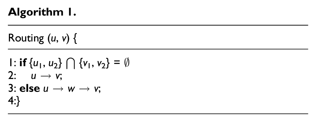
For the all-port model, the one-to-all broadcasting in the Petersen graph is edge-disjoint and broadcasting time is 2. Initially, node 12 has a message. As presented in Figure 2(b), the broadcasting algorithm given in Algorithm 2 is applied.

Algorithm 2.

Broadcasting {
1: Node 12 sends a message to its child nodes, 34, 35, and 45;2: Nodes 34, 35, and 45 send the received messages to their respective child nodes.3:}

Because the Petersen graph is a node (edge)-symmetric graph, Algorithm 2 is valid even though any arbitrary node can have a message initially.

PSN

The PSN uses the Petersen graph as the basic module. The number of internal edges that are connected to one node is three and the number of external edges is n − 1. PSN_n is a graph with 10ⁿ as the number of nodes, n+2 as the degree, and 3n − 1 as the diameter.²³

PSN_n = (Vp, Ep). The node of PSN_n is defined below

\begin{matrix} Vp = {p_{1} p_{2} p_{3} \dots p_{i - 1} p_{i} p_{i + 1} \dots p_{2 n - 1} p_{2 n} | (p_{i} p_{i + 1}, i is odd) \\ is the node address of the Petersen graph \end{matrix}}

The edges of PSN_n can be divided into internal and external edges. The internal edges connect nodes belonging to the same Petersen graph. The external edges connect nodes belonging to different Petersen graph. An external edge connects two nodes that have exchanged the symbols of p₁p₂ and p_ip_i₊₁ of the node addresses with each other. The external edge of PSN_n is defined below

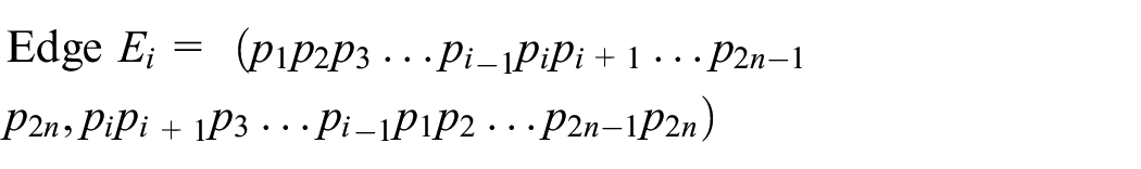
\begin{matrix} Edge E_{i} = (p_{1} p_{2} p_{3} \dots {p_{i}}_{- 1} p_{i} p_{i + 1} \dots p_{2 n - 1} \\ p_{2 n}, p_{i} {p_{i}}_{+ 1} p_{3} \dots {p_{i}}_{- 1} p_{1} p_{2} \dots p_{2 n - 1} p_{2 n} \end{matrix})

where 2 < i < 2n and i is odd.

In Figure 3, the numbers in black are p₁p₂ and the numbers in red are p₃p₄. For example, nodes 1245 and 1234 are connected to nodes 4512 and 3412, respectively, through external edges. In Figure 3, the external edges are indicated by blue solid lines, and the internal edges are indicated by black solid lines.

Figure 3.

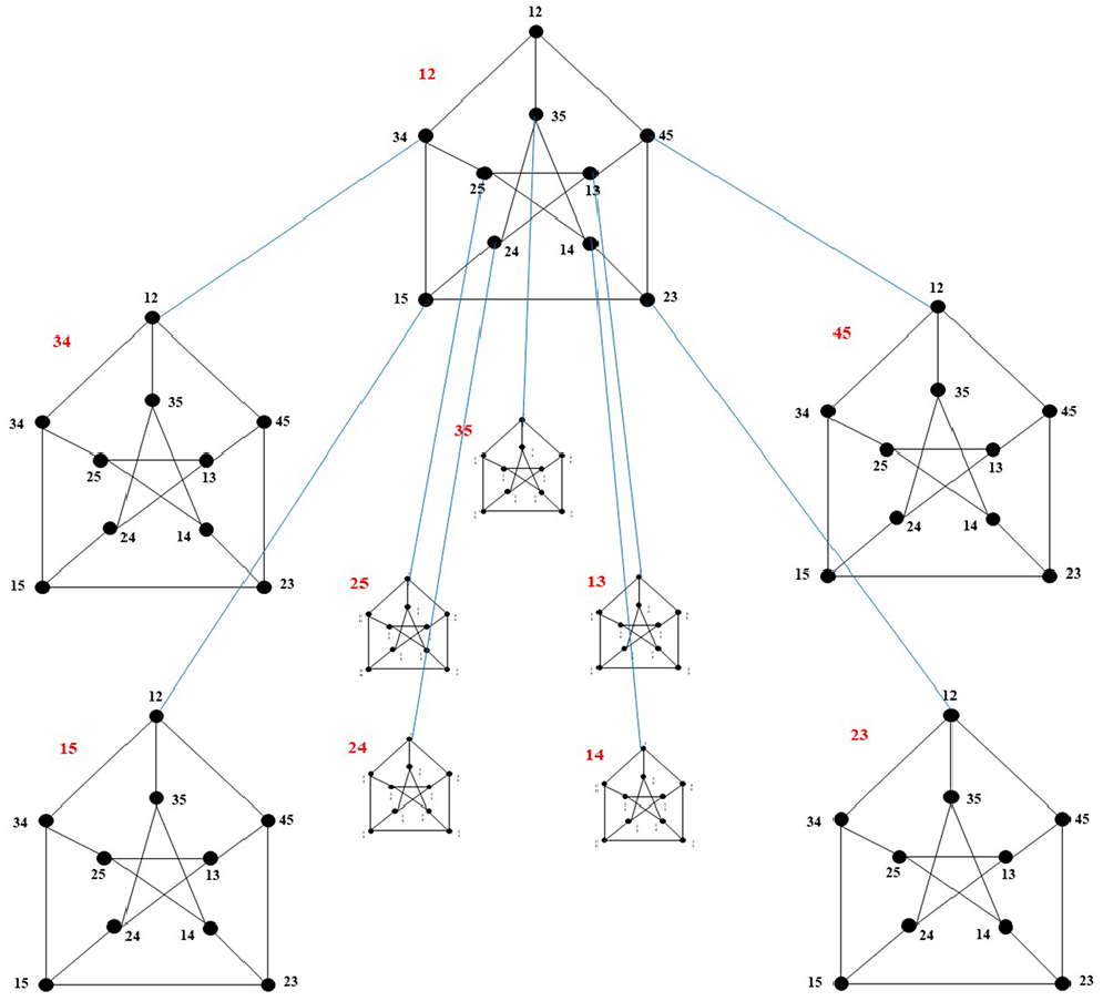
Two-level Petersen-star PSN₂.²³

It is assumed that in PSN_n, node u = u₁u₂u₃…u_i_− 1u_iu_i₊₁…u_2n − 1u_2n is the start node and node v = v₁v₂v₃…v_i_− 1v_iv_i₊₁…v_2n − 1v_2n is the destination node. The routing algorithm from u to v is as given in Algorithm 3.²³

Algorithm 3.

Routing (u, v) {
1: for i = 2n to 4 step –2 {2: u₁u₂ is changed to v_2i − 1v_2i; by Algorithm 1.3: u₁u₂ and u_2i − 1u_2i exchanged; by external edge E_2i − 1.4: }5: u₁u₂ is changed to v₁v₂; by Algorithm 1.6:}

The time complexity of Algorithm 3 is as follows. In terms of the worst case in each line, the time complexity is 2 in lines 2 and 5, and 1 in line 3. Therefore, the time complexity is (n − 1) × (2+1)+2 = 3n − 1. This value is the diameter of PSN_n. For example, if u = 12341345 and v = 35241525 in PSN₄, the routing path is as follows

\begin{matrix} (u) 12341345 \to 25341345 \to 45341325 \to 15341325 \\ \to 15341325 \to 13341525 \to 24341525 \\ \to 34241525 \to (v) 35241525 \end{matrix}

OTIS–PSN

Definition

OTIS–PSN_n is divided into 10ⁿ groups, where each group has 10ⁿ nodes. OTIS–PSN_n = (V, E), n > 1. A node of OTIS–PSN_n is defined as follows

node V = {< x, y > | x, y \in Vp | Vp is a node of PS N_{n}}

The edges in OTIS–PSN_n are divided into o-edges and e-edges. The e-edges connect the edges within PSN_n. The o-edges of the OTIS–PSN_n are defined as follows

o - edge = (< x, y >, < y, x > | x \neq y)

Figure 4 shows OTIS–PSN₂ with the factor PSN₂. Each group is represented by a blue circle, and the group address is expressed as an orange four-digit number on the circle. OTIS–PSN₂ consists of 10² groups. One group is shown in detail on the left. Only selected groups (out of 99) are shown on the right to limit the complexity of the diagram. Orange lines represent the o-edges, and black lines represent the e-edges. Again, only certain edges are shown to limit complexity.

Figure 4.

OTIS–PSN₂ showing factor PSN₂ (left) and the remaining 99 groups (right).

For example, let us look at node <1212, 1234 > in Figure 4 (left). <1212, 1234> is connected to <1234, 1212> by an o-edge and connected to <1212, 1212>, <1212, 1225>, <1212, 1215>, and <1212, 3412> by e-edges. Let us examine the nodes connected to node <1212, 1234> by e-edges. Node <1212, 3412> is connected by an external edge, and the remaining three nodes are connected by internal edges. In Figure 4 (left), which is a group, 99 nodes excluding node <1212, 1212> are all connected to nodes belonging to other groups. Similarly, nodes <x, y> belonging to the remaining 99 groups are connected to different groups, excluding the case where x = y.

Topological properties of OTIS–PSN

In this section, the basic topological properties of OTIS–PSN are examined. The number of nodes in OTIS–PSN_n is shown by Theorem 1.

Theorem 1

The total number of nodes in OTIS–PSN_n is 10²ⁿ.

Proof

The factor of OTIS–PSN_n is PSN_n. The number of nodes in PSN_n is 10ⁿ. OTIS–PSN_n consists of 10ⁿ groups, and each single group is a PSN_n. Therefore, the total number of nodes is 10²ⁿ (=10ⁿ × 10ⁿ).

The degree of an arbitrary node is the number of edges incident to that node, and the degree of the graph is the maximum value among the degrees of all nodes. The degree of OTIS–PSN_n is shown by Theorem 2.□

Theorem 2

The degree of OTIS–PSN_n is n+3.

Proof

The degree of PSN_n is n+2. The number of e-edges connected to an arbitrary node <x, y> of OTIS–PSN_n is n+2. The number of o-edges connected to an arbitrary node <x, y> is 0 when x = y and 1 when x ≠ y. Therefore, the degree is (n+2)+1 = n+3.□

In a graph, a path is a node sequence that connects one node to another node, and distance is the number of edges on that path. Between two arbitrary nodes, the minimum distance is d, and the largest d when accounting for all nodes is referred to as the diameter of graph. The diameter of OTIS–PSN_n is shown by Theorem 3.

Theorem 3

The diameter of OTIS–PSN_n is 6n − 1.

Proof

Suppose that two arbitrary nodes are u = <x₁, y₁> and v = <x₂, y₂>. Creating a path between u and v is the same as changing the address of u to that of v. The address change can be performed by only the e-edge and o-edge. There are two main methods for changing the address of u to the address of v. The first method changes x₁ to x₂ and y₁ to y₂. The second method changes x₁ to y₂ and y₁ to x₂. When a change of address is made, the worst-case time complexity is 3n − 1. This is because the diameter of PSN_n is 3n − 1. The second method is used to set the shortest path between the two nodes. This path is as follows: <x₁, y₁> → <x₁, x₂>=> <x₂, x₁> → <x₂, y₂>. The length of this path is 2(3n − 1)+1. Therefore, the diameter is 6n − 1.□

Network cost is an important measure for the evaluation of a network. Table 1 shows the network cost of OTIS–PSN versus various OTIS networks. For ease of understanding, we compare network costs per node, as N is the node quantity in Table 1. To calculate the network cost of other networks, the diameter and degree of OTIS-mesh,⁶ OTIS-torus,⁷ OTIS-swapped network,¹⁰ OTIS-biswapped network,¹⁰ OTIS-hypercube,⁸ and OTIS-hyper hexa-cell¹¹ were investigated. The OTIS-biswapped families—BSN-Mesh,¹² BSN-Torus,¹³ BSN-MOT,¹⁴ and BSN-hhc¹⁵—are omitted from Table 1, and only OTIS-biswapped network¹⁰ is shown because biswapped families have similar measures. The network cost is shown by the notation O.

Table 1.

Comparison of network cost with other OTIS networks.

Network	Degree	Diameter	Network cost
OTIS-mesh M $(\sqrt[4]{N}, \sqrt[4]{N})$	5	$4 \sqrt[4]{N} - 3$	$O (\sqrt[4]{N})$
OTIS-torus T $(\sqrt[4]{N}, \sqrt[4]{N})$	5	$2 \sqrt[4]{N} - 3$	$O (\sqrt[4]{N})$
OTIS-swapped network Sk_n	$\sqrt[2]{N}$	3	$O (\sqrt[2]{N})$
OTIS-biswapped network BSk_n	$0.5 \sqrt[2]{N}$	1.5	$O (\sqrt[2]{N})$
OTIS-hypercube Q_n	$lo g_{2} \sqrt[2]{N} + 1$	$2 lo g_{2} \sqrt[2]{N} - 2$	$O ((lo g_{2} \sqrt[2]{N})^{2})$
OTIS-hhc_n	$lo g_{2} 0.17 \sqrt[2]{N} + 4$	$2 lo g_{2} 0.17 \sqrt[2]{N} + 5$	$O ((lo g_{2} \sqrt[2]{N})^{2})$
OTIS-Petersen-star OTIS–PSN_n	$lo g_{10} \sqrt[2]{N} + 3$	$6 lo g_{10} \sqrt[2]{N} - 1$	$O ((lo g_{10} \sqrt[2]{N})^{2})$

As shown in Table 1, because $O ((lo g_{10} \sqrt[2]{N})^{2})$ < $O ((lo g_{2} \sqrt[2]{N})^{2})$ < $O (\sqrt[4]{N})$ < $O (\sqrt[2]{N})$ , OTIS–PSN is superior to other OTIS networks in terms of network cost. Table 2 shows the network costs of Table 1 by the number of nodes.

Table 2.

Network cost by number of nodes.

	Node number
Network	10²	10³	10⁴	10⁵	10⁶	10⁷	10⁸
OTIS-mesh, torus	3.16	5.62	10.00	17.78	31.62	56.23	100.00
OTIS-swapped, biswapped	10.00	31.62	100.00	316.23	1000	3162.28	10,000.00
OTIS-hypercube, hhc	11.04	24.83	44.14	68.97	99.32	135.18	176.56
OTIS–Petersen-star network	1.00	2.25	4.00	6.25	9.00	12.25	16.00

OTIS: optical transpose interconnection system.

Theorem 4

OTIS–PSN_n is a connected graph.

Proof

First, it should be determined whether PSN_n, which forms a group in OTIS–PSN_n, is a connected graph. Suppose that an arbitrary node of OTIS–PSN_n is <X, Y>. Nodes with the same X but different Y form a group. Suppose that Y = y₁y₂y₃…y_i_− 1y_iy_i₊₁…y_2n − 1y_2n. According to the definition of PSN, 10 nodes with different y₁y₂ are all connected in a Petersen graph, as shown in Figure 2. A set of all connected nodes is denoted by CC. The set of 10 nodes connected to node Y is CCy₃…y_i_− 1y_iy_i₊₁…y_2n − 1y_2n. These 10 nodes are connected to 10 nodes, y₃y₄CC…y_i_− 1y_iy_i₊₁…y_2n − 1y_2n by E₃. These 10 nodes are connected to 100 nodes CCCC…y_i_− 1y_iy_i₊₁…y_2n − 1y_2n. Next, E₅ is used. If this process is repeated, all the node sets CCC…CCC…CC in the same group are connected. Therefore, the factor PSN_n of OTIS is a connected graph. A node <X, Y> is connected to a node <Y, X> by an o-edge. In <Y, X>, Y indicates all groups. Therefore, all the nodes of the OTIS–PSN are connected.□

Communication algorithm

Routing algorithm

The routing path between two nodes is the message delivery path. A path is a node sequence connected by an edge. In OTIS–PSN_n, the starting node is u = <ug, up>, and the destination node is v = <vg, vp>. Routing is the process of matching the address of node u with that of node v. The node address can be changed by the e-edge and o-edge. up is changed to vg, and ug to vp. An arbitrary intermediate node on the routing path at a certain point of time is called w =<wg, wp>. The routing algorithm from u to v is as given in Algorithm 4.

Algorithm 4.

Routing (u, v) {
1: u <ug, up> → w <ug, vg>; change up to vg according to Algorithm 3.2: w <ug, vg> => w <vg, ug>; by o-edge applied.3: w <vg, ug> → v <vg, vp>; change ug to vp according to Algorithm 34:}

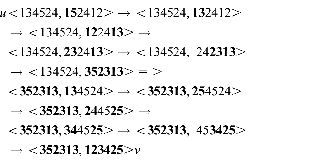
Because the worst-case time complexity of Algorithm 3 is 3n − 1, the worst-case time complexity of Algorithm 4 is 2(3n − 1)+1 = 6n − 1. Although Algorithm 4 is not optimal, the length of the path is less than or equal to the diameter in Theorem 3. For example, if the starting node u is <134524, 152412> and the destination node v is <352313, 123425> in OTIS–PSN₃, the routing path is as follows

\begin{matrix} u < 134524, 152412 > \to < 134524, 132412 > \\ \to < 134524, 122413 > \to \\ < 134524, 232413 > \to < 134524, 242313 > \\ \to < 134524, 352313 > = > \\ < 352313, 134524 > \to < 352313, 254524 > \\ \to < 352313, 244525 > \to \\ < 352313, 344525 > \to < 352313, 453425 > \\ \to < 352313, 123425 > v \end{matrix}

Broadcasting algorithm

Routing transfers a message from the node that has the message to another node. In contrast, broadcasting sends a message to every node in the network. Broadcasting is performed by successive calling to transmit a message and has several limitations: first, only two nodes participate in a call; second, a call is completed in a unit time; third, each node may take part in only one call in a unit time; and fourth, a call appears only between two neighboring nodes.²⁴ In one-to-all broadcasting, the originating node sends the message to all nodes, whereas in all-to-all broadcasting, each node has a different message, which it sends to all nodes. Here, we use one-to-all broadcasting. The one-port model allows a node to send a message to only one other node in a unit of time, whereas the multi-port model allows a node to send a message to multiple nodes. Here, we deal with the all-port model, which allows a message to be sent to all nodes in the same unit time.

The following is a brief overview of the broadcasting algorithm:

Stage 1. The message is sent to all nodes of the factor graph f to which belongs the node in which the message originated.

Stage 2. The message is transmitted to all the nodes that are connected to the nodes of f by o-edges. In each group, a single node receives the message.

Stage 3. In each group, Stage 1 is performed to simultaneously deliver the message to all nodes in the same group.

Next, to better understand the broadcasting algorithm, the broadcasting in OTIS–PSN₂ is examined. The node that initially had the message is called u = <g, p>|g = g₁ g₂ g₃ g₄, p = p₁p₂p₃p₄|g₁ g₂ =12, g₃ g₄ = 34, p₁p₂ = 23, p₃p₄ = 45. Here, xx ={12,13,14,15,23,24,25,34,35,45}, which are all the values that g₁g₂, g₃g₄, p₁p₂, and p₃p₄ can take. Thus, |xx| = 10. In Stage 1, a node u = <1234, 2345> transmits a message to a node set <1234, xx45> according to Algorithm 2. Here, the number of nodes with the message is 10. Node set <1234, xx45> then sends the message to node set <1234, 45xx>, connected by E₃. Here, the number of nodes with the message is 20. The node set <1234, 45xx> sends the message to another node set <1234, xxxx> according to Algorithm 2, and Stage 1 is terminated. Here, the number of nodes having the message is 100, and every node of factor <1234, xxxx>, to which u with the initial message belongs, has the message.

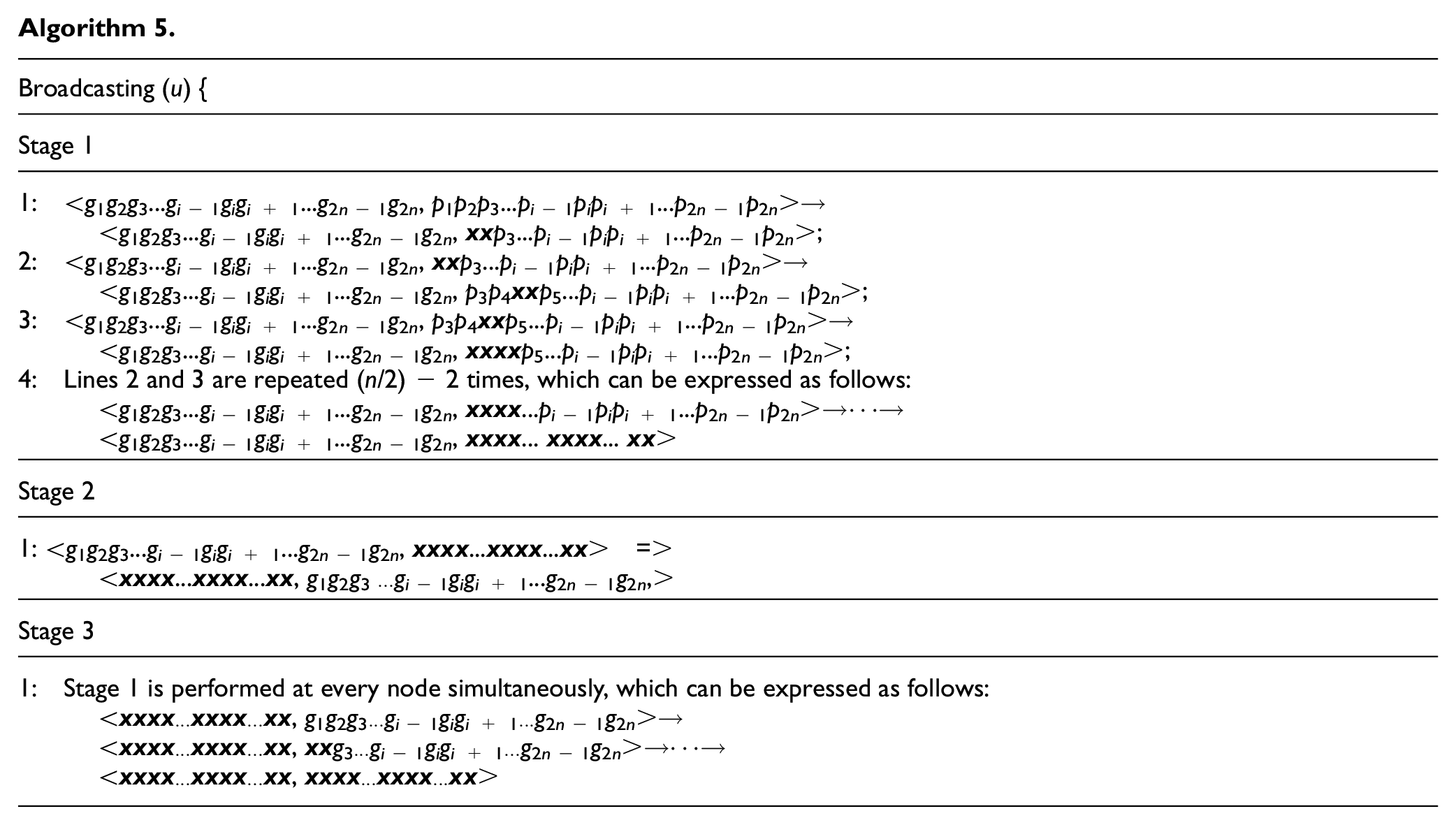
Stage 2 is simple. A node set <1234, xxxx> sends the message to node sets <xxxx, 1234> that are connected to each node by o-edges, and Stage 2 is terminated. Here, the number of nodes having the message is 200, and at least one node in every group has the message. In Stage 3, in each group, the node <xxxx, 1234>, which has the message from stage 1, sends the message simultaneously to all nodes <xxxx, xxxx> in the factor it belongs to. This can be generalized to create a broadcasting algorithm, as shown in Algorithm 5. The node that has the message first is called u = <g, p>|g = g₁ g₂g₃…g_i_− 1g_ig_i₊₁…g_2n − 1g_2n, p = p₁p₂p₃…p_i_− 1p_ip_i₊₁…p_2n − 1p_2n, and → refers to message transmission.

Algorithm 5.

Broadcasting (u) {
Stage 1
1: <g₁g₂g₃…g_i_− 1g_ig_i_+ 1…g_2n − 1g_2n, p₁p₂p₃…p_i_− 1p_ip_i_+ 1…p_2n − 1p_2n>→ <g₁g₂g₃…g_i_− 1g_ig_i_+ 1…g_2n − 1g_2n, xx p₃…p_i_− 1p_ip_i_+ 1…p_2n − 1p_2n>;2: <g₁g₂g₃…g_i_− 1g_ig_i_+ 1…g_2n − 1g_2n, xx p₃…p_i_− 1p_ip_i_+ 1…p_2n − 1p_2n>→ <g₁g₂g₃…g_i_− 1g_ig_i_+ 1…g_2n − 1g_2n, p₃p₄ xx p₅…p_i_− 1p_ip_i_+ 1…p_2n − 1p_2n>;3: <g₁g₂g₃…g_i_− 1g_ig_i_+ 1…g_2n − 1g_2n, p₃p₄ xx p₅…p_i_− 1p_ip_i_+ 1…p_2n − 1p_2n>→ <g₁g₂g₃…g_i_− 1g_ig_i_+ 1…g_2n − 1g_2n, xxxx p₅…p_i_− 1p_ip_i_+ 1…p_2n − 1p_2n>;4: Lines 2 and 3 are repeated (n/2) − 2 times, which can be expressed as follows: <g₁g₂g₃…g_i_− 1g_ig_i_+ 1…g_2n − 1g_2n, xxxx …p_i_− 1p_ip_i_+ 1…p_2n − 1p_2n>→⋯→ <g₁g₂g₃…g_i_− 1g_ig_i_+ 1…g_2n − 1g_2n, xxxx … xxxx … xx >
Stage 2
1: <g₁g₂g₃…g_i_− 1g_ig_i_+ 1…g_2n − 1g_2n, xxxx … xxxx … xx > => < xxxx … xxxx … xx , g₁g₂g_{3 ···}g_i_− 1g_ig_i_+ 1…g_2n − 1g_2n,>
Stage 3
1: Stage 1 is performed at every node simultaneously, which can be expressed as follows: < xxxx _··· xxxx _··· xx , g₁g₂g_3···g_i_− 1g_ig_i_+ 1···g_2n − 1g_2n>→ < xxxx _··· xxxx _··· xx , xx g_3···g_i_− 1g_ig_i_+ 1···g_2n − 1g_2n>→⋯→ < xxxx _··· xxxx _··· xx , xxxx _··· xxxx _··· xx >

Theorem 5

In OTIS–PSN_n, the time complexity for the one-to-all broadcasting algorithm of the all-port model is 3n − 7.

Proof

The time complexity of broadcasting Algorithm 2 is calculated. In Steps 1.1 and 1.3, the message is sent to 10 nodes of the Petersen graph to which it belongs, in only two times, according to broadcasting Algorithm 1. Step 1.2 is performed once. In Step 1.4, Steps 1.2 and 1.3 are repeated (n/2) − 2 times. The time complexity of Stage 1 is 2+(n/2 − 2) × (2+1) = 1.5n − 4. The time complexity of Stage 2 is 1. Because Stage 3 is the same as Stage 1, the total time complexity is 2(1.5n − 4)+1 = 3n − 7.□

Conclusion

In this article, we proposed an OTIS–PSN that has a small network cost and analyzed its basic topological properties. We then compared the network cost of previously reported OTIS networks with the proposed OTIS network (OTIS–PSN). OTIS–PSN_n has 10²ⁿ number of nodes, n+3 degree, and 6n − 1 diameter. If the number of nodes is N, the network cost of OTIS–PSN is $O ((lo g_{10} \sqrt[2]{N})^{2})$ . This is superior to the network cost $O ((lo g_{2} \sqrt[2]{N})^{2})$ of OTIS-hypercube, $O (\sqrt[4]{N})$ of OTIS-torus, and $O (\sqrt[2]{N})$ of the OTIS-swapped network. We also proposed a routing algorithm with a time complexity of 6n − 1, and a one-to-all broadcasting algorithm with a time complexity of 2n − 1. In OTIS networks, optical communication and electronic communication are used together for communication links. Further research should be conducted by applying the proposed algorithms to connected networks separately for electronic communication and optical communication, or particularly for optical communication.

Footnotes

Handling Editor: Dr Yanjiao Chen

Declaration of conflicting interests

The author(s) declared no potential conflicts of interest with respect to the research, authorship, and/or publication of this article.

Funding

The author(s) disclosed receipt of the following financial support for the research, authorship, and/or publication of this article: This work was supported by the National Research Foundation of Korea (NRF) grant funded by the Korean Government (MSIT) (no. 2020R1A2C1012363).

ORCID iD

Jung-hyun Seo

References

Seo

Lee

. Design and analysis of the rotational binary graph as an alternative to hypercube and torus. J Supercomput 2020; 76(9): 7161–7176.

Seo

Kim

Chang

, et al. The hierarchical Petersen network: a new interconnection network with fixed degree. J Supercomput 2018; 74(4): 1636–1654.

Marsden

Marchand

Harvey

, et al. Optical transpose interconnection system architectures. Optic Lett 1993; 18(13): 1083–1085.

Zane

Marchand

Paturi

, et al. Scalable network architectures using the optical transpose interconnection system. In: Proceedings of the third international conference on massively parallel processing using optical interconnections, Maui, HI, 27–29 October 1996, pp. 114–121. New York: IEEE.

Coudert

Ferreira

Muñoz

. Topologies for optical interconnection networks based on the optical transpose interconnection system. Applied Optics 2000; 39(17): 2965–2974.

Wang

Sahni

. Basic operations on the OTIS-mesh optoelectronic computer. IEEE Trans Parallel Distrib Syst 1998; 9(12): 1226–1236.

Lucas

Jana

. Parallel algorithms for finding polynomial roots on OTIS-torus. J Supercomput 2010; 54(2): 139–153.

Mahafzah

Jaradat

. The load balancing problem in OTIS-hypercube interconnection networks. J Supercomput 2008; 46(3): 276–297.

Awwad

. OTIS-star an attractive alternative network. In: Proceedings of the 4th WSEAS International Conference on Software Engineering, Parallel & Distributed Systems. World Scientific and Engineering Academy and Society (WSEAS), Stevens Point, WI, 13 February 2005. New York: ACM.

10.

Ahmad

. Topology-Based Analysis of OTIS (Swapped) Networks OKn and OPn. J Chem 2019; 2019: 1–11.

11.

Mahafzah

Sleit

Hamad

, et al. The OTIS hyper hexa-cell optoelectronic architecture. Computing 2010; 94(5): 411–432.

12.

Wei

Tao

. BSN-mesh and its basic parallel algorithms. Int J Grid Util Comput 2015; 6(3–4): 213–220.

13.

Gupta

Sarkar

. Biswapped–Torus network: a new efficient node-symmetrical optoelectronic network. Natl Acad Sci Lett 2021; 44(1): 27–31.

14.

Gupta

Sarkar

. BSN MOT: a fast and cost-efficient optoelectronic architecture. IETE Technical Review. Epub ahead of print 27 September 2020. DOI: 10.1080/02564602.2020.1823251.

15.

Gupta

Sarkar

. The recursive and symmetrical optoelectronic network architecture: biswapped network hyper hexa-cell. Arab J Sci Eng 2018; 43(12): 7635–7653.

16.

Parhami

Yeh

. Why network diameter is still important. In: Proceedings of international conference on communication in computing, Las Vegas, NV, 26–29 June 2000, pp. 271–274. New York: ACM.

17.

Ahmad

Hasni

Elahi

, et al. Polynomials of degree-based indices for swapped networks modeled by optical transpose interconnection system. IEEE Access 2020; 8: 214293–214299.

18.

Zahra

Ibrahim

Siddiqui

. On topological indices for swapped networks modeled by optical transpose interconnection system. IEEE Access 2020; 8: 200091–200099.

19.

Cancan

Ahmad

. Molecular descriptors of certain OTIS interconnection networks. Proyecciones 2020; 39(4): 769–786.

20.

Al-Adwan

Zaghloul

Mahafzah

, et al. Parallel quicksort algorithm on OTIS hyper hexa-cell optoelectronic architecture. J Parallel Distrib Comput 2010; 141: 61–73.

21.

Gupta

Singh

Bhati

. Efficient parallel algorithm for mapping LaGrange’s interpolation on OTIS and BSN hyper hexa-cell. In: 2020 international conference on emerging smart computing and informatics (ESCI), Pune, India, 12–14 March 2020. New York: IEEE.

22.

Memmi

Raillrd

. Some new results about the (d, k) graph problem. IEEE Trans Comput 1982; c-31(8): 784–791.

23.

Seo

Lee

. Design and analysis of the Petersen star interconnection network. Far East J Electron Commun 2017; 17(4): 719–732.

24.

Seo

Lee

. Link-disjoint broadcasting algorithm in wormhole-routed 3D Petersen-Torus networks. Int J Distrib Sens Netw 2013; 9(12): 1–7.

Petersen-star networks modeled by optical transpose interconnection system

Abstract

Keywords

Introduction

OTIS, Petersen graph, and PSN

OTIS

Petersen graph

PSN

OTIS–PSN

Definition

Topological properties of OTIS–PSN

Theorem 1

Proof

Theorem 2

Proof

Theorem 3

Proof

Theorem 4

Proof

Communication algorithm

Routing algorithm

Broadcasting algorithm

Theorem 5

Proof

Conclusion

Footnotes

Declaration of conflicting interests

Funding

ORCID iD

References